Linear root water uptake by vegetation

L

R

W

U

V

N. Ali

& S.W. Rees

1

Faculty of Civil Engineering, University Teknologi Malaysia, 81310; Tel. ++60 (7) 5531642 2

Cardiff School of Engineering, Queen’s Buildings, Cardiff CF24 3AA, UK; Tel. ++44(0)29 2087 4930

Corresponding Author : [email protected]

Abstract: The performance of a simple model with a linear root water extraction term that varies with time is presented in this paper. The research is based on the use of a one-dimensional form of Richard’s Equation for unsaturated moisture flow including a sink term. A numerical solution has been achieved via the finite element method for spatial discretisation along with a finite difference time-marching scheme. The model is assessed via a series of simulations of water uptake beneath uniform crop cover. A good correlation between the field data and simulated results has been achieved. This relatively straight forward approach is seemed more suitable for development and application to a range of geoengineering problems such as slope stability, shrinkage and heave prediction.

Keywords: Simulation, Suction, Tree Root, Unsaturated.

1.0 Introduction

The stability of soil slopes, naturally occurring or man-made, gives rise to significant problems in many countries. This is a problem that is exacerbated by climate change and increasingly intense rainfall events (Dehn et al., 2000; Turner, 2001). In many circumstances soil slopes will be populated by some form of vegetation ranging from grass cover to more established shrubs and trees. Repair maintenance and operation of railway and road embankments is a particular area where these problems are important (Ridley et al. 2004). Recent research indicates that progress is now being made to incorporate the influence of vegetation within the framework of slope stability analysis (Greenwood et al. 2004). Whereas, good progress is being made with regard to the contribution of roots to the overall shear strength, the direct influence of suction variations still requires further consideration.

In the UK, the shrinkage and swelling of clay soils, particularly when influenced by trees, is the single most common cause of foundation movements which may damage domestic buildings (BRE, 1999). In geoenvironmental engineering, one complementary technique that can be used to assist with the clean-up process is known as phytoremediation (Salt et al., 1995). This method exploits the soil/water interaction in the rhizosphere (root zone) to help remove contaminants from the soil mass. Therefore in this area also, an ability to predict the water uptake process will be useful.

There are many different root water uptake models described in the literature which classify these models into two categories which are the microscopic approaches and macroscopic approaches. In this paper, the macroscopic approach is used as this approach does not take into account the effect of individual root because of the difficulty in measuring the time-dependent geometry of the root system.

A considerable amount of research has been published in this area, starting with early contributions from Philip (1957) and Gardner (1964). Feddes et al. (1976) represented water uptake by roots by adding a volumetric sink term to the continuity equation for soil water flow. Further developments appeared in the literature shortly afterwards (see for example, Afshar and Marino (1978); Hoogland et al. (1981); Raats (1974); Landsberg and Fowkes (1978); Molz (1981); Rowse et al. (1978); Prasad (1988).

transpiration. An exponential root water uptake model was proposed by Li et al. (2001).

In the last few years, several findings have been published. For example, Homaee et al. (2002) used an extraction term in the simulation of salinity stress. Dardanelli et al. (2004) developed a simplified water-uptake model that uses generalizations from measured soil water content changes to predict root-water-uptake. Roose and Fowler (2004) provide a model which includes the simultaneous flow of water within the root network itself as well as within the soil mass. Braud et al. (2005) have provided a useful assessment of the water uptake that considered water stress compensation based on water stress reduction and an asymptotic root distribution function.

As a result, most of the models found in the literature are similar in approach, but these models use different root extraction functions. The model justified the use of these root extraction functions and each one of them operated successfully. Li et al. (2001, 2006) made a comparison of root water uptake models. Although they claim that an exponential model can produce more realistic behaviour compared to a linear model, they also demonstrate that only a 5 % difference in the cumulative water uptake occurred between these two approaches.

In view of the above, this paper develops a linear root water extraction term that varies with time based on the work of Prasad (1998). This simple approach lends itself to further development for application to wider range of geoenvironmental problems.

2.0 Unsaturated Moisture Flow Theory And Numerical Solution

The model employed is based on Richard’s equation (Richards, 1931) written in one-dimensional form and including a source/sink term:

(1)

Where K is the unsaturated hydraulic conductivity, t is the time, z is the

co-ordinates,

θ

This equation is written in terms of one unknown variable, the capillary potential, also frequently described as the negative pore-water pressure head.

The equation contains two soil properties; the specific moisture capacity

∂

θ

∂

ψ

S z K z

K z

t ∂ −

∂ +    

 

∂ ∂ ∂

∂ = ∂ ∂ ∂

∂ ψ ψ

ψ θ

and K. Both are non-linear functions of capillary potential (and therefore soil suction).

A solution of Equation 1 is obtained via a procedure of finite element spatial discretisation and a scheme of finite difference time-stepping. In particular, adopting a Galerkin weighted residual approach (Zienkiewicz and Taylor, 1989) yields:

(2)

In the work presented here, parabolic shape functions, and eight node isoparametric elements are employed. Using, Green’s formula and introducing boundary terms (Zienkiewicz and Taylor, 1989), lead to the final disctretised form: (3) Where : (4) (5) (6) (7) Ω ∂ ∫ ∂ ∂ ⋅ ∂ ∂ − Ω ∂ ∫       ∂ ∂ ∂ ∂ Ω Ω z N z K z K N z r r ψ ψ Ω ∂ ∫ ∂ ∂ ∂ ∂ − Ω ∂ ∫ ∂ ∂ + Ω Ω t N z K

N_{r r} ψ

ψ θ .

0

=

Ω

∂

∫

−

S

N

K s r

Ω ∂ ∫       ∂ ∂ = Ω ψ θ s rN N C

[

]

[ ]

∂

Ω

∫

=

S

N

S

+C J S

The time dependent nature of Equation 3 is dealt with via a mid-interval backward difference technique, yielding:

(8)

3.0 Development And Application Of A Sink Term

Equations describing one dimensional water uptake in a soil may be derived by assuming a linear variation of extraction rate with depth. It is assumed that for

potential transpiration conditions, Smax is given by,

(9)

Where Smax is the extraction rate, aj and –bj are the intercept and slope on the

jth day, respectively and z is the rooting depth. Let zrj is the maximum depth of

the root zone, the boundary condition at the bottom of the root zone (z = zrj) and

Smax equals to zero,

(10)

The total transpiration, Tj, across the root zone is then obtained by integrating

over the active depth,

(11)

Combining equations (10) and (11) give,

(12)

Integrating Equation (12), yields

(13)

0 2 1 2 1 1

2 1 1 2

1 _{+ + =}

    

  

∆ −

+ + + + +

+

+ n n

n n n

n n

S J

t C

K ψ ψ ψ

∫ ∂

= rj

Z

j S z

T

0 max

0

=

− _{j rj}

j b z

a

z

b

a

S

=

−

(

)

∫ − ∂

= rj

Z

j j

j a b z z

T

0

2

2

rj j rj j j

z b z a

At the bottom of root zone, from equation (10),

(14)

Substituting equation (14) into equation (13), yields

(15)

Substituting equation (15) into equation (14), then gives

(16)

Combining equations (9), (15) and (16), gives,

(17)

This can be re-arranged as,

(18)

Equation (18) is valid only under optimal soil moisture levels. When the moisture content is low, actual transpiration is lower than the potential value. A model proposed by Feddes et al. (1978) to describe the sink term for actual transpiration is represented by,

(19)

Where α is the prescribed function of the capillary potential. This function is

described in detail by Feddes et al. (1978) and will be discussed further. In Equation 19, when soil moisture is limiting,

(20)

rj j j b z

a =

2

2

rj j j

z T

b =

rj j j

z T

a = 2

z z

T z

T S

rj j rj

j

2 max

2 2

− =

    

  

− =

rj rj

j

z z z

T

S_max 2 1

( )

( )

S

ψ

α

ψ

(

)

  

  

− =

rj rj

j

z z z

T z

Prasad (1988) introduced this equation to represent one-dimensional water uptake model by plant roots. This equation is used in this paper.

4.0 Assessment Of The 1 -D Linear Model

An initial assessment of the model has been achieved by simulation of a series of test cases based on the experimental (and numerical) work of others. The results of this assessment are summarised below.

4.1 Case 1 - Linear Water-Uptake

The first case-study was based on the work of Mathur and Rao (1999). In this work, the soil water content was expressed a function of the pressure head using van Genuchten’s method (Genuchten, 1980):

(21)

Where

θ

θ

pressure head and, n and m are the empirical shape parameters. The parameters

used, for loamy soil, are shown in Table 1.

Table 1 : Basic soil properties Gottardi and Venutelli (1992)

Mathur and Rao (1999) used the water retention characteristic obtained from Equation 21 along with the pore size distribution model of Mualem (1976), to obtain:

(22)

r

θ

θ

(cm/h)

α l n m

0.0286 0.3658 22.54 0.0280 0.5 2.2390 0.553

(

)

( )

[

]

r s r

h

α θ θ θ

θ

+ − + =

1

(

)

(

)

2 1

1 1

+ −

+

  

 _{+ −}

=

l m n

n m

n

s

h h h

K K

1.0E+00 1.0E+01 1.0E+02 1.0E+03 1.0E+04 1.0E+05

0.01 0.05 0.09 0.13 0.17 0.21 0.25 0.29 0.33 0.37 0.41 Volumetric Water Content (%)

C a p ill a ry P o te n tia l ( c m )

Berino Loamy Sand

Where Ks is the saturated hydraulic conductivity and l is a soil specific

parameter. The water retention and hydraulic conductivity relationships are shown in Figures 1(a) and 1(b) respectively.

(a) Water Retention Curve (b) Hydraulic Conductivity

Figure 1: Material Properties for Berino Loamy Sand

The soil profile studied by Mathur and Rao (1999) was 100cm in depth. This was divided into 25 elements each of 4 cm height and 8 cm width. The moisture content initially was assumed to correspond to a capillary potential of -300 cm of water throughout the column. The boundary condition at the top was assumed to be a zero flux and the potential transpiration rate was assumed to be 0.025 cm/day. The maximum root length for the simulation was 13.66 cm and the period analysed covered four days. This problem has been re-analysed with the current model, to provide a basic verification of the sink term employed.

(a) 3 days (b) 4 days

Figure 2: Simulated Moisture Profiles at Day 3 and Day 4 1.0E-11 1.0E-10 1.0E-09 1.0E-08 1.0E-07 1.0E-06 1.0E-05 1.0E-04 1.0E-03 1.0E-02

0.01 0.11 0.21 0.31 0.41 Volumetric Water Content (%)

H y d ra u lic C o n d u c ti v it y ( c m /s )

Berino Loamy Sand

0 20 40 60 80 100 120

0.05257 0.05258 0.05259 0.0526 0.05261 0.05262 0.05263 Moisture Content D e p th ( c m )

Simulation 3 Day Mathur & Rao 3 Day

0 20 40 60 80 100 120

0.05256 0.05257 0.05258 0.05259 0.0526 0.05261 0.05262 0.05263 Moisture Content D e p th ( c m )

0 0.2 0.4 0.6 0.8 1

0 0.2 0.4 0.6 0.8 1 1.2 1.4 1.6 1.8

Capillary Potential (cm)

A

lp

h

a

The results for both the current simulation and those presented by Mathur and Rao (1999) for Day 3 and Day 4 are shown in Figure 2(a) and 2(b) respectively. The simulated results match well with the results from the previously published profile yielding some confidence in the implementation of the procedure.

4.2 Case 2 - Water Stress Function

The second case-study was based on the work of Feddes et al (1976). In their research, the finite different method was used to simulate sink term and was compared to the experimental result. A field experiment was performed by the Feddes (1971) at the groundwater-level experimental field at Geestmerambacht in the Netherlands, in which red cabbage was grown on heavy clay. Although the model did not predict the distribution of soil water content with depth in very accurate detail, the cumulative effect over the entire depth is properly simulated. The sink term which was used in their model is:

(23)

Where Epl is the actual transpiration (cm/s), Z is the rooting depth (cm) and

( )

ψ

α

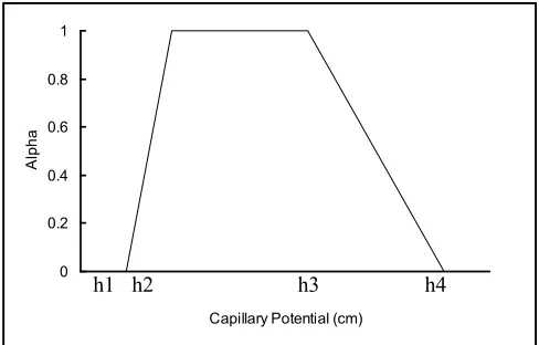
obtained in Figure 3. The root water uptake is zero when the soil is wetter than the anaerobiosis point, h1 as well as drier than the wilting point, h4 and is constant at its maximum value between h2 and h3. A linear variation of alpha, with capillary potential, is assumed when the latter is less than h2 or greater than h3.

h1 h2 h3 h4

Figure 3: General shape of the sink term as a function of the absolute value of the capillary potential, after Feddes et al (1978)

( )

( )

Z E

The water retention and hydraulic conductivity relationships for Case 2 are shown in Figures 4(a) and 4(b) respectively.

(a) Water Retention Curve (b) Hydraulic Conductivity

Figure 4: Material Properties for Heavy Clay

The soil profile was 100 cm in depth and was divided into 25 elements, each

of 4 cm height and 8 cm width. The moisture content initially was 0.5cm3/cm3

throughout the column and the boundary condition at the top was assumed to be a zero flux. The potential transpiration rate was assumed based on the average of 0.025 cm/hour. The depth of the effective root zone varied from about 25 cm at the beginning to about 70 cm at the end of the simulation which is 49 days. It is assumed that a uniform rate of root growth throughout the simulation which is 0.038 cm/hour.

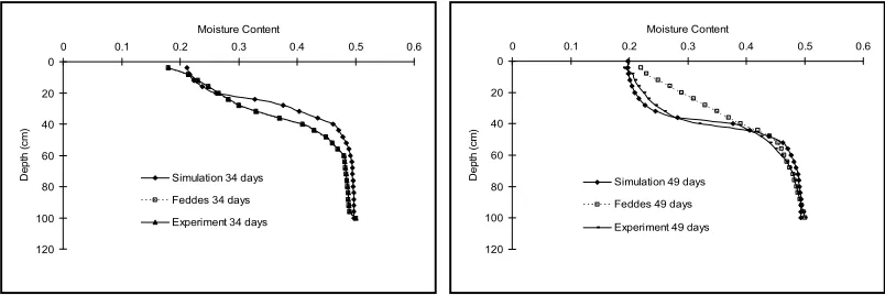
(a) 34 days (b) 49 days

Figure 5 : Simulated Moisture Profiles at 34 days and 49 days

1.0E+00 1.0E+01 1.0E+02 1.0E+03 1.0E+04 1.0E+05 1.0E+06 1.0E+07

0.01 0.16 0.31 0.46 0.61 Volumetric Water Content (%)

C a p ill a ry P o te n ti a l (c m

) Heavy Clay

1.0E-11 1.0E-10 1.0E-09 1.0E-08 1.0E-07 1.0E-06 1.0E-05 1.0E-04 1.0E-03 1.0E-02 1.0E-01

0.21 0.26 0.31 0.36 0.41 0.46 0.51 Volumetric Water Content (%)

H y d ra u lic C o n d u c ti v it y ( c m /s ) Heavy Clay 0 20 40 60 80 100 120

0 0.1 0.2 0.3 0.4 0.5 0.6 Moisture Content D e p th ( c m )

Simulation 34 days Feddes 34 days Experiment 34 days

0 20 40 60 80 100 120

0 0.1 0.2 0.3 0.4 0.5 0.6 Moisture Content D e p th ( c m )

Simulation 49 days Feddes 49 days

The results for the current simulation and those presented by Feddes et al (1976) in both finite difference simulation and experiment measured for 34 days and 49 days are shown in Figures 5(a) and 5(b) respectively. The simulated results match well with published profile at 34 days but slightly different with the finite difference result at 49 days. This difference may be occurring due to both simulations used different methods, different extraction functions and assumptions that have been made. However, the difference is small and acceptable which are 19 % and the simulation result profile looks close to the experiment measured profile.

4.3 Case 3 - Non-Uniform Root Model

The third case-study was based on the work of Gardner (1964). Gardner proposed a mathematical model to describe the water uptake by a non-uniform root system. The main thrust in this study was to determine the rooting distribution associated with each depth increment. The results of the model were validated using his experimental data on sorghum plant. The mathematical equation used by Gardner (1964) is:

(24)

Where q is the total rate of water uptake per unit cross sectional area by

summing from i=1 to i=n layer, B is a constant, h is the thickness for each n

layer,

δ

average matric suction in the soil, z is the distance from the soil surface to the

centre of the layer, k is the unsaturated conductivity of soil and L is the length of

roots in the unit volume of soil.

The water retention and hydraulic conductivity relationships for Pachappa Sandy Loamy are shown in Figures 6(a) and 6(b), respectively.

(

)

∑ − − =

=

n

i i i i i

L k z Bh

q

1

(a) Water Retention Curve (b) Hydraulic Conductivity

Figure 6: Material Properties for Pachappa Sandy Loamy

The soil profile was 200 cm in depth and was divided into 40 elements, which are concentrating at the soil surface. The linear distribution moisture content

initially used was from 0.3 cm3/cm3 to 0.4 cm3/cm3 at the depth of 100 cm from

the soil surface and the boundary condition at the top was assumed to be a zero flux. The potential transpiration rate is 2 cm/day. The maximum root length for the simulation was 100 cm and the period analysed covered four days. The maximum root length for the simulation was 100 cm and the period analysed covered four days.

(a) 2 days (b) 4 days

Figure 7: Simulated Moisture Profiles at 2 days and 4 days. 1.0E+00 1.0E+01 1.0E+02 1.0E+03 1.0E+04 1.0E+05 1.0E+06 1.0E+07

0.01 0.16 0.31 0.46 Volumetric Water Content (%)

C a p ill a ry P o te n ti a l (c m ) Pachappa Sandy Loamy 1.0E-13 1.0E-12 1.0E-11 1.0E-10 1.0E-09 1.0E-08 1.0E-07 1.0E-06 1.0E-05 1.0E-04 1.0E-03 1.0E-02 1.0E-01

0.01 0.11 0.21 0.31 0.41 0.51 Volumetric Water Content (%)

H y d ra u li c C o n d u c ti v it y ( c m /s ) Pachappa Sandy Loamy 0 20 40 60 80 100 120 140

0 0.1 0.2 0.3 0.4 0.5 Moisture Content D e p th ( c m )

Simulation 2 days Gardner 2 days Experiment 2 days

0 20 40 60 80 100 120 140

0 0.1 0.2 0.3 0.4 0.5 Moisture Content D e p th ( c m )

The results for the current simulation and those presented by Gardner (1964) in both calculation and experiment measured for 2 days and 4 days are shown in Figures 7(a) and 7(b), respectively. From both result, it is shown that the simulated results match well with published profile for both 2 days and 4 days.

5.0 Conclusions

This paper has presented an initial assessment of a 1-D linear water uptake model thought to be suitable for further development. Three case-studies have been presented for this purpose. The first case-study illustrated application of the linear water-uptake model to a simple hypothetical test problem. The new model produced results that were generally within 4 % compare to independently simulation results.

The second problem considered the significance of including a water-stress function for water-uptake modelling. The new model performed adequately for this type of problem. The final case study explored a problem involving a non-uniform root system. This problem served to illustrate the extent to which a simple linear approach could be used to model such a case. The linear model again performed adequately, but was, by definition, not capable of accurately representing a non-uniform extraction process. However, for some practical problems the cumulative water uptake predicted by a simple linear model may be adequate.

Overall, the new model has shown to be capable of producing results that are comparable with independently published results. The implementation of the water-uptake model and the associated sink term therefore appear to have been successfully undertaken.

Acknowledgement

Two anonymous reviewers are thanked for their helpful and constructive criticism.

Notations

( )

ψ

C

( )

ψ

K

Smax,

S

( ) ( )

ψ

,

S

ψ

,

z

T, Tj Potential Transpiration rate (cm/s)

zrj , zr Maximum rooting depth (cm)

( )

ψ

α

θ

r

θ

s

θ

ψ Capillary potential (cm)

References

Afshar, A., and Marino, M. A., "Model for simulating soil water content considering evaporation." Hydro, 37, 309-322, 1978.

Bouma, J., Jongmans, A. G., Stein, A., and G. Peek, "Characterising Spatially Variable Hydraulic Properteis of a Boulder Clay Deposit in the Netherlands." Geoderma, 45, p19-29, 1989.

Braud, I., Varado, N., and Olioso, A., "Comparison of root water uptake modules using either the surface energy balance or potential transpiration." Journal of Hydrology, 301, 267 – 286, 2005.

BRE, "Low-rise building foundations: the influence of trees in clay soils." A Building Research Establishment Publication, 1999.

Dardanelli, J. L., Ritchie, J. T., Calmon, M., Andriani, J. M., and Collino, D. J., "An empirical model for root water uptake." Field Crops Research, 87, 59 – 71, 2004.

Dehn, M., Burger, G., Buma, J. and Gasparetto, P., “Impact of Climate Change on Slope Stability using expanded downscaling.” Eng. Geology 55, p193-204, 2000.

Feddes, R.A. "Water, Heat and Crop Growth. " Agric. Univ. Wageningen, 71– 12, 184, 1971. Feddes, R. A., Kowalik, P. J., Malink, K. K., and Zaradny, H., "Simulation of field water uptake

by plants using a soil water dependent root extraction function." J. Hydro, 31, 13 – 26, 1976. Feddes, R. A., Kowalik, P. J., and Zaradny, H., "Simulation of field water use and crop yield."

Wageningen Center for Agriculture and Documentation, Wageningen, 189, 1978.

Gardner, W. R., "Relation of root distribution to water uptake and availability." Agronomy J., 56, 41 – 45, 1964.

Gardner, W. R., "Modelling water uptake by roots." Irrig. Sci., 12, 109 -114, 1991.

Genuchten, M. T. V. "A closed form equation for predicting the hydraulic conductivity of unsaturated soils." Soil Sci. Am. J., 44, 892 – 898, 1980.

Greenwood, J. R., Norris, J. E., and Wint, J., "Assessing the contribution of vegetation to slope stability." Geotechnical Engineering, 157(GE4), 199 -207, 2004.

Gottardi, G., and Venutelli, M., "Moving finite element model for one-dimensional infiltration in unsaturated soil." Water Resour. Res., 28, 3259 – 3267, 1992.

Homaee, M., Dirksen, C., and Feddes, R. A., "Simulation of root water uptake 1. Non uniform transient salinity using different macroscopic reduction functions." Agricultural Water Management, 57, 89 – 109, 2002.

Hoogland, J. C., Feddes, R. A., and Belmans, C., "Root water uptake model depending on soil water pressure head and maximum extraction rate." Acta Hort, 119, 276 -280, 1981.

Landsberg, J. J., and Fowkes, N. D., "Water movement through plant roots." Ann. Bot., 42, 493 – 508, 1978.

Li, K. Y., Jong, R. D., and Boisvert, J. B., "An exponential root water uptake model with water stress compensation." Journal of Hydrology, 252, 189 204, 2001.

Li, K. Y., Jong, R. D., Coe, M. T., and Ramankutty, N., "Root-water-uptake based upon a new water stress reduction and asymptotic root distribution function." Earth Interactions, 10, 2006.

Mathur, S., and Rao, S., "Modelling water uptake by plant roots." Journal of Irrigation and Drainage Engineering, 125(3), 159 – 165, 1999.

Mualem, Y. (1976). "A new model for predicting the hydraulic conductivity of unsaturated porous media." Water Resour. Res., 12, 513 - 522

Molz, F. J., "Models of water transport in the soil-plant system: a review." Water Resour. Res., 17(5), 1245 – 1260, 1981.

Philip, J. R., "The physical principles of water movement during the irrigation cycle." Proc. Int. congress on Irrig. Drain, 8, 124-154, 1957.

Prasad, R., "A linear root water uptake model." J. Hydrology, 99, 297 – 306, 1988.

Raats, P. A. C., "Steady flows of water and salt in uniform soil profiles with plant roots." Soil Sci. Am. Proc., 38, 717-722, 1974.

Rees, S. W., and Ali, N., "Seasonal water uptake near trees: a numerical and experiment study."

Geomechanics and Geoengineering., 1(2), 129 – 138, 2006.

Richards, L. A., "Capillary conduction of liquids in porous media." Physics, 1, 318 – 333, 1931. Ridley, A., McGinnity, B., and Vaughan, P., "Role of pore water pressure in embankment

stability". Geotechnical Engineering, 157, Issue GE4, p193-198, Paper 13714, 2004. Roose, T., and Fowler, A. C., "A model for water uptake by plant roots." Journal of Theoretical

Biology, 228, 155 171, 2004.

Rowse, H. R., Stone, D. A., and Gerwitz, A. "Simulation of the water distribution in soil." Plant Sci., 49, 534–550, 1978.

Salt, D. E., Blaylock, M., Kumar, N. P.B.A., Dushenkov, V. Ensley, B. D., Chet, I and Raskin, I., “Phytoremediation: A Novel Strategy for the Removal of Toxic Metals from the Environment Using Plants.” Bio/Technology 13, 468 – 474, 1995.

Turner, S., "Climate change blamed as landslip incidents treble." New Civil Engineer, 10 May, 2001, p8, 2001.

Warrick, A. W., Lomen, D. O., and Fard, A. A., "Linearized moisture flow with root extraction for three dimensional, steady conditions." Soil Sci. Am. J., 44, 911-914, 1980.