DSM-Based Methodology Development for Addressing Problems of High PV Penetrated Distribution System

PV Penetrated Distribution System. (Under the direction of Dr. Ning Lu).

Rooftop photovoltaic (PV) systems supply customer loads without the need of transporting electricity through long distance, making them an efficient distributed generation resource for supplying residential and small commercial loads. With the declination of the PV panel price and the installation cost, many areas such as Hawaii and California start to see large-scale deployment of residential and commercial roof-top PV systems [1].

However, because solar is a variable generation resource with intermittency and uncertainty in its power outputs, both the end users and the utilities would suffer some problems with the implementation of the PV panel. For end users, because there is a high possibility that the user consumption profile is not consistent with the PV power profile, the generated solar power cannot be efficiently utilized if no further measures such as installing appropriate energy storage (ES) or applying energy management programs could be implemented. For utilities, the intermittence of PV outputs may cause no or little operational issues as long as the solar penetration level is lower than 10% because power distribution systems are designed to handle large load variations. However, in areas where solar resources are abundant, policies support investment made towards PV installations, and environmental consciousness of residents are high, solar penetration levels are quickly reaching 20% or higher on some residential feeders. As a result, distribution grid operators start to observe overvoltage and reverse power flow at the point of connection and neighboring distribution networks [2-5].

DSM-Based Methodology Development for Addressing Problems of High PV Penetrated Distribution System

by Xiangqi Zhu

A Dissertation submitted to the Graduate Faculty of North Carolina State University

in partial fulfillment of the requirements for the degree of

Ph.D.

Electrical Engineering

Raleigh, North Carolina 2017

APPROVED BY:

_______________________________ _______________________________

Dr. Ning Lu Dr. David Lubkeman Committee Chair

_______________________________ _______________________________

DEDICATION

BIOGRAPHY

ACKNOWLEDGMENTS

My foremost and deepest gratitude goes to my advisor, Prof. Ning Lu, for her continual support, encouragement, and guidance. Prof. Lu is my role model, not only in academic study, but also in career and life. She showed me the way to be a good researcher and educator, and she always inspired me to pursue my dream. The invaluable advice she provided me on research, career development, presentation, technical writing, and many other aspects is a priceless fortune to me.

My great appreciation and thankfulness also goes to my committee members: Prof. David Lubkeman, Prof. Mo-Yuen Chow, and Prof. Yunan Liu, for their precious time and help. Their passion on research always motivated me to devote myself to my research and the exploration to the new areas.

I am also grateful for having many great lab mates in my life, I would like to express my sincere thanks to them: Jiahong Yan, Jiyu Wang, Xinda Ke，Jian Lu, Gonzague Henri, David Mulcahy, Weifeng Li, Fuhong Xie, and Ming Liang. All of the great memories with them are indispensable parts of my life.

TABLE OF CONTENTS

LIST OF TABLES ... vii

LIST OF FIGURES ... viii

CHAPTER 1 INTRODUCTION ... 1

1.1 HEMS Algorithm Development... 4

1.2 PV and ES Sizing Methodology and Tool Development ... 6

1.3 Cost-Benefit Study for Sizing PV and ES Systems ... 8

1.4 Voltage-Load Sensitivity Matrix (VLSM) Based Voltage Control ... 10

CHAPTER 2 DSM-BASED ENERGY STORAGE SIZING METHODOLOGY DEVELOPMENT ... 14

2.1 HEMS Algorithm Development... 14

2.1.1 Design Considerations of the HEMS Algorithm Development Toolbox ... 14

2.1.2 GUI Design and Modeling Approach ... 20

2.1.3 Case Studies ... 24

2.2 PV and ES Sizing Methodology and Tool Development ... 27

2.2.1 Data Preparation... 27

2.2.2 ESD Sizing Method ... 31

2.2.3 Simulation Results ... 41

2.2.4 Tool Interface Development ... 53

2.3 Cost-Benefit Study for Sizing PV and ES Systems ... 54

2.3.1 Modeling Methods ... 55

2.3.2 Setup of the Cost-Benefit Study ... 56

2.3.3 Cost-Benefit Study Results ... 60

CHAPTER 3 DSM-BASED VOLTAGE REGULATION METHODOLOGY DEVELOPMENT ... 67

3.1 A Hierarchical VLSM-Based DSM Strategy for Coordinative Voltage Control between T&D Systems ... 67

Nomenclature ... 67

3.1.1 VLSM and Price Functions ... 71

3.1.2 Optimization Control Strategy Modeling ... 75

3.1.3 Feeder Setup... 82

3.1.4 Feeder Analysis ... 88

LIST OF TABLES

Table 2. 1 Season Categorization for ESD Sizing Studies ... 31

Table 2. 2 TOU Price of Duke Energy ... 58

Table 2. 3 Price of PV Panel and ES ... 59

Table 2. 4 NPV of House1 ... 63

Table 2. 5 CA Rate Structure ... 66

Table 3. 1 Parameters for Price Functions ... 74

Table 3. 2 Main Steps of Load Disaggregation Process ... 86

Table 3. 3 VR Move Analysis... 91

Table 3. 4 Error Percentage for First Stage Control Case ... 92

Table 3. 5 Error Percentage for First Stage Control Case ... 94

Table 3. 6 Error Percentage for Second Stage Control Case ... 96

LIST OF FIGURES

Fig 1. 1 Dissertation Outline ... 3

Fig 1. 2 T&D interaction structure. ... 13

Fig. 2.1 The architecture of the FREEDM HEMS... 16

Fig. 2.2 The modeling of a virtual house ... 17

Fig. 2. 3 Modeling coupled load consumptions ... 18

Fig. 2. 4 Sample baseload profiles ... 19

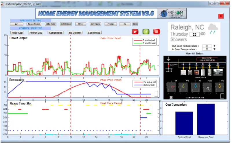
Fig. 2. 5 The main interface of the HEM GUI ... 21

Fig. 2. 6 Parameter setting interfaces for controllable loads ... 23

Fig. 2. 7 Calculation of probability of use ... 24

Fig. 2. 8 Total consumption of a house ... 24

Fig. 2. 9 Algorithm development flow ... 25

Fig. 2. 10 Result of price-cap control HEM algorithm ... 26

Fig. 2. 11 Result of solar-driven HEM algorithm ... 26

Fig. 2. 12 Examples of the load profile ... 27

Fig. 2. 13 Sample solar power output for PV panel of 6kW capacity ... 29

Fig. 2. 14 Sample appliance profiles generated using load models ... 30

Fig. 2. 15 Daily load duration curves for cold and warm months ... 31

Fig. 2. 16 Setup of the tri-level simulation ... 32

Fig. 2. 17 An ensemble of a summer day net loads for a house with a 4 kW rooftop PV ... 33

Fig. 2. 18 Control logic of the ESD for minimizing backfeeding energy ... 36

Fig. 2. 19 Daily operation sample of ESD ... 37

Fig. 2. 20 CDF of the daily backfeeding energy ... 38

Fig. 2. 21 Eneg for a range of PESDorEESD. ... 40

Fig. 2. 22 Q_ES and P_ESof different solar capacity ... 42

Fig. 2. 23 Sizing ESDs for different seasons ... 42

Fig. 2.24 Sizing ESDs for different homes ... 44

Fig. 2. 25 Sizing ESDs for aggregated homes ... 45

Fig. 2. 26 Sizing ESDs for 80% PV penetration level ... 46

Fig. 2. 27 Sizing ESDs for 100% PV penetration level ... 47

Fig. 2. 28 Size ESD for different PV penetration levels (80~100%) ... 47

Fig. 2. 29 Flow chart of controlling cooling loads for self-consumption of solar power ... 48

Fig. 2. 30 DSM impact on sizing ESDs at home-, transformer-, and community- levels ... 50

Fig. 2. 31 Backfeeding energy among different sizing methods ... 51

Fig. 2. 32 Results comparison of multiple years ... 52

Fig. 2. 33 Net present value of various ES sizes ... 53

Fig. 2. 34 Toolbox interface ... 54

Fig. 2. 35 Sample output of the load and PV models ... 56

Fig. 2. 36 On-Peak and Off-Peak period hours ... 59

Fig. 2. 37 Sample monthly savings ... 61

Fig. 2. 38 Sample yearly savings ... 61

Fig. 2. 39 Saving from PV (20 years) ... 62

Fig. 2. 40 Saving from PV (25 years) ... 62

Fig. 2. 42 Time schedule of CA rate ... 65

Fig. 2. 43 Bill saving comparison ... 66

Fig.3. 1 Price curves of controllable load (a) and PV (b) ... 75

Fig.3. 2 Probability density function for down j f ... 80

Fig.3. 3 Feeder topology of the IEEE 123-bus system ... 83

Fig.3. 4 Sample house load profiles ... 85

Fig.3. 5 Load disaggregation method ... 86

Fig.3. 6 Load profiles at the load bus on a distribution feeder ... 87

Fig.3. 7 Sample PV profiles ... 88

Fig.3. 8 Voltage profile comparison: with and without PV ... 89

Fig.3. 9 Profile boxplot comparison between without VR (a) and with VR (b) ... 90

Fig.3. 10 Voltage deviation comparison between without VR (a) and with VR (b) ... 90

Fig.3. 11 DR response at each node ... 91

Fig.3. 12 Voltage magnitude at each node ... 92

Fig.3. 13 DR response at each node ... 93

Fig.3. 14 Voltage magnitude at each node ... 93

Fig.3. 15 Required response amount of P and Q from transmission system ... 95

Fig.3. 16 Voltage profiles at bus 11 phase A ... 95

CHAPTER 1 INTRODUCTION

Rooftop photovoltaic (PV) systems supply customer loads without the need of transporting electricity through long distance, making them an efficient distributed generation resource for supplying residential and small commercial loads. With the declination of the PV panel price and the installation cost, many areas such as Hawaii and California start to see large-scale deployment of residential and commercial roof-top PV systems [1].

However, because solar is a variable generation resource with intermittency and uncertainty in its power outputs, both the end users and the utilities would suffer some problems with the implementation of the PV panel. For end users, because there is a high possibility that the user consumption profile is not consistent with the PV power profile, the generated solar power cannot be efficiently utilized if no further measures such as installing appropriate energy storage (ES) or applying energy management programs could be implemented. For utilities, the intermittence of PV outputs may cause no or little operational issues as long as the solar penetration level is lower than 10% because power distribution systems are designed to handle large load variations. However, in areas where solar resources are abundant, policies support investment made towards PV installations, and environmental consciousness of residents are high, solar penetration levels are quickly reaching 20% or higher on some residential feeders. As a result, distribution grid operators start to observe overvoltage and reverse power flow at the point of connection and neighboring distribution networks [2-5].

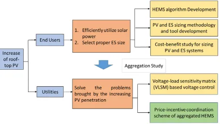
utilities from various aspects. In the first part of the dissertation, I focused my effort on developing residential PV and energy storage sizing methods considering demand-side management (DSM). Then, I studied the aggregated impact of high penetration of residential PV systems on distribution feeders operations. In the second part of the dissertation, I focused my effort on solving the voltage problems caused by PV integration. I developed a two-stage hierarchical control strategy for deploying demand response on distribution system, with the control objective of implementing demand response requirement from transmission system while regulating the voltage profiles at distribution system. This control strategy enables the co-optimization of demand response operation between the transmission and distribution systems. The Voltage-Load Sensitivity Matrix (VLSM) and the price functions for different demand response resources we developed have enabled us to consider the coordination among different demand response resources including both customer-owned and utility-owned devices. An outline for the research works I developed and will develop are shown in Fig.1.1. To size the residential PV and energy storage (ES) systems, the main consideration is to consume solar power for utility bill reduction. Therefore, the utility rates and the load characteristics including the controllability of loads are the predominant factors under consideration. My research focused on two aspects: design and develop home energy management algorithms to increase the controllability of home appliances and integrate cost-benefit analysis to help end users select PV and ES not only from the technical perspective but also from the economic perspective.

those changes, in the second part of my thesis I will conduct an aggregation study for thousands of homes on a few realistic feeder network model. To resolve the overvoltage and reverse power flow issues, I plan to develop two algorithms. The first algorithm is to use voltage-load sensitivity matrix (VLSM) based voltage control to select the right resources for regulating the voltage profile. The second algorithm will be a price-incentive coordination scheme for coordinating the demand response through price signals.

The state of art for each work will be introduced in the following part respectively, demonstrating what methodologies are in the literature and what approaches proposed in my dissertation.

1.1HEMS Algorithm Development

DSM programs are important resources for future power grid operation. DSM applications include improving energy efficiency, peak shaving and load shifting, load following and regulation, smoothing renewable generation outputs, and hedging high electricity prices [6-8]. In addition, DSM programs can greatly improve the flexibility, economics, and reliability of grid operation by coordinating distributed energy resources (DERs) such as electric vehicles, energy storage, distributed generations, and controllable load resources.

In the past, DSM resources are mainly large commercial and industrial loads [9]. The advancements in information technology, advanced sensor networks, data storage and processing capability, and communication make it possible to manage electricity consumption at end user level. Therefore, a major shift in DSM in recent years is focus on developing residential HEMS that allow residential customers to participate in energy efficiency and energy saving programs, as well as provide grid energy and ancillary services.

However, although the modeling of individual appliance can be relatively accurate, modeling residential household energy consumption remains a challenge. For example, how to accurately model the overall electricity consumption of a household under a wide range of consumption patterns and weather conditions? How to tune the devices and appliance models in the house model so that the modeled load profile matches the actual measurements?

There are three main technical challenges. The first one is to represent the correlation between different end use consumptions. For example, the modeling of electric water heater loads needs to be associated with the modeling of washers and dish washers. Otherwise the large amount of hot water when washing clothes or dishes cannot be reflected in the modeling process. The washer load needs to be connected with the dryer load because most of the dryer normally starts working minutes after the washer finishes its task. The second challenge is the modeling of non-controllable loads, which is highly random and has very little patterns to follow. The third challenge is to reproduce an actual load profile given a set of field measurements. Other considerations include the occupants’ behavioral patterns that dominate the energy consumptions of a household load. In general, a large amount of data is needed to quantify the resident’s behavioral patterns in a specific period of time as the behavior may change over time. As a result, unsupervised modeling normally can’t yield accurate results.

1.2PV and ES Sizing Methodology and Tool Development

Rapid power and voltage fluctuations along distribution feeders caused by behind-meter PVs have created serious operational issues such as overvoltage, reverse power flow, flickers, and equipment overloading [17-18]. ES can store energy for future use, smooth out large power fluctuations, and provide reactive power support to stabilize system voltage, making them one of the most effective technical solutions for the aforementioned operational issues. However, ESs are expensive. Comprehensive cost-benefit studies [19-22] have shown that the following strategies will make using ES more cost-effective: 1) providing multiple services to increase the utilization rate and revenue streams, 2) using DSM to reduce the size of ESDs, and 3) sharing ES among a group of users to reduce the amount of ES needed at the aggregated level.

Another technical challenge for the residential ES sizing study is the modeling of residential load consumptions. A typically approach is to use hourly average- or worst- case load profile derived from historical data for sizing ES. A major disadvantage of the approach is that it cannot account for the load pattern shift caused by behavioral changes of residential customers after the PV is installed. In addition, because both the PV generation and residential load consumptions are highly intermittent, considering a wider range of operation conditions is needed to size an energy storage system so that the performance of the ES will meet the requirements within a given risk margin.

power system applications published in literature. Therefore, we consider it is the main contribution of the work.

1.3Cost-Benefit Study for Sizing PV and ES Systems

If the capacity and the size of the storage component equipped for PV system are not well selected, the voltage variation and the back-feeding power may cause deterioration in grid operation. In addition, different utilities have different retail rate structures, it is critical to estimate whether or not for a specific residential or commercial load, installing PV system will be economic. Therefore, in this work, we present a series of cost-benefit study on residential PV and energy storage (ES) system installation options.

To mitigate the intermittence of the PV power output as well as increase the reliability of the power supply, installing a PV system with an energy storage system that coordinates with load management through HEMS is the best option for fully utilizing the potential of the residential roof-top PV systems [26-27]. Therefore, in this study we focus on sizing the capacity of the PV, PV-ES, and PV-ES-DR systems to satisfy the power supply requirements and study whether or not installing such PV systems is an economically viable decision.

the controllable loads can be shifted to periods when PV power is available. In addition, the rate structure also has a profound influence on the sizing of the PV and ES systems. If back-feeding power to the grid is not allowed (e.g. in Hawaii), it is then necessary to consider installing an energy storage system or invest on controllable loads so that PV power can be fully utilized. In both cases, detailed residential energy consumption needs to be used for sizing the needs for the PV and ES systems.

To facilitate the selection of PV and ES systems, we developed a method that can use a few customer inputs on their life styles to synthesize residential load profiles based on major appliance consumptions [30]. In this work, we present a cost-benefit study based on this method so that the synthesized residential loads can be used to simulate the impact of installing PV and energy storage systems of different capacity. The tariff we used in this study is the time-of-use (TOU) rate. Duke Energy time-of-use rate is used in major case studies, and PG&E time-of-use rate is added for comparison of bill saving brought by the PV-ES system under different rate structures. Four cases are designed and analyzed. Case 1 models residential loads with no PV and ES system installed and serves as the base case. Case 2 models the cases with only PV panels installed. Case 3 models the impact of installing an energy storage system together with the PV panels. In Case 4, we manage controllable loads to reduce the size of the storage system.

PV-ES system, comparing which option will be economically viable and has the best outcome in terms of money savings and performance.

1.4Voltage-Load Sensitivity Matrix (VLSM) Based Voltage Control

As mentioned before, advancements in solar power generation technologies significantly reduce the cost of roof-top PV systems in recent years [31]. The increasing environmental awareness among people together with subsidies and credits from the government and utilities are incentivizing more customers to install roof-top PV panels and consume greener power. Consequently, the installation capacities of roof-top PV systems are growing rapidly in recent years.

Ongoing studies have shown that high PV penetration causes voltage problems, such as rapid voltage variations and larger voltage ramps, in electric power distribution systems [17-18,32]. Those solar generation resources feed excess electricity from the distribution to the transmission systems, propagating the voltage problems to the transmission systems. More frequent and larger voltage fluctuations reduce the reliability and power quality of the power supply and require the voltage control devices to act more frequently to compensate for such fluctuations. Studies have shown that more voltage regulation devices are required in the distribution systems or the existing devices will need to act more often, causing significantly reduction of the lifetimes of those devices [33].

locations. Devices such as capacitor banks and mechanically switched shunt devices do not have many levels of control. Also, the frequent switching of those devices will significantly reduce their lifespan.

An alternative approach to resolve the voltage problems caused by high PV generation is to vary loads. When PV generation is high, we can increase electricity consumption; when clouds passing by, we can reduce the consumption. In recent years, although demand response (DR) programs have been extensively investigated for providing grid services for peak shaving, load shifting, and providing ancillary services[36-39], employing DR for voltage control has not yet been fully studied.

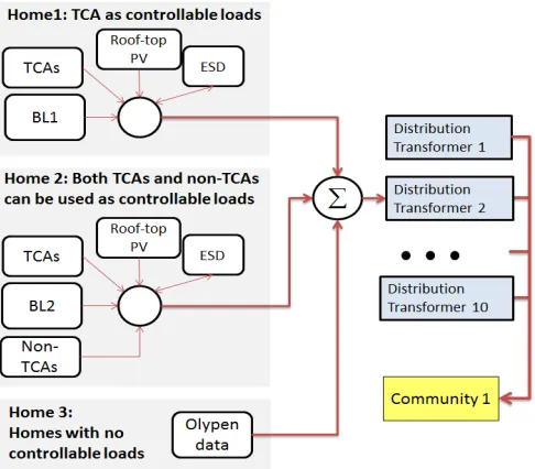
variability of PV has increasing influence on both T&D systems with high PV penetration. Therefore, in this work, we propose a hierarchical two-stage VLSM-based DR strategy for regulating the voltage at distribution feeders while fulfilling the transmission system DR requests. The setup is shown in Fig.1.2. To coordinate the voltage control between the transmission and distribution systems, at the beginning of each operation interval, controller at the transmission level will first perform optimal power flow to determine the optimal increase and decrease of the real and reactive power at each load node so that at the transmission level, the optimization objectives such as minimizing losses, cost, and voltage deviation could be satisfied. Then, the transmission system controller will issue to the distribution system controllers DR commands for them to determine how they will employ resources in their systems to provide the real and reactive power increase or decrease.

Fig 1. 2 T&D interaction structure.

CHAPTER 2 DSM-BASED ENERGY STORAGE SIZING METHODOLOGY DEVELOPMENT

This chapter introduces the methodologies developed for addressing the issues of end users in high PV penetration residential feeders. The work constructed on HEMS algorithm development, PV and ES sizing, and cost-benefit study for sizing PV and ES systems will be demonstrated correspondingly.

2.1HEMS Algorithm Development

This section is organized as follows. Sub-section 2.1.1 introduces the design considerations of the HEMS algorithm development toolbox. Sub-section 2.1.2 presents the GUI interface design and the modeling of the toolbox. Case studies are presented in sub-section 2.1.3. Conclusions and future research directions in this research area are summarized in sub-section 2.1.4.

2.1.1 Design Considerations of the HEMS Algorithm Development Toolbox

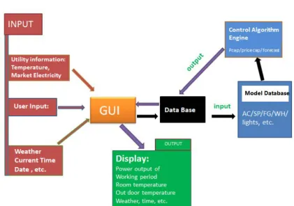
engines of the HEM system and algorithm selections can also be made through the GUI. Once an algorithm is selected, the user can call the appliance model parameters from the data base, run the algorithm, and generate simulation results, which are saved and sent back to the data base. Next, the GUI will display the results by reading data from the data base. This process allows the algorithm developers to develop and implement their algorithm independently while using the same model and operation conditions to compare the results generated through monitoring the results displayed by the GUI.

The standard setting of the smart house is a single-family home powered by a solar panel. The DERs include an energy storage device and electric vehicles. Each operation period is 24-hours and the simulation time step is 1-minute. There are three preloaded rate structures: flat rate, time-of-use, and critical-peak-price. Users also can define customized rate schemes through GUI inputs.

A. Design Consideration for the Graphical Interface

The considerations of the HEM GUI design are as follows [69]:

1) Provide a parameter setting interface for HEM controllable appliances and DERs. 2) Provide an input module that models the communication links with the other entities.

For example, the prices signal from the utilities, the weather information (e.g. outdoor temperatures and humidity) from the weather forecast providers, and utility control signals (peak-shaving, etc.) from the grid services aggregators.

3) Provide output displays that summarize performances for cost-benefit comparisons and status reports for monitoring device conditions.

Fig. 2.1 The architecture of the FREEDM HEMS

B. Design Consideration of the Models

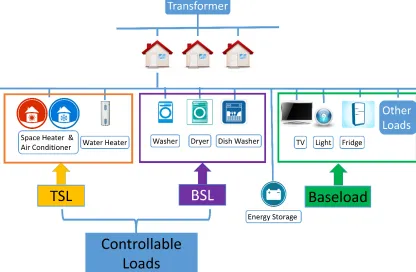
coupled so that the change of status of one appliance will trigger the change of status of all the other coupled devices. As shown in Fig. 2.3, all the appliances that use hot water are coupled. In addition, washer loads are also coupled with dryer loads. Dishwasher loads are coupled with cooking loads.

Fig. 2. 3 Modeling coupled load consumptions

The battery model developed in [43] is used in the toolbox. A salient feature of the battery model is that it includes a simplified lifetime estimation algorithm that allows the users to quantify the expected lifetime depreciation under different operation conditions.

As the modeling of distribution generation at the house level is mainly the modeling of rooftop PVs, we only included a PV model in the database. Because energy management is our main purpose, a simplified model that transforms the solar radiation data to the solar power outputs is used. However, we analyzed a few sets of PV data in North Carolina and developed a PV output database to represent different day types based on its probability of occurrence. This will allow the what-if scenarios to reflect the performance from a probabilistic-based approach.

0

5

10

15

20

25

0

5

10

15

Time of the day (min)

C

ons

um

pt

ion (

k

W

)

P

house

P

washer

P

P

P

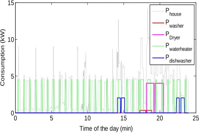
The main technical challenge in developing a base-load database is the separation of major controllable appliance consumptions from the must-run house appliance loads. Load desegregation methods are applied on measurement data of 50 houses collected in 2006-2007. Then, the normalized realistic load profiles of the 50 houses are used to establish the base load pool by a number of clustering methods (e.g. baseline power and energy consumptions and different occupancy patterns). Fig. 2.4 shows an examples of the baseload profiles. There are two types of baseloads. Baseload 1 (BL1) is the baseload without TSLs and Baseload 2 (BL2) is the baseload without both BSLs and TSLs. This allows the algorithm developers to superimpose the controllable loads on the baseload to form different type of end use patterns. The baseloads are different for each season and covers high, medium, and light electricity consumption patterns.

2.1.2 GUI Design and Modeling Approach

In this section, we briefly describe how to seamlessly integrate the models into a flexible modeling platform for algorithm development by meeting the modeling considerations presented in Section II.

A.Graphical Interface Design

Fig. 2. 5 The main interface of the HEM GUI

B.Modeling Behavior Sensitive Loads

BSLs are modeled using randomized arrivals and consumer designated time slots. Two approaches are used to model BSLs: consumer designated time slots and randomized arrivals. The modeling principles of the two methods are described as

P t_i( )=P_iratedS t( ) (2.1)

P t_i( )=P_iratedp t_i( ) (2.2)

where ( )P ti is the power consumption of load iat time t; S t( )is the on (1)/off (0) status of

the load;Piratedis the rated power of load i, and p ti( ) is the probability of use of load iat time

For method of consumer designated time slots, as shown in (1), the power consumption of load i at designated time t (see Fig.2.6) when this load is on, is defined as its rated power. For method of randomized arrivals, the power consumption of load i at time t is calculated by multiplying its rated power by the probability it will be on at this time slot. The method of randomized arrivals is usually used in large scale simulation which involves lots of homes. The probability of use is calculated from the data base which is composed of field measured data of the appliances in the houses.

The probability of use of load iat time tis calculated by

1/ ( ) ( ) N i i rated i P t p t P

= (2.3)

1/ ( )

( ) N N i i P t P t N

= (2.4)

where 1/N( )

i

P t is the average consumption of load i at time tin one house and N( )

i

P t is the

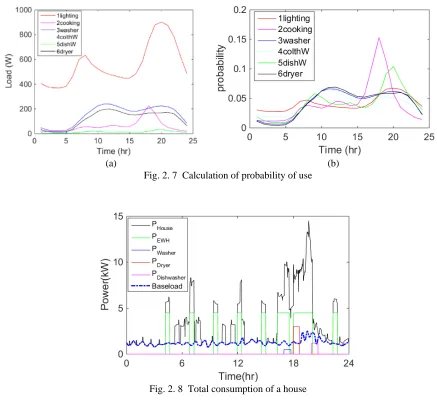
total consumption of all the load i at time tof a community with N houses. Fig. 7 demonstrates

the calculation of the probability of use of BSLs. Fig. 2.7 (a) shows the P_i1/N( )t of a sample day, and Fig. 7 (b) shows the corresponding probability of use calculated from Fig. 2.7 (a).

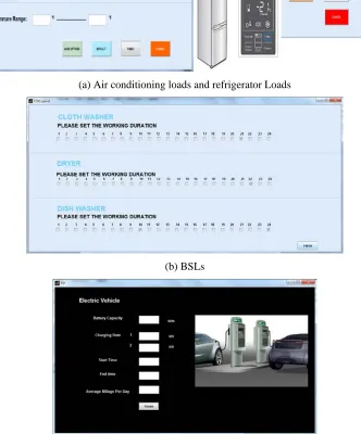
(a) Air conditioning loads and refrigerator Loads

(b) BSLs

(c) Electric vehicles

(a) (b) Fig. 2. 7 Calculation of probability of use

Fig. 2. 8 Total consumption of a house

2.1.3 Case Studies

incorporating the ES and PV model, the house can be operated off-grid and simulate the HEM in Microgrid operation modes.

Fig. 2. 9 Algorithm development flow

Several HEM algorithms have been developed on this modeling platform. Two examples are shown in Fig. 10 and 11 to demonstrate the effectiveness of the toolbox. As shown in Fig. 10, a price-cap control HEM algorithm for reducing the electricity payment is modeled and compared with the no-HEM-control case. The TSLs and BSLs will be deployed to reduce the electricity consumption according to the priority list determined by the customer. The red circled areas represent decreased consumption during high price intervals.

Because the same set of appliance models are used, the performance of different algorithms can be compared on a fair basis. In addition, students are invited as guests for testing the performance of the algorithms. The data are stored in the database so that the customer behaviors can be analyzed.

Fig. 2. 10 Result of price-cap control HEM algorithm

2.2PV and ES Sizing Methodology and Tool Development

This section is organized as follows. Sub-section 2.2.1 describes the data used in the study. Sub-section 2.2.2 introduces the energy storage sizing considerations and methods. The simulation results are discussed in sub-section 2.2.3. Sub-section 2.2.4 summarizes the conclusion.

2.2.1 Data Preparation

A. Load Data Preparation

The residential load data used in the work is collected by Pacific Northwest National Laboratory at Olympia Peninsula (the Olypen data), WA in the GridWise demonstration project [44]. Energy consumptions of 50 residential homes were measured at 15-minute resolution for a year (April, 2006 - March, 2007), so there are 96 data points for a 24-hour period. At Olympia Peninsula, air conditioners are operated only occasionally in summer because of the mild weather in the area, thus the cooling loads can be filtered out by clustering load profiles into “a/c on” and “a/c off” days. Then, disaggregation methods [45-46] can be used to obtain the Baseload 1 (BL1) profiles that contains temperature-insensitive loads, as shown in Fig. 1(a).

(a) (b)

Similar clustering methods also allow us to obtain Baseload 2 (BL2) profiles that exclude infrequently-used, controllable residential loads (e.g. washers, dryers, and dishwashers), as shown in Fig. 2. 12(a) [47]. The BL2 loads are mainly uncontrollable loads such as cooking, lighting, and refrigerating loads. Thus, baseload profiles randomly selected from the BL1 and BL2 databases, together with the controllable load profiles created by load models, can be used to model residential household loads. This hybrid load profile synthesis process allows us to preserve the correlation between the outdoor temperature and the cooling and heating load consumptions. In addition, the method makes it possible for us to model the control of load-side resources for reducing the size of the ESD. This process is a critical step for producing residential load profiles to generate the net load ensembles and is one of the main contributions of this study.

In this study, we assume that a distribution transformer supplies up to 5 residential homes and a community supplies up to 50 homes. Examples of the aggregated load profiles at the transformer- and community- levels are shown in Fig.2.12 (b).

B. Solar Data Preparation

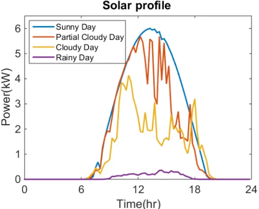
The solar radiation data is converted to PV generation profiles with the consideration of conversion efficiency as 20% [49]. A solar output database including four basic solar profiles (sunny, partially cloudy, cloudy, and rainy) was created, as shown in Fig. 2.13.

Fig. 2. 13 Sample solar power output for PV panel of 6kW capacity

C. Controllable Appliances Modeling

D. Seasonal Impact on Energy Storage Size Selection

Fig. 2.15 shows daily average load duration curves for a residential home and the average daily high and low temperatures of each month. The Olypen load is winter-peaking because electric space heaters are used. In summer months, the average daily high temperature is about 25°C, so the cooling load is low. Because load consumption patterns are very different in the summer and winter seasons, we divided the yearly data into two seasons: cold and warm, as shown in Table 2.1. This allows us to address the difference in energy storage size selection caused by seasonal load variations [66].

Fig. 2. 15 Daily load duration curves for cold and warm months

Table 2. 1 Season Categorization for ESD Sizing Studies

Cold season November, December, January, February,

March

Warm season April, May, June, July, August,

September, October

2.2.2 ESD Sizing Method

The ESD sizing procedure and methodologies are presented in the following subsections.

A. Setup of the Tri-level Simulation

TCA models. For homes using both TCAs and non-TCAs as controllable loads, baseload profiles from the BL2 database are used.

At home-level, the PV installed capacity ranges from 1kW to 6kW. ESDs within a community can be shared for storing excess solar generation to decrease reverse power flow and smooth power variations

Fig. 2. 16 Setup of the tri-level simulation

B. Energy Storage Sizing Method

There are three key steps in the energy storage sizing method as illustrated below. Step 1. Generate the ensemble of the net load profiles

The first step of the sizing process is the calculation of the ensemble of the home net load profiles using a shuffling algorithm. LetPSolar be the power output of the rooftop PV and PLoad

be the total household load consumption, the net loadPnet, can be calculated as

( , ) ( , ) ( , )

1, 2,..., 152 213

1, 2,..., 96

net Load Solar

Cold Warm

days days days data data

P i j P i j P i j

i N N N

j N N

= −

= = =

= =

where i is the th

i day, and jis the jthdata point. In our residential load database, there are 152 days in the cold season and 213 days in the warm season. Hence, Cold

days

N =152 and Warm days

N

=213. Ndata represents the data number in a day. The consumption is metered every 15-minute,

hence Ndata is equal to 96.

The shuffling algorithm works as follows.Take warm season as an example,for the ith day

load profile, replace the solar radiation data of the ithday with that of the other 212 days to

obtain an ensemble of net load profiles for the ith day. This process can be represented by

Load

Load

Load

Load

( ,1: ,1) ( ,1: ) (1,1: )

( ,1: , 2) ( ,1: ) (2,1: )

( ,1: ) ( ,1: )

( ,1: , )

( ,1: ) ( ,1: )

( ,1: , )

net Solar net Solar Solar net Solar days net days

P i j P i j P j

P i j P i j P j

P k j P i j

P i j k

P N j

P i j P i j N

= −       (2.6)

k=1, 2,...,N_days

The ensemble of a summer day net loads is shown in Fig. 2.17.

Fig. 2. 17 An ensemble of a summer day net loads for a house with a 4 kW rooftop PV

0 5 10 15 20 25

-5 0 5 10 15

Time of the day (hour)

P net

(k

W

)

To obtain the ensemble M of the net load profiles for the whole season, repeat this process for all load profiles in the seasonal database (e.g.NdaysCold =152,NWarmdays =213):

296

(1,1: ,1) ...

(1,1) ... (1, 96) (1,1: , )

(2,1) (2, 96)

( ,1: ,1) ...

( ,1: , )

( ,1: ,1) ₍

...

( ,1: , )

days net

net days

net

net days

net days _days

net days days _N

M

P j

M M

P j N

M M

P i j

P i j N

P N j _{M N N}

P N j N

× =                   =             _×             

,1) ... ( , 96)

days M Ndays Ndays

                       ×    (2.7)

For instance, the ensemble matrixMfor the warm season will include 213 213× net load profiles. This process is highly scalable. When more load and solar radiation data becomes available, Ndayscan be increased to obtain more solar-load combinations. Shuffling the solar

radiation data of the entire season against a load profile might result in unrealistic cases. However, the more measurements we have in the database, the closer the obtained net load profiles reflect the actual statistics because the unrealistic cases will become outliers that have little impact on the final result.

Step 2. Perform capacity-iteration

Although home-owned ESDs can be used for a variety of purposes, one of the main reasons for the consumer to own an ESD is to self-consume the solar power. Therefore, in this study,

the ESD is controlled to minimize the backfeeding energy. Let P_ESD( )t represent the power

negative when charging and positive when discharging. Then, the power difference at timet, ( )

P t

∆ can be calculated as

∆P t( )=P_load( )t −P_solar( )t −P_ESD( )t (2.8)

DefineP_neg( )t as the power backfed to the main grid and calculate P_neg( )t as

( ) 0, ( ) 0

( ) ( )

neg neg

if P t P t

else P t P t

∆ ≥ =

= −∆ (2.9)

Then, the objective of sizing home-owned ESD is to minimize the total backfeeding energy

neg E :

1

min ( )

T neg neg

t

E P t

=

=

∑

where Enegis the total backfeeding energy and T is the total time. Let

Max ESD

E and Min ESD

E be the upper

and lower charging limits of the ESD and t ESD

E be the energy level of ESD at time t. The above optimization problem can be solved by a straight forward control strategy shown in Fig. 7. The ESD will be charged whenever P_nett <0 &E_ESDt <E_ESDMax , and discharged whenever

0 &

t t Min

net ESD ESD

P > E >E . Note that in our study, Ref

net

Fig. 2. 18 Control logic of the ESD for minimizing backfeeding energy

An example of the daily operation of an ESD is shown in Fig. 2.19. For a given combination of PESD andEESD, we run the algorithm to calculateEnegfor all the net load profiles in M. This will

result in 213 213× and152 152× sets of Enegvalues in the warm and cold seasons, respectively.

Fig. 2. 19 Daily operation sample of ESD

The CDF curve of the backfeeding energy in the cold season for a 3kW/3kWh ESD is shown in Fig. 2.20(a) and is compared with the CDF curve of the No-ESD case. LetEESD equal to 1kWh

andPESD increase from 1kW to 5kW. We calculate the CDFs of the five cases and plot them in

Fig. 2.20(b). The zoom-in plot in Fig. 2.20(c) at the 80% quantile shows that increasing the power rating from 1kW to 5kW while maintaining the energy capacity at 1kWh can only reduce Eneg by 0.4 kWh. This shows that the energy capacity of the ESD is the key limiting

factor.

5 10 15 20

-5 0 5 10 15 P net (k W )

5 10 15 20

-5 0 5 P (k W ) _P ESD P neg

5 10 15 20

0 5

Time of the day (hour)

(a)

(b) (c)

Fig. 2. 20 CDF of the daily backfeeding energy

Let Target neg

E represents the user defined backfeeding energy constraints. To find the smallest

ESD

P and EESDthat can meet the constraints, if Enegmeets the targeted values of

Target neg

E , we will

reduce the PESD or EESDby

Band ESD P

∆ or ∆EESDBand, respectively, until the

Target neg

P and Target neg

E cannot be met; if

neg

E cannot meet the targeted values of Target neg

E , we will increase thePESDor EESDuntil the

Target neg

P and

Target neg

The cost difference,∆C, between self-consuming Target neg

E and selling Target neg

E to the grid, can be

calculated as

Target

neg ( buying selling)

C E p p

∆ = × − (2.11)

wherepbuyingis the price at which utilities buy extra solar power from the homeowners, and

selling

p is the price for selling grid power to users. This allows the home-owner to determine

Target neg

E based on electricity prices. Another way of determining Target neg

E is the utility requirement at

the point of coupling. In this study, our focus is to develop the sizing procedure and methodologies for comparing different sizing options based on the net load ensembles. Therefore, we assume that the value of a desired Target

neg

E has been computed and is a known input

of the sizing problem.

Step 3: Generate the compressed, composite CDF curve and use the Equal Probability Line

method to select the optimal ESD size

By compressing the x-axis of Fig. 2.20 into a 0-1 block, we can put the CDF plots of different battery size options side-by-side in one figure to create a compressed, composite CDF (CC-CDF) plot for comparing the different options. As shown in Fig. 2.21, one CC-CDF plot

consists of 25 CDFs that represent fiveEESD size options (1, 2, 3, 4, and 5kWh) and five PESD

y-axis of the intersection between the EPL and the CDF curves, the user can quickly find an ESD size for his home to meet a the daily backfeeding energy limit 80% of time. Assume that a customer wants to install a battery for a 6-kW PV system and he wants the backfeeding power to the grid below 1.5 kWh 80% of time. As shown in Fig. 2.21, as long as the battery energy capacity is above 2kWh, the customer’s requirement can be satisfied. Once the battery energy rating is above 3kWh and power rating is above 2kW, the marginal reduction of backfeeding energy by increasing the battery energy and power sizes are diminishing, so the customer may want to choose at most a 3 kWh/2kW battery. If the battery cost is also known, how much it costs to reduce backfeeding energy for any given PV capacity could also be calculated.

Fig. 2. 21 Eneg for a range of PESDorEESD.

evaluations with multiple optimization variables associated with monotonically increase or decrease continuous or discontinuous functions. Therefore, the development of this graphical method is considered to be one of the main contributions of this work.

2.2.3 Simulation Results

In this section, simulation results for sizing home-owned ESDs, transformer-ESDs, and community-owned ESDs are presented. FiveEESD options (1, 2, 3, 4, and 5kWh) and five rated

power options (1, 2, 3, 4, and 5kW) are considered for six installed PV capacities (1, 2, 3, 4, 5, and 6kW). Two different load patterns (winter and summer) are compared to assess the necessity of sizing ESDs for different seasons. The capabilities of using DSM to reduce the size of the ESD are also assessed. For all the cases, results are produced using the capacity-iteration method and analyzed by projecting the 80% EPLs on the CC-CDF curves as introduced in Section III.

A. Size the ESD Considering the Seasonal Load Pattern Shifts

The CC-CDF curves for the cold month loads are shown in Fig. 2.22. The 80% EPLs for installing a 4, 5, and 6-kW PV system are plotted for selecting the power and energy capacities of the energy storage system based on the daily backfeeding energy limit, Target

neg

E . The figure

shows that if the PV capacity is less than 5kW and Target neg

E is 1.5 kWh, there is no need for using

an ESD. If the PV capacity is 6 kW, a 1kW/2kWh ESD may meet the Target neg

E 80% of the time.

Fig. 2. 22 Q_ES and P_ESof different solar capacity

The CC-CDF curves of the summer months are shown in Fig. 2.23 by repeating the above analysis for the summer months. To better demonstrate the seasonal difference, as mentioned in Section 2.2.1, a set of solar radiation data collected in the same area where the load data was collected is used to do the same analysis.

Fig. 2. 23 Sizing ESDs for different seasons

Note that most houses in Olympic Peninsula have very low air conditioning loads because of the mild weather in that area. Therefore, in the summer months, the self-consumption capability of a household is very limited. As a result, there is a greater need for storing energy to meet the same Target

neg

seasonal needs of energy storage can be very different. For example, in Southern cities, winter loads are low and summer loads are high, so the capability of self-consumption are higher in summer. Thus, ESD renting programs for meeting the different seasonal needs between summer and winter peaking regions may become an economic solution.

B. Size the ESD for Aggregated Residential Loads at the Transformer- and Community- Levels

The ESD sizing curves for 4 homes with 6-kW PV systems in the cold months are shown in Fig. 2.24. The CDF of the daily backfeeding energy of each home can be very different because each home has its unique consumption pattern and load characteristics. For example, a gas-heating residence has significantly lower energy consumptions than an electric-gas-heating one. When multiple homes share an ESD, the load diversity tends to increase the self-consumption capacity and reduce the ESD size.

Fig. 2.25 shows the results of sizing ESD for 2~3 homes. As expected, backfeeding energy decreases significantly for the same total ESD capacity. For instance, if home 2 and home 3 each has a 1kWh/1kW ESD, Enegcan reach approximately 14kWh. However, if these two

Fig. 2. 25 Sizing ESDs for aggregated homes

Define the PV penetration level of the community as the percentage of the homes in the community that have PV installed. The CC-CDF of a community with 33 homes using their winter net load ensembles is calculated. For each home with PV installed, the installed capacity is assumed to be 6kW. As shown in Fig. 2.26, if the penetration level is less than 80%, there is no need to install an ESD using the following criteria: “ Target

neg

E is less than 1kWh 80% of

Fig. 2. 26 Sizing ESDs for 80% PV penetration level

However, if the penetration reaches 100% (see Fig. 2.27) as all the 33 homes have a 6-kW PV system installed, Eneg can increase significantly. If the capacity of the community ESD is

still 1kWh/1kW, Eneg can be controlled to be less than 15kWh 80% of time. Fig. 2.28 (a) shows

the performances of different ESD capacity options when the PV penetration level increases from 80% to 100%. The plot also shows the expected improvement per capacity increase.

Set Target neg

E of a community at 8kWh. Assume each house in the community has a 6kW PV

Fig. 2. 27 Sizing ESDs for 100% PV penetration level

(a) (b)

Fig. 2. 28 Size ESD for different PV penetration levels (80~100%)

C. Sizing ESDs Considering Demand-side Management

(AC) unit is controlled to assist the self-consumption of the PV power. The AC will operate within a temperature bandTlow,Thigh. The middle of the band is the AC set pointTset. At every

time step, Psolar (t) and Pload (t)will be checked, if Psolar (t)>Pload (t), then the AC status and

room temperature will be checked successively. If AC is “off” and room temperature is higher than Tset, AC will be turned on to cool the room.

Psolar(t)>Pload(t)?

AC is on?

Yes

Troom > Tset

No

Turn on AC No action

Yes

No No

Yes

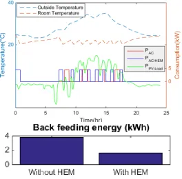
Fig. 2. 29 Flow chart of controlling cooling loads for self-consumption of solar power

The simulation results at the home-, transformer-, and community- levels are shown in Fig. 2.30.

1) Home-level study

Fig. 2.30(a) shows the results of sizing the ESD with- and without- DSM at the home level. Applying DSM will decrease the size of the ESD significantly. For instance, if the ESD is

2) Transformer-level study

The simulation results at the transformer level are shown in Fig. 2.30(b). The percentage of

neg E

reduction is around 34% after using DSM. The size of the ESD is 3kW/1kWh to maintain

the

Target neg

E

below 10kWh without DSM. With DSM, the size of the ESD is reduced to 1kW/1kWh, representing a 67% reduction.

3) Community-level study

To further investigate the aggregation impact of using DSM for helping reducing the size of community ESD, aggregated loads of 33 homes (each home has a 3kW roof PV system) are

(a) (b)

(c)

Fig. 2. 30 DSM impact on sizing ESDs at home-, transformer-, and community- levels

D. Comparison with Other Sizing Methods

In the literature, many sizing methods use the worst case scenarios or the average case scenarios for sizing ESDs. To compare with the results obtained by those sizing methods, Eneg

the net load in a sunny, average load day. If a 5-kW PV and a 3-kW ESD are selected, we can compare the energy capacities of the ESD selected by different sizing methods.

Assume that Target neg

E is 6kWh, the proposed sizing methodology suggests that the user can

use a 3kW/1kWh ESD for the warm months and no ESD is needed in the cold months. The average case method suggests that no ESD is needed and the worst case method indicates that a 3kW/3kWh ESD is needed for an entire year. The comparison shows that the average case tends to underestimate the ESD needs and the worst case tends to overestimate the ESD needs depending on how the worst case is constructed.

Fig. 2. 31 Backfeeding energy among different sizing methods

E. Comparison using Data from Multiple Years

simulation results show that except for a few years, the results obtained using the proposed method are consistent. If more data are available, the upper and lower boundaries of the sizing curve can be obtained to further enhance the results.

Fig. 2. 32 Results comparison of multiple years

F. Cost-benefit Analysis under TOU Tariff

(a)

(b)

Fig. 2. 33 Net present value of various ES sizes

2.2.4 Tool Interface Development

can either optimally size ESD for a given PV capacity or select an optimal PV and ESD combination based on the characteristics of their non-controllable and controllable loads. Besides allowing the user to select solar and battery capacity for different load patterns, it also allows the user to consider DSM options. The users can evaluate the summary of the reverse power for all the available scenarios for making an informed decision.

Fig. 2. 34 Toolbox interface

2.3 Cost-Benefit Study for Sizing PV and ES Systems

2.3.1 Modeling Methods

There are two main models used in the cost benefit study: residential load models and PV output models based on historical solar insolation data [65].

(a) (b)

(c) (d)

Fig. 2. 35 Sample output of the load and PV models

2.3.2 Setup of the Cost-Benefit Study

The present value of the total saving, Ssum, in n years is calculated as 1 1 ( ) 1 n n sum i e

S S i

d = +   = _{ } +  

∑

where S(i) is the saving in year i, e is the escalation rate, and d is the discount rate. Note that

S(i) is the saving in the electricity bill in year i compared to base case. Similarly, the present value of the total cost is calculated as

( ) ( ) & 1 1 1 1 ( ) 1 1 n n n

sum PV ES init repl O M n

i

d

C C C R i C C

d d d

− = + −   = + + _{ } + +   +

∑

where CPV is the total cost of PV panel installation, CES-init is the initial installation cost of ES,

Crepl is the replacement cost of the ES, and R(i) (0/1= no/yes) represents the status of ES

replacement need in the ith year. The net present value is calculated as

sum sum

NPV =S −C (2.14)

When NPV(r) is equal to zero, we can calculate the year at which the saving and the cost will breakeven.

NPV r( )=Ssum( )r −Csum( )r =0 (2.15)

Table 2. 2 TOU Price of Duke Energy

Time of Use Price

Basic Facilities Charge per month $13.38

Energy Charge

On-Peak per month,

per kWh

$0.069283

Off-Peak per month,

per kWh

$0.056902

On-Peak Demand Charge per month, per kW

Summer

Months $7.77

Winter

Months $3.88

On-Peak Period Hours

Summer Months

1:00 p.m. – 7:00 p.m. M-F Winter

Months

7:00 a.m. – 12:00 noon M-F

Off-Peak Period Hours

All other weekday hours and all Saturday and Sunday hours

Summer Months June 1-September

30

Fig. 2. 36 On-Peak and Off-Peak period hours

Table 2. 3 Price of PV Panel and ES

Price of PV panel and ES

Residential PV panel $1.5/W

Energy Storage Device

Energy-Related Cost $200/kWh

Power-Related Cost $175/kW

Replacement Cost $200/kWh

Replacement

Frequency 5 years

Fixed O&M $5/kW-yr

case with PV, ESD, and DSM added (Case 4). The study period is 10 to 25 years. We assume similar household loads with changing solar insolation.

In this study, the size of the roof PV panel is assumed to be 6kW, the size of the ESS for each home is 2kW/2kWh. The ESS will be charged if there is extra solar available and will be discharged otherwise. The load used for DMS is the spacing heating and cooling loads. They will be turned on to consume the excess solar power to minimize the backfeeding power.

2.3.3 Cost-Benefit Study Results

This section presents the results of the cost-benefit study of five residential homes for four system options.

A. Monthly and Yearly Savings

To evaluate the savings of each household in different seasons of a year, monthly savings of each case compared with the base case in 2001 are plotted out in Fig. 2.37. It can be observed that savings in summer months are significantly larger than those in the winter months, especially for case 3 (with PV, ESD, and DSM). In July, case 3 has a saving of $90, almost 60% of the original electricity bill. This is because in North Carolina area, summer loads peak at day-time coincide with the solar generation. Therefore, more solar is consumed instead of being backfed to the grid.

Fig. 2. 37 Sample monthly savings

Fig. 2. 38 Sample yearly savings

B. Marginal Value of PV and ES

We vary the capacities of PV and ESD in case 2 (with only PV) and case 3(with PV and ES) to investigate the marginal saving of increasing the size of PV and ESD by one unit capacity. Assume that the life time of PV panel to be 20 years, the savings against cost in each case is plotted out in Fig. 2.39.

The household electricity consumption pattern is critical for PV capacity selection. For instance, for house 1 and house 3, installing a PV panel of 4-kW will be profitable but for house 2, 4, and 5, it is not. In fact, for house 5, installing a PV system is not profitable as the savings will never exceed the cost.

Assume that the life time of PV panel can be extended to 25 years, the savings in each case is shown in Fig. 2.40. From the results, we can see that the extension of the lifespan of PV panels significantly increase the profitability of the system, making installing PV (from 1 to 6-kW) profitable for all the five houses, as shown in Fig. 2.40.

Fig. 2. 39 Saving from PV (20 years)

C. Net Present Value and Years of Return

For case 2 with PV of 6kW, case 3 with ES of 2kW/2kWh, case 4 with AC as a DSM resource, considering a length of 25 years, the NPV of house 1 has been shown in Table 2.4. It shows that installing ES has decreased the NPV but utilizing DSM could improve the NPV a lot. This demonstrates the value of implementing applicable DSM in residential houses installed with PV panel and ES.

Table 2. 4 NPV of House1

House1 Case 2 Case 3 Case 4

NPV($) 1761 1722 3137

(a) House 2

(b) House 3

(c) House 4

(d) House 5

D. Results Comparison between Different Rate Structures

In order to investigate the impact of rate structure on choosing ES and PV from economic perspective, the same 5 five houses have been put under one of the California (CA) TOU rates [55] to explore the bill saving results.

As shown in Fig. 2.42, the TOU rate designed by PG&E in California have three different price intervals including peak time, partial peak time, and off-peak time. Also, different interval definitions are provided for summer time and winter time, weekday and weekend. Table 2.5 shows the rate structure of this CA rate, it can be observed that three energy tiers have been defined and the price will jump to a new level when the consumer’s energy consumption reaches one tier.

(a) Summer

(b) Winter

Table 2. 5 CA Rate Structure

Time of Use Price Tier 1 Tier 2 Tier 3

MAY - OCTOBER

High Demand 34.2¢ 40.0¢ 55.9¢

Medium Demand 22.6¢ 28.5¢ 44.3¢

Low Demand 15.0¢ 20.8¢ 36.7¢

NOVEMBER - APRIL

Medium Demand 17.1¢ 23.0¢ 38.8¢

Low Demand 15.4¢ 21.3¢ 37.1¢

As shown in Fig. 2.43, the electricity bill saving brought by PV and PV-ES combination under two rate structures have been compared, for house 4 in the year of 2006. It can be drawn that PV and ES installation will bring more electricity bill saving under CA rate, the saving under CA rate is 11% higher than that under NC rate. The absolute dollar saving is even far more substantial than that under NC rate. It can be inferred that the houses which are not proper for PV and ES installations in NC would become suitable for the installations if they are located in CA. Therefore, the cost-benefit results for PV and ES installation not only depend on the home load pattern and local climate, but also rely on the utility rate plans.

CHAPTER 3 DSM-BASED VOLTAGE REGULATION METHODOLOGY DEVELOPMENT

3.1 A Hierarchical VLSM-Based DSM Strategy for Coordinative Voltage Control between

T&D Systems

The two-stage control strategy will be modeled in this section [63]. The VLSM and price functions which play important roles in the control strategy will be introduced first. Then the optimization control scheme for the two stages will be formulated. The constraints generation will be formulated after that. Finally the simulation results will be discussed.

Nomenclature

C Total cost of demand response ($).

2

C Total cost of demand response for second stage ($).

PV

C Cost of demand response using PV ($).

Load

C Cost of demand response using controllable loads ($).

Cap

C Cost of employing capacitors to do fulfil requirement ($).

up j

f Probability for appliance j to be turned on.

down j

f Probability for appliance j to be turned off.

i Node number

j Node number

N Number of nodes at this distribution system.

APP

N Number of appliances participated in demand response in a house.

n Number of nodes considered in VLSM

T

n Number of time steps in one power flow case

( )

PV

P i Current PV power output at node i (kW).

( )

PV DR

P i PV curtailment on node i (kW).

max

| ( )

PV DR

P i Maximum PV curtailment could be done at node i (kW).

( ) Load DR

P i Demand response using controllable load at node i (kW).

max

| ( )

Load up DR

P i Maximum load increase could be done at node i (kW).

max

| ( )

Load down DR

P i Maximum load decrease could be done at node i (kW).

Total DR

P Total demand response requirement of real power (kW).

2

| ( )

PV DR

P i PV curtailment on node i for second stage (kW).

2

| ( )

Load DR

P i Demand response using controllable load at node i for this second layer control (kW).

2

|

Total DR

P Total demand response of real power implemented on second stage (kW).

limit

|

DR high

P Demand response high limit of real power (kW).

limit

|

DR low

P Demand response low limit of real power (kW).

( )

Rate App

P j Rated power of appliance j (kW).

Total PV