A Measure of Vision Distance for Optimization of Camera Networks

(1)

University of Windsor University of Windsor

Scholarship at UWindsor

Electronic Theses and Dissertations Theses, Dissertations, and Major Papers

2014

A Measure of Vision Distance for Optimization of Camera

Networks

Jose Alarcon University of Windsor

Follow this and additional works at: https://scholar.uwindsor.ca/etd

Recommended Citation Recommended Citation

Alarcon, Jose, "A Measure of Vision Distance for Optimization of Camera Networks" (2014). Electronic Theses and Dissertations. 5199.

https://scholar.uwindsor.ca/etd/5199

(2)

A M  V D 

O  C N

by

Jose Alarcon

A D

S   F  G S

  D  E  C E

 P F   R 

 D  D  P

  U  W

Windsor, Ontario, Canada 2014

(3)

A M  V D  O  C N

by Jose Alarcon

A :

Dr. F. Zhang, External Examiner

School of Electrical and Computer Engineering, Georgia Institute of Technology

Dr. G. Zhang

Department of Mechanical, Automotive and Materials Engineering

Dr. M. Ahmadi

Department of Electrical and Computer Engineering

Dr. B. Boufama

Dr. X. Chen, Advisor

(4)

Declaration of Previous Publication

is dissertation includes two original papers that have been previously published/submied for pub-lication in peer reviewed journals, as follows:

esis Chapter Citation Status

Section 2.2

A. Mavrinac, X. Chen, and J.L. Alarcon-Herrera, “Semi-Automatic Model-Based View Planning for Active Triangulation 3D Inspection Systems ,” to appear in IEEE/ASME Transactions on Mechatronics, DOI:10.1109/TMECH.2014.2318729, 2014.

Accepted

Chapter 3

J.L. Alarcon-Herrera and X. Chen, “Graph-Based Deploy-ment of Visual Sensor Networks and Optics Optimiza-tion,” submied toIEEE/ASME Transactions on Mechatron-ics, manuscript no. TMECH-07-2014-3852.

Submied

Chapter 4, Chapter 5, Chapter 6

J.L. Alarcon-Herrera, X. Chen, and X. Zhang, “A Tensor-Based Vision Distance for Optimization of Multi-Camera Systems,” submied toIEEE Transactions on Paern Anal-ysis and Machine Intelligence

to be Submied

I certify that I have obtained a wrien permission from the copyright owner(s) to include the above published material(s) in my dissertation. I certify that the above material describes work completed during my registration as graduate student at the University of Windsor.

I declare that, to the best of my knowledge, my dissertation does not infringe upon anyone’s copyright nor violate any proprietary rights and that any ideas, techniques, quotations, or any other material from the work of other people included in my dissertation, published or otherwise, are fully acknowledged in accordance with the standard referencing practices. Furthermore, to the extent that I have included copyrighted material that surpasses the bounds of fair dealing within the meaning of the Canada Copyright Act, I certify that I have obtained a wrien permission from the copyright owner(s) to include such material(s) in my dissertation.

(5)

Abstract

is dissertation proposes a solution to the problem of multi-camera deployment for optimization of visual coverage and image quality. Image quality and coverage are, by nature, diﬃcult to quantify objectively. However, the chief diﬃculty is that, in the most general case, image quality and coverage are functions of many parameters, thus making any model of the vision system inherently complex. Additionally, these parameters are members of metric spaces that are not compatible amongst them-selves under any known operators.

is dissertation borrows the idea of transforming the mathematical definitions that describe the vision system into geometric constraints, and sets out to construct a geometrical model of the vi-sion system. e vivi-sion system can be divided into two different concepts: the camera and the task. Whereas the camera has a set of parameters that describe it, the task also has a set of task parameters that quantify the visual requirements. e definition of the proposed geometric model involves the construction of a tensor; a mathematical construct of high dimensionality which enables a represen-tation of the camera or the task. e tensor-based represenrepresen-tation of these concepts is a powerful tool because it brings a large tool set from various disciplines such as differential geometry.

e contributions of this dissertation are twofold. Firstly, a new distance function that eﬀectively measures the distance between two visual entities is presented based on the geometrical model of the vision system. A visual entity may be a camera or a task. is distance is termed the Vision Distance and it measures the closeness to the optimal state for the conﬁguration between the camera and the task. Lastly, a deployment method for multi-camera networks based on convex optimization is presented. Using second-order cone programming, this work shows how to optimize the position and orientation of a camera for maximum coverage of a task.

(6)



To my Mexican family, and to my Serbian family.

(7)

Acknowledgements

First I would like to thank Dr. Xiang Chen. As my advisor and mentor, he has provided invaluable guidance during my studies over the past four years. His vision and high standards have made a pro-found change in my way of thinking. But most important, I thank Dr. Xiang Chen because he showed me the forest when a tree was all I could see. I also thank the other members of my commiee, Dr. Majid Ahmadi, Dr. Boubakeur Boufama, and Dr. Guoqing Zhang. ey provided valuable feedback toward my research, and generously spent their time reviewing my work.

I owe much gratitude to my fellow students Aaron Mavrinac, Davor Srsen, and Xuebo Zhang. e work in this dissertation owes much to the countless and productive discussions we had over the years. In particular, Aaron’s dedication and contributions to society and the environment have always inspired me.

I am indebted to the family and friends who supported me in more ways than I can recall. My parents, Jose and Olivia, who supported me and encouraged me to pursue graduate studies even when faced by adversity. Ilinka Srsen, whom I think of as a mother, welcomed me into her home when I found myself alone in a foreign land. In particular, I am grateful to my cousin, Daniel, who gave me invaluable advise and who supported me more than anyone else in one of the most important moments of my life.

My deepest gratitude goes to my aunt and uncle. My aunt, Teresa, is a hard working and highly accomplished researcher. From an early age she has always been a source of inspiration for pursuing graduate studies. My uncle, Ignacio, is the wisest man I know. I have been lucky enough to be able to learn from him. His teachings have helped me live a life with integrity and honesty.

(8)

List of Tables

2.1 Task Parameters . . . 13

3.1 Design Tool . . . 16

3.2 Graph-Based Simulation Results (shape A) . . . 27

3.3 Graph-Based Simulation Results (shape B) . . . 27

3.4 Graph-Based Simulation Results (shape C) . . . 27

3.5 Execution Time Comparison for Graph-Based Method . . . 28

3.6 Cranksha . . . 29

3.7 Coupling . . . 29

5.1 Correlation Comparison . . . 42

6.1 Performance of Convex Optimization Method . . . 50

6.2 Performance of Heuristic Method . . . 51

6.3 Comparison between Heuristics and Convex Methods . . . 51

6.4 Performance of camera network in Figure 6.4 . . . 54

6.5 Performance of camera network in Figure 6.6 . . . 55

6.6 Performance comparison . . . 56

7.1 Deployment Results PSO . . . 62

7.2 Deployment Results CVX . . . 63

B.1 NET iCube NS4133BU Speciﬁcations . . . 72

B.2 Prosilica EC-1350 Speciﬁcations . . . 73

B.3 NET SV-0813V Speciﬁcations . . . 74

B.4 Computar H10Z1218-MP Speciﬁcations . . . 74

B.5 Computar M3Z1228C-MP Speciﬁcations . . . 74

(12)

List of Figures

2.1 Task Model . . . 12

2.2 Resolution Parameter . . . 13

2.3 Focus Parameter . . . 14

2.4 View Angle Parameter . . . 14

2.5 Coverage Function . . . 14

3.1 Viewpoint Generation Guidelines . . . 18

3.2 Coverage Response . . . 19

3.3 Calibration of Variable Lens . . . 22

3.4 Adjacency Matrix . . . 23

3.5 Graph-Based Camera Network Deployment . . . 27

3.6 Graph-Based Sensor Network Deployment . . . 28

4.1 Camera and Task . . . 31

4.2 Camera Tensor . . . 32

4.3 Triangle Tensor . . . 33

5.1 Simulation Soware . . . 39

5.2 Coverage Model vs Vision Distance . . . 40

5.3 Correlation of Error and Performance . . . 41

5.4 Experimental Apparatus . . . 42

6.1 Various Task Models . . . 50

6.2 Multi-Camera Deployment . . . 51

6.3 Calibration Plate . . . 52

6.5 Positioning Error . . . 53

6.7 Positioning Error . . . 55

6.8 Simulation vs Reality . . . 56

6.9 Simulation vs Reality . . . 56

7.1 Camera Deployment for Surveillance . . . 62

(13)

B.1 NET iCube NS4133BU . . . 72

B.2 Prosilica EC-1350 . . . 73

B.3 NET SV-0813V . . . 73

B.4 Computar H10Z1218-MP . . . 74

B.5 Computar M3Z1228C-MP . . . 74

B.6 Mitsubishi RV-1A . . . 75

B.7 General Purpose Computer . . . 75

(14)

List of Algorithms

1 Graph-Based Viewpoint Placement . . . 25

2 Viewpoint Minimization . . . 26

3 Orientation Optimization . . . 48

4 Multi-Camera Deployment . . . 49

(15)

If I have seen further it is by standing on the shoulders of giants.

(16)

(17)

CHAPTER

1

Introduction

Perseverance is the only indicator of success.

Daniel Martin-Alarcon (1988–)

1.1 Optimization of Camera Networks

Optimization of camera networks is a broad topic, and oen it implies that some metric of perfor-mance, whether quantitative or qualitative, can be maximized or minimized by means that may be direct or indirect. is dissertation aempts to optimize a custom metric of performance, indirectly, by means of optimal camera deployment. is implies that the relative position and orientation of the camera, with respect to the scene, bears some relationship with the performance of the vision system. Indeed, the performance of the vision system is a function of the many variables that parametrize the vision system; the position and orientation among those.

Measuring the performance of the vision system is by itself a challenging task, and the parametriza-tion of the vision system is directly related to the quantificaparametriza-tion of visual coverage and image quality. Oen, the best way to bring all these concepts together is to define a model for the vision system. Such model may consider two main components: the camera and the task, and it may define perfor-mance as a bounded scalar. e camera may be modeled separately, and described by a set of internal and external parameters. On the other hand, the task represents the objective of the vision system. Based on the model of the camera, the task is oen represented as a set of three-dimensional points in space, which may sometimes carry a topological structure. Additionally, it is common to append to the task a set of parameters, which quantify the task’s own visual requirements. Mavrinac and Chen [1] offer an excellent survey on different models of the vision system.

(18)

1.2. Motivations

the scene that are of interest or the objective to be covered by the vision system. Additionally, when the task carries a topological structure, such as a neighbourhood system, the task may be deﬁned as a triangular mesh (e.g a CAD model), which can be used to model physical objects in the scene.

e model of the vision system may be formulated with varying levels of complexity. is depends on the number of parameters included in the model, and the linearity of the functions used to relate them to the overall performance of the vision system. In general, vision systems that use simple yet inaccurate models are easy to optimize. Whereas systems with more complex models are more diﬃcult to optimize and may limit the solution to a suboptimal one.

1.2 Motivations

Camera networks have applications in many areas of science and technology. In environmental sci-ence, camera networks play a crucial role by enabling the acquisition of data that would otherwise be hard to obtain. For example, the extreme ice survey [5] utilizes cameras to present a visual record of melting glaciers. Environmental science and robotics ﬁnd an intersection in the work of Casbeer et al. [6] and Merino et al. [7], where the authors use camera networks to monitor forests and detect forest ﬁres. In industrial seings, camera networks are used extensively in the area of robotics for the development of autonomous vehicles [8, 9, 10]. On the other hand, there are several areas of robotics, such as consensus-base motion control [11, 12, 13, 14], that could receive much improvement from the use of vision systems. In the manufacturing industry camera networks are particularly good at performing high accuracy and non-contact metrology for inspection [15].

In applications of visual surveillance and security the work of reshi and Terzopoulos [16] shows the means for capturing high-resolution images of pedestrians and other targets in an au-tomatic fashion. Hu et al. [17] and Lepetit and Pascal [18] presented excellent surveys on visual surveillance. Surveillance, as well as many other applications, can be used to make a strong case for automation. Specific applications such as activity recognition, and target identification becomes a difficult set of tasks for human operators as the covered area increases, hence the need for automatic or semi-automatic solutions which scale well while performing with sufficient quality. Additionally, surveillance systems controlled by human operators also have ethical implications; as reported by the Information and Privacy Commissioner of Ontario [19], the ability of operators to adjust the cam-eras should be restricted, to prevent the surveillance system from imaging spaces not intended to be covered, strengthening the need for automatic methods of surveillance.

1.2.1 Camera Deployment

(19)

1.2. Motivations

performance induced by the position, orientation, and the number of cameras in a camera network are not independent from one another, thus making the problem hard to solve.

Optimal camera deployment is a desirable objective because it improves the performance of the vision system, according to the deﬁnition of the performance metric. Additionally, multi-camera deployment has the potential to automate the implementation of surveillance systems and the control of mobile robotics in several other applications. e deployment of cameras is oen regarded as an oﬄine problem, since the solution is computed prior to the implementation of the camera network.

1.2.2 Camera Reconfiguration

e problem of camera reconfiguration is similar to the problem of camera deployment in that some parameters must be determined, usually orientation, with the objective of achieving some goal. Ex-amples are covering certain areas of the scene or maintaining a target or targets in the field of view of one or more cameras at all times. e problem of camera reconfiguration is a dynamic one. Camera reconfiguration targets applications that have goals or objectives that are varying in time. For exam-ple, when tracking objects in the scene, objects are oen moving as it is the case with surveillance applications. Alarcon and Chen. [20] presented a method for reconfiguration of pan-tilt-zoom cam-eras. Also, in [21] the authors present an application of the problem of camera reconfiguration in the seing of unmanned aerial vehicles.

In contrast, the problem of camera reconfiguration assumes that some parameters are fixed or have been determined a priori, usually position and the number of cameras. In most cases, the control over the orientation is also limited, for practical reasons. Although the number of cameras is fixed in this case, the problem may incorporate the activation or deactivation of any number of cameras for the purpose of resource allocation; thus bringing back some form of the cost minimization problem. An example of the resource allocation is found in Mavrinac and Chen [22].

e problem of camera reconfiguration is not limited to the orientation or the number of cameras. Since pan-tilt-zoom cameras allow the variation of the optical parameters over time, the optimization of the optics is also a commonly pursued goal. e difficulty in this case comes from the non-linear behaviour of most lenses. Alarcon et al. [23] propose a geometric approach that finds a tradeoff between the several variants in the configuration of the optical parameters.

1.2.3 Camera Selection

Camera selection deals with the selection of a camera that can provide the best view of the scene at a given instant in time. In most cases, but not all, the position, orientation, and the number of cameras are ﬁxed. e major diﬃculty is to provide a smooth transition between cameras when the system changes the view. Mavrinac et al. [24] present an example of this type of work. Applications of this work are surveillance and coverage of sport events, the later being the most common.

1.2.4 Next Best view

(20)

1.3. Proposition

camera is commonly used and its parameters are changed in sequence in order to cover all neces-sary views. e work of Pito [25] and Sco [15] are examples of the next best view problem. Some applications include highly-accurate 3D scanning or reconstruction.

1.3 Proposition

is dissertation approaches the problem of optimization of camera networks via optimal deployment of multiple cameras.

Based on some models of the vision system found in the literature, this dissertation relies on the idea of transforming the various camera parameters and task parameters into geometric constraints. Existing work has been done using a similar idea [26, 27]. Some models use the set of geometric con-straints to formulate a model based on set theory [4], allowing a meaningful integration of the various components that contribute to the performance of the vision system. Other approaches include the construction of a model based on graph theory [28, 29, 30]. is last approach enables the represen-tation of aspects of the camera network that may not be directly related to visual performance, but that allow the implementation of distributed architectures. is dissertation diﬀers from previous approaches in that the geometric constraints are used to formulate a geometric model of the vision system.

e geometric model of the vision system is based on the construction of a tensor, the tensor is a collection of orthogonal vectors that, together, carry information about the orientation of the camera and the size and shape of the viewing frustum. Similarly, a tensor is constructed to represent a triangle, which is later defined as the atomic unit that represents a task. Using the camera and triangle tensors as operands, additionally accounting for position, this dissertation defines a vision distance that effectively measures the distance between a camera and a task. e vision distance combines the Euclidean distance with a scalar that is the semi-direct result of a distance on the space of rotations; thus considering the distance between the orientations as well. In this framework a task is considered fully covered –with acceptable resolution, focus, and view angle– when the distance is

0.

Based on the vision distance, an optimization approach is formulated for multi-camera deploy-ment. e vision distance is minimized by separately minimizing the Euclidean distance and the distance between the orientations. e optimization is divided into three parts. e ﬁrst part of the problem is formulated, using convex programming, as the search of the position of the camera that minimizes the Euclidean distance to a set of triangles that form a task. e second part is formulated as the search of the orientation of the camera that minimizes the orientation distance to a set of tri-angles in the task. Finally the third part is the deployment of multiple cameras using the individual deployment process of the ﬁrst and second parts.

(21)

1.4. esis Outline

1.4 Thesis Outline

is dissertation begins in Part I with a survey, in Section 2.1, of the state of the art in optimization of camera networks through camera deployment. Section 2.1 also presents a few examples of work relating to the camera reconﬁguration problem as well as the camera selection and next best view problems. Section 2.2 brieﬂy introduces the necessary parts of the coverage model from wich the tensor framework is based. Chapter 3 presents previous work that is directly related to the deployment of multiple cameras. is work is used in this dissertation later in Chapter 6 and Chapter 7.

e first major contribution of this dissertation is found in Part II. e tensor framework is pre-sented in Chapter 4. e camera and triangle tensors are defined in Section 4.1 and Section 4.2, respectively. Section 4.3 defines some operations on tensors that are used throughout this disserta-tion. e vision distance is defined and presented in Chapter 5. e Frobenius norm is presented as a norm for elements in the space of rotations and a distance for such elements is induced from this norm in Section 5.1. e vision distance is formally presented in Section 5.2, and proof is provided about some of its properties.

Part III presents the second major contribution of this dissertation. Firstly, a method for deploy-ment of camera networks is oﬀered in Chapter 6. e optimization of the position and orientation of individual cameras are presented in Section 6.2 and Section 6.3, respectively. Section 6.4 takes ad-vantage of the work previously presented in Chapter 3 and extends it by ﬁnalizing the deployment method with the tools presented in Section 6.2 and Section 6.3. Finally, Chapter 7 presents a method for deployment of camera networks for surveillance applications, which is itself an application case of the optimization framework presented in this dissertation.

is dissertation presents a collection of experiments, simulations, and comparisons, with existing work, that validate the claims made throughout it. e experimental validation of the work presented in Chapter 3 can be found in Section 3.6. e validation of the accuracy and usefulness of the vision distance may be found in Section 5.3. Section 6.5 presents the main results of the optimization scheme, and compares its performance with the performance of the method presented in Chapter 3. Finally, the optimization framework of this dissertation is compared to an existing method for deployment of camera networks in Section 7.4.

Chapter 8 oﬀers some concluding remarks, which summarize the contributions presented in this dissertation. Additionally, some potential directions for future work are outlined.

(22)

Part I

(23)

CHAPTER

2

State of the Art

Books permit us to voyage through time, to tap the wis-dom of our ancestors.

Carl Sagan (1934–1996),Cosmos

2.1 Overview

e literature is rich with examples of work addressing the problems described in Section 1.2. A few of these examples are presented next. Additionally, some relevant remarks are made according to the way the authors formulate the optimization problem and the tools used to approach it.

2.1.1 Camera Deployment

Set Covering

e various tools by which optimization is performed, in the context of camera deployment, range widely from convex programming to brute force algorithms. Within the range, set covering is com-monly found as several examples show a formulation of the original problem accompanied by a re-duction to the set covering problem. In [26] Cowan and Kovesi oﬀer a method for automatic sensor placement based on the task requirements. e approach converts the task requirements into geomet-ric constraints. e method provides a uniﬁed scheme for sensor planning. Tarabanis et al. [27, 31] approach the problem of computing viewpoints that satisfy some task requirements and avoid oc-clusion. e approach is similar to that of Cowan and Kovesi [26], in that the task requirements are transformed into geometric constraints on the sensor’s location.

(24)

2.1. Overview

rows represent points in the scene and the columns represent viewpoints. e solution is then to cover as many rows with as few columns as possible.

Genetic Algorithms

Genetic algorithms are well suited to approach the problem of multi-camera deployment. In this framework cameras represent individual agents or particles. Commonly, a fitness function is defined based on the performance function of the vision system, and the gene pool is defined as a set of configurations of camera parameters. is approach is usually implemented in an iterative fashion, and the genes are allowed to reproduce and mutate, according to some custom rule. Eventually the algorithm converses to a feasible solution. In [33] Olague and Mohr apply a genetic algorithm to the problem of camera placement, by defining a fitness function based ton the visual requirements. Zhong at al. [34] present a mixture of multi-agent and genetic algorithms to find a solution to the camera placement problem that is globally optimal. e approach shows good results at a low computational cost; however, the method is highly sensitive to perturbations to the relative positions of the cameras. In [35] Malik and Bajcsy set out to find optimal camera placements for stereo applications. e authors use a genetic algorithm to find an initial solution. e initial solution is then refined using a gradient descent algorithm.

Wang et al. [36] propose a method to find camera placements that maximize the observation based on a custom sensing model. In this case, a multi-agent genetic algorithm is used to find a solution. In [37] Jiang et al. propose a method to find camera locations that maximize some custom metric of weighted coverage, that gives preference to a particular objective as defined by the user. e authors make use of a genetic algorithm to find a solution to the problem. More recently in [38] Reddy and Conci have solved automatic camera positioning using a particle swarm optimization algorithm, which operates in two dimensions. e fitness function in this case considers resolution, quality of view, and light intensity. Another example of an application of particle swarm optimization can be found in [39], where Mavrinac et al. solve the problem of sensor deployment for 3D active cameras. e authors formulated a fitness function based on a coverage model of the vision system. e authors optimized the position and orientation of the camera with respect to the laser plane used for active triangulation.

General Heuristics

General heuristic and meta-heuristic methods are commonly used in the area of camera deployment. In some cases these methods are the main tool used for optimization. However, in some cases heuris-tics are used as an alternative due to the complexity or the computational cost of some optimization formulations.

(25)

2.1. Overview

the problem of viewpoint selection and cost minimization for specific task requirements. e authors propose a reduction of the problem to the set covering problem by mapping the field of view to feasible regions in two dimensions, and by mapping the task-based constraints of the system to area coverage constraints for camera layout in floor plans. In [47, 48] Mial and Davis approached the problem of computing camera positions for coverage of dynamic scenes. e authors proposed a probabilistic model of the scene and use simulated annealing to minimize some custom cost function.

Hörster and Lienhart [49] also approached the optimal placement of cameras in a two-dimensional scene by showing a way to compute an optimal solution using binary integer programming. How-ever, the solution was found using a greedy algorithm due to the high cost of computing the original solution. In [50] Chen and Davis developed a quality metric that accounts for dynamic feature occlu-sion. e authors develop a function that expresses the probability that at least some lower bound of coverage can be satisfied. e study of worst case scenario is used to avoid unfeasible computa-tions. Kansal et al. [51] proposed a distributed algorithm with network interactions and global utility maximization through the optimization of the local utilities of the cameras. e local utilities are informed by a model of visual coverage. Zhao et al. [52] presented a method for optimal camera placement in visual tagging applications. e authors formulated the problem using binary integer programming; however, a greedy algorithm is used instead due to the unfeasibility of computing the original solution. Krause et al. [53] presented a method to evaluate and select robust sensor place-ment with special consideration for communication efficiency between the sensors. e authors use a probabilistic model of coverage, which in turn was used by an algorithm that evaluates and finds optimal sensor locations. e algorithm used a greedy search as well as the expected quality and the communication costs to find good sensor locations.

Although few, one can still find examples of brute force programming for the solution of some form of the camera deployment problem. Ram et al. [54] proposed a design method for placement of sensors in surveillance applications. e authors approached the problems of placement, cost reduction, and failure behaviour. In this work the authors employed a generate-and-test approach in order to find feasible solutions. Mackay et al. [55] provided an implementation strategy for a method that aims to find camera configurations in real time. e authors used a visibility model and a Kalman filter to estimate future target locations, and the camera configurations are found using a generate-and-test approach.

2.1.2 Camera Reconfiguration

(26)

2.1. Overview

reshi and Terzopoulos [16, 60, 61] and Starzyk and reshi [62] develop a system to provide strategies for camera assignment and camera handoﬀ that becomes computationally eﬃcient over time. e authors use a combination of static and active cameras. en, using a reasoning module, the necessary actions are computed, generalized, and stored in a production system. When the system encounters a familiar situation it avoids computation by using the stored actions instead.

2.1.3 Camera Selection and the Next Best View Problem

Examples of camera selection and the next best view problems are brieﬂy reviewed. As an example of the former the reader may refer to Chow et al. [63, 64, 65] who presented a solution to the problem of scheduling sensors in order to minimize transmission costs and reduce redundant data. e authors payed special aention to the optimization of the angle of view. In this work the authors used graph theory to transform the problem into that of ﬁnding the shortest path. An example of the later may be found in the work of Pito [25] where the author presents a solution to the next best view problem. e method targeted automated surface acquisition for 3D scanning. e solution involved keeping a model of the scanned areas and computing the areas that need to be scanned. e viewpoints are generated from a model of the unscanned areas and the overall model is updated constantly.

2.1.4 Applications of Diﬀerential Geometry

In recent years the field of differential geometry has gained aention in the computer vision com-munity. Many concepts and abstract ideas in computer vision are too complex, and thus require the employment of more elaborate tools. Tensors are a good fit to meet this need. e work of Yang et al. [66] and Sivalingam et al. [67] show excellent examples of this approach. e work of Tung and Matsuyama [68] shows how the idea of differential geometry can be used to perform surface alignments, where surfaces are objects of high dimensionality.

Tron et al. [69] offered a method for pose averaging in a distributed fashion. e authors pre-sented reasons why regular average does not translate into a distributed framework, and present a way to overcome some of these difficulties in the tangent space of the space of rotations. In [70] Soto et al. optimized the pose estimation of multiple targets from multiple cameras using the distributed collaboration between all the relevant cameras. A distributed consensus protocol is used to fuse the pose estimation of the targets from the measurement of multiple cameras and update a linear model of the target’s dynamics. e authors used spatial adaptive play, from game theory, to assign cam-eras to targets and reconfigure the camera netwrok. Song et al. [71] proposed a method to optimize pose tracking and activity recognition of pedestrians in a distributed manner. e pose estimation is optimized by “averaging” the estimates of a target using all available estimates of the target. e distributed nature of the consensus protocol allows it to cope with disturbances to the instantaneous estimations over large periods of time.

(27)

2.2. Modelling the Vision System

imaging [72, 73, 74, 75]. In this work, a tensor is constructed from the diffusive properties of water molecules in brain tissue. is tensor is called the diffusion tensor, and a distance metric is defined locally for neighbouring tensors in the data set. is distance metric is used to derive measures of structural similarity, and fiber-tract organization.

Although there is some recent work on the applications of diﬀerential geometry to solve some interesting problems in computer vision. ere is still lile evidence that it is being applied to solve the problem of optimal camera deployment. is dissertation relies heavily on the idea of using a tensor construct to represent some important aspects of the vision system. Additionally, by deﬁning a distance metric for such tensors, an optimization scheme is proposed for optimal camera deployment.

2.2 Modelling the Vision System

¹

e coverage model of a vision system models multiple cameras, the environment, and the task. e camera system is approximated using the pinhole camera model [76], which accounts for the sensor’s properties; additionally the coverage model takes into consideration the lens’ properties [77]. e environment model is a set of three-dimensional surfaces and it accounts for deterministic occlusion in the scene. e task is modeled using a set of directional points, which are three-dimensional points with a direction component, and a set of task parameters. e directional points model the target to an arbitrary degree of precision, and the task parameters model the visual requirements of the task.

(a) Triangular Mesh (b) Directional Points

Figure 2.1:Task Model – Two diﬀerent implementations of the task model.

e coverage function𝐶(𝑣, 𝑝)is bounded to the range[0, 1]and it represents the grade of coverage

at point𝑝as seen from viewpoint𝑣. In order to represent the grade of relevance of each point to the

task, the relevance function𝑅(𝑝)is used and it is also bounded to the range[0, 1]. Finally the coverage performance of the vision system with respect to the task is given by

𝐹(𝐶, 𝑅) = ∑ ∈⟨ ⟩𝐶(𝑝)𝑅(𝑝)

∑ _{∈⟨ ⟩}𝑅(𝑝) (2.1)

in this case𝐶(𝑝)represents the coverage at point𝑝in the multi-camera case. ⟨𝑅⟩is a ﬁnite, discrete

task point set induced by𝑅.𝑝is a directional point in the scene.

(28)

Task Model

In this section the task is modeled as a set of points with a weak topological structure. In the equivalent triangular mesh representation, a directional point represents the centre of a triangle and its direction component represents the normal to the plane of the triangle. For the remainder of the chapter the task is represented as a set of directional points; however, everywhere else in this dissertation the task will be represented as a triangular mesh unless otherwise stated. Figure 2.1 shows a comparison between the two froms.

e visual requirements of the task are quantiﬁed by a set of parameters listed in Table 2.1². e subscript𝑖stands for “ideal” and𝑎stands for “acceptable”; the laer should be set to the limit at which

the task produces no useful information, and the former should be set to the point beyond which the task performance does not increase. e task requirements are deﬁned as follows:

Table 2.1:Task Parameters

Parameter Description

𝑅,𝑅 minimum ideal/acceptable resolution (l/px) 𝑐,𝑐 maximum ideal/acceptable blur circle (px)

𝜁,𝜁 maximum ideal/acceptable view angle (a)

1. Resolution. Resolution measures the number of units of length that are represented by a pixel in an image sensor. e resolution parameter represents the need for accuracy in some appli-cations (see Figure 2.2).

2. Blur circle. e blur circle requirement captures the need for sharpness in the image by seing a threshold on its diameter (see Figure 2.3).

3. View Angle.e view angle parameter represents the angle at which objects in the scene become self-occluded from the camera (see Figure 2.4).

1m 1px

Figure 2.2:A visualization of the resolution parameter

Coverage Function

e coverage model considers four components: resolution, focus, view angle, and visibility. ese components can be transformed into geometric constraints as depicted in Figure 2.5. e geometric

(29)

zS

zf zn 0 f

ci ca

ca

Figure 2.3:A visualization of the focus parameter

Figure 2.4:A visualization of the view angle parameter

Resolution limit

Field of View

Depth of field

Angle of View

αl αr

zn

zf

zR

Figure 2.5: e components of the coverage function as geometric constraints on the ﬁeld of view of the camera (top view).

(30)

and focus as well.

e camera’s viewing frustum can be described with seven parameters: e four angles of the ﬁeld of view, the near and far limits of the depth of ﬁeld, and the far limit of the minimum resolution. Given the focal length𝑓(mm), the width𝑤and heightℎ (𝑝𝑖𝑥𝑒𝑙) of the sensor, the width𝑠 and

height𝑠 (mm) of a pixel in the sensor, and the coordinates (𝑝𝑖𝑥𝑒𝑙) of the optical centre𝑟 and𝑟; the

four angles of the ﬁeld of view, as measured from the optical axis, are given by

𝛼 = arctan𝑟 𝑠

𝑓 (2.2)

𝛼 = arctan(𝑤 − 𝑟 )𝑠

𝑓 (2.3)

𝛼 = arctan𝑟 𝑠

𝑓 (2.4)

𝛼 = arctan(ℎ − 𝑟 )𝑠

𝑓 (2.5)

where𝛼,𝛼 ,𝛼 , and𝛼 are the le, right, top, and boom angles of the ﬁeld of view, respectively.

e near𝑧 and far𝑧 limits of the depth of ﬁeld are determined as follows

𝑧 = 𝐴𝑓𝑧

𝐴𝑓 + 𝑐 min(𝑠 , 𝑠 )(𝑧 − 𝑓) (2.6)

𝑧 = 𝐴𝑓𝑧

𝐴𝑓 − 𝑐 min(𝑠 , 𝑠 )(𝑧 − 𝑓) (2.7)

where𝐴is the diameter of the iris’ aperture. 𝑧 is the distance along the optical axis at which the

image is in focus. 𝑐is the task’s maximum blur (𝑝𝑖𝑥𝑒𝑙).

Finally, the maximum distance that can be allowed before the resolution falls below the desired requirement is given by

𝑧 = 𝑅/ min

𝑤 tan 𝛼 + tan 𝛼 ,

ℎ

tan 𝛼 + tan 𝛼 (2.8)

where𝑅_/ is the task’s minimum resolution in units of length per pixel.

(31)

CHAPTER

3

Graph-Based Sensor Deployment

If you have built castles in the air, your work need not be lost; that is where they should be. Now put the foun-dations under them.

Henry David oreau (1817–1862)

3.1 Overview

e design of vision systems is, in most cases, executed by a vision specialist, who will integrate a solution using off-the-shelf cameras and optics. e crucial part of the design is to develop a camera layout, that is, deciding on the position and orientation of the camera or cameras such that the inspec-tion scene is imaged with sufficient quality. Even when using the device’s manufacturer’s guidelines for positioning, these are only approximations that leave out important details about the vision sys-tem for the sake of generality and compatibility. In consequence the vision specialists find themselves performing trial and error to refine the solution. is is at best a difficult task, and sometimes pro-hibitive because of the costs of implementing a camera layout for the sole purpose of testing it. us, it is desirable to have access to an automatic method for camera deployment.

e objective of this section is to provide vision specialists with a tool for automatically produc-ing camera layouts for industrial inspection. For simplicity of presentation, at this point this tool is referred to as a black box with the following inputs and outputs in Table 3.1, which will be described in more detail in Section 3.5.

Table 3.1:Design Tool

Inputs Outputs

Task model List of camera poses

(32)

3.2. e Problem

3.2 The Problem

Given an ordered list of directional scene-points𝐩and an ordered list of viewpoints𝐯representing feasible camera poses, ﬁnd the minimum number of viewpoints that maximizes the coverage of the scene-points. e formal problem is described as an integer programming problem.

minimize

|𝐯|

𝑥 , subject to (3.1)

|𝐯| |𝐩|

𝐶(𝑣 , 𝑝 )𝑥

|𝐩| ≥ 1 (3.2)

𝑥 ∈ {0, 1}; 𝑗 = 0, 1, … , |𝐯| − 1 (3.3)

equation (3.3) is a binary condition over the list𝐯, meaning that the value of𝑥 is1if viewpoint𝑣 is

in the solution, and0otherwise. (3.2) sets a constraint on the coverage strength for all points so that

the coverage performance becomes1. Note the subscript𝑖is reserved for scene-points, subscript𝑗is

reserved for viewpoints, and| ⋅ |represents the length of the list.

3.3 The Solution Space

e size of the solution space is indeed very large, and it is in fact 2|𝐯|_{. An option could be, for}

instance, to reduce the size of the solution space by removing all binary combinations of the elements in𝐱that are larger than the minimum necessary number of viewpoints. However, there is noa priori

way of computing this number. In addition, a brute force algorithm that tests all possibilities would be untraceable because its order of growth is, at best, exponential with respect to the size of the viewpoint list.

3.3.1 Scene Discretization

A scene-point list is a prerequisite for the computation of the viewpoint list. e scene-point list can be obtained directly from the model of the task. In general, the task can be modelled by a triangular mesh, which in most cases comes in the form of a CAD model. e task might also be modelled as a point could; however, in such case a triangulation or tessellation operation must be applied ﬁrst in order to estimate the surface normals of the task.

(33)

3.3. e Solution Space

3.3.2 Viewpoint Generation

e solution space is populated only with feasible viewpoint candidates. us, an approach similar to that used by Tarbox and Goschlich [80] is used. For every point in the scene-point list, an optimal viewpoint can be generated using the guidelines depicted in Figure 3.1.

Visibility Resolution View Angle

p v

v

p p

v

zR

Figure 3.1:Viewpoint generation guidelines.

e explanations for these guidelines are as follows. First, a scene-point located along the optical axis maps to the centre of the image, which ensures maximum visibility. Second, resolution is a function of distance and it measures the units of length represented by a pixel in the image. e standoﬀ distance𝑧 is the furthest a viewpoint can be before resolution falls below a predetermined

threshold. Finally, let𝒫be the plane tangent to the surface where the scene-point lies, and letℐbe

the image plane associated with the viewpoint. A scene-point with a normal that is aligned with the optical axis of the viewpoint is equivalent to having planes𝒫andℐbe parallel with respect to each

other and thus avoid skewed images and self occlusion. Equations (2.8) and (3.4a) to (3.5b) show how to compute the viewpoint space.

e position component.

𝑣 = 𝑝 + 𝑧 sin(𝑝 ) cos(𝑝 ) (3.4a) 𝑣 = 𝑝 + 𝑧 sin(𝑝 ) sin(𝑝 ) (3.4b) 𝑣 = 𝑝 + 𝑧 cos(𝑝 ) (3.4c)

e direction component.

𝑣 = 𝑝 + 𝜋 (3.5a)

𝑣 = 𝑝 (3.5b)

(34)

3.3.3 ality of the Solution Space

Next, evidence that the solution space has some optimal properties is provided. Although the response of the coverage function𝐶(𝑣, 𝑝)is non-linear and very diﬃcult to optimize (see Figure 5.2(a)), each

viewpoint in the solution space is generated locally for each scene-point (see Section 3.3.2). It is in this context that the response of the coverage function becomes convex with respect to the plane in which the scene-point is located. When the scene is restricted to a plane, as it is the case with each triangle in the task model, it is possible to ﬁt a smooth convex function to the response of the coverage function. An example of this can be seen in Figure 3.2 were the ﬁt is given by

𝐶 = 𝑒

( ) ( )

(3.6)

where𝐶 determines the coverage strength provided by a viewpoint at point𝑝 = [𝑥, 𝑦]in the

view-point’s local frame. e deviations,𝜎 and𝜎 , determine the shape, whereas𝑥 and𝑦 determine the

centroid of the polygon¹.

0 2 4 6 8 10 12 14 16 18 20 0 2 4 6 8 10 12 14 16 18 20 0.2 0.3 0.4 0.5 0.6 0.7 0.8 0.9 1 Coverage Performance x-Position (mm) y-Position (mm) Coverage Performance

(a) Coverage Function

0 2 4 6 8 10 12 14 16 18 20 0 2 4 6 8 10 12 14 16 18 20 0.2 0.3 0.4 0.5 0.6 0.7 0.8 0.9 1 Coverage Performance x-Position (mm) y-Position (mm) Coverage Performance

(b) Gaussian Fit

Figure 3.2: Coverage Response – A comparison between the response of the coverage model and the response of the gaussian ﬁt.

1 Proposition (e Optimality of a Triangle’s Centre)

e scene-point that yields an optimal viewpoint for visual coverage of a convex polygon is located at the centroid of the polygon.

P e optimal viewpoint in a convex polygon is found by making the ﬁrst derivative of the coverage function equal to zero. is is done, respectively, for𝐶 and𝐶 .

𝜕 𝜕 𝐶 = − (𝑥 − 𝑥 ) 𝜎 𝑒 ( ) ( ) (3.7a) 𝜕 𝜕 𝐶 = − (𝑦 − 𝑦 ) 𝜎 𝑒 ( ) ( ) (3.7b)

¹By introducing and the Gaussian ﬁt looses some generality and becomes applicable only for convex and fairly

(35)

which, by seing 𝐶 = 0and 𝐶 = 0, yield

𝑥 = 𝑥 (3.8a)

𝑦 = 𝑦 (3.8b)

which indicates that the optimal viewpoint for a convex polygon is located at the centre of the

poly-gon. ■

From the previous analysis –assuming that the triangles in the task model are at least smaller than the ﬁeld of view of the camera– it can be concluded that a scene-point can eﬀectively replace the triangle as a model of the task, and that the solution space has the property that every scene-point is optimally covered by at least one viewpoint.

e previous proof works well under the assumption that the Gaussian ﬁt in (3.6) approximates the response of the coverage model within acceptable tolerance. As can be seen in Figure 3.2, the Gaussian ﬁt does in fact approximate the coverage model for all convex-symmetric polygons. e method presented in this section is restricted to triangular meshes with fairly symmetrical triangles. If this is not the case, then an additional triangulation step can be applied to further partition the mesh.

3.3.4 Extended Solution Space

All the possible combinations of viewpoints from the viewpoint list –in which any viewpoint may or may not be present in the solution– represent the solution space. Because the solution space is composed of only one viewpoint for each triangle in the task model, one can argue that this reduction is too restrictive and not representative enough of its continuous counterpart². In order to improve this, a partitioning of the triangular mesh into convex regions is performed by applying graph tools to traverse the topology of the mesh.

1 Deﬁnition (Convex Region)

A convex region is a set of triangles where the vertices form a connected graph in which each triangle is deﬁned by a cycle of length three, and the angle between the normals of any two adjacent triangles is in the range(0, ].

e convex regions are found by checking for each vertex in the mesh all the triangles that touch this vertex. If all the triangles satisfy the angle condition a convex region is found, and the vertices in the region are removed for the remainder of the search. Aerwards, each convex region is represented by a set of directional points. Since the normals associated to the points are unit vectors expressed in a common frame, a cone is ﬁed by averaging the normals and thus ﬁnding a viewpoint that is well posed to cover all triangles in the convex region. A new viewpoint is added to the solution space for each convex region.

(36)

3.4. Optics Optimization

e increased size of the solution space produces an increase in the computational cost for the viewpoint selection method. is is handled as follows. Firstly, the mesh is partitioned in linear time, using the so calledrender dynamic, in order to represent the topology of the mesh. e render dynamic data structure stores a set of lists representing all the relationships between the vertices, the edges, and the faces of the mesh allowing topology traversing in constant time. Lastly, occlusion computation can be avoided between any point in a convex region since convexity ensures that all triangles in the convex region are visible from the corresponding viewpoint’s pose.

3.4 Optics Optimization

Equations (2.2) to (2.8) show how to compute the standoﬀ distance for each viewpoint. However, these equations require that the focal length𝑓 and the other internal parameters of the camera be

ﬁxed. In other words, before computing the viewpoint candidates it is necessary to select a camera sensor and lens.

3.4.1 Hardware Selection

e selection of camera sensors and lenses typically involves the consideration of ﬁve parameters: the sensor size, pixel pitch, image format, focal length, and lens aperture. For simplicity and generality only two parameters are considered³, namely, the sensor size[𝑤, ℎ]and the focal length𝑓.

e performance of sensor networks is optimized by maximizing visual coverage and image qual-ity. e performance is related to the angle of view, visibility, resolution, and focus. e position and orientation of the viewpoint determine the angle of view, and the visibility (to some extent). Fur-thermore, the properties of the sensor and lens determine visibility, resolution, and focus. Figure 3.3 shows the calibration of the focal length𝑓of a lens with variable zoom and focus seings. Figure 3.3

was computed by following the methods proposed in [81, 82, 83]. Although the behaviour of the fo-cal length is highly non-linear, the general trend shows that as the zoom increases, so does the fofo-cal length.

2 Proposition (Resolution vs Focal Length)

e resolution at which points in the scene map onto the image plane increases as the focal length in-creases.

P Equation (2.8) can be rewrien as follows

𝑅 = 𝑑 max tan 𝛼 + tan 𝛼 𝑤 ,

tan 𝛼 + tan 𝛼

ℎ (3.9)

then, substituting (2.2) to (2.5), respectively, in (3.9)

𝑅 = 𝑑 max +

( )

𝑤 ,

+( )

ℎ (3.10)

(37)

3.4. Optics Optimization Zoom Focus F oc al L engt h (m ) x 10e-3 2.5 2 1.5 1 0.5 0 -0.5 -1 -1.5 120 0 20 40 60 80 100 5 10 15 20 25 30 35 40 45 50 55

Figure 3.3:Calibration of variable lens.

further simplifying (3.10) with some algebraic manipulation, the resolution is given by

𝑅 =𝑑

𝑓 max(𝑠 , 𝑠 ) (3.11)

Since resolution increases as the number of units of length per pixel decreases, (3.11) shows that the resolution is inversely proportional to the pixel size and directly proportional to the focal length.■

From (3.10) and (2.2) to (2.5), it can be seen that the resolution increases as the focal length in-creases and the sensor density inin-creases; the later can be increased by increasing the sensor size and/or by decreasing the pixel pitch. Intuitively, one could argue that selecting the largest sensor and the lens with the largest focal length would provide the best possible resolution. However, this poses a problem for the visibility of the viewpoint; as (2.2) to (2.5) show: the size of the ﬁeld of view is inversely proportional to the focal length. us increasing the focal length ultimately results in less coverage.

Since the only information available to compute the optimal size of the field of view is that which is being computed in the first place; this method resorts to having the user input a list of camera sensors and lenses. e tradeoff between resolution and visibility is resolved by simply applying the following steps:

(38)

3.5. e Sensor Deployment Algorithm

2. Sensor size.e size of the sensor is directly proportional to both the resolution and the size of the ﬁeld of view, thus the largest sensor from the list of sensors is selected.

3. Focal length.With a ﬁxed sensor and ﬁeld of view, the focal length can be computed by assuming the optical centre is at the centre of the image and rearranging (2.2) to (2.5)

𝑓 = 𝑤𝑠 2 tan =

ℎ𝑠

2 tan (3.12)

where𝛼 = 𝛼 + 𝛼 and𝛼 = 𝛼 + 𝛼 are the horizontal and vertical angles of the ﬁeld of view.

Once the sensor has been selected and the focal length has been computed, the list can be dis-carded. e lens with the focal length that is closest to the computed value is selected.

3.5 The Sensor Deployment Algorithm

3.5.1 Graph-Based Data Structure

Given the ordered list of scene-points𝐩and the associated list of viewpoints 𝐯, a data structure is

constructed that will be helpful in formalizing the viewpoint selection algorithm later in this Section. e interaction topology between scene-points and viewpoints is represented using a graph 𝐺 = (𝑉, 𝐸, 𝑤)with the set of vertices𝑉 = {𝑝 , ⋯ , 𝑝|𝐩|, 𝑣 , ⋯ , 𝑣|𝐯|}for𝑖 = 0, ⋯ , |𝐩| − 1and𝑗 = 0, ⋯ , |𝐯| − 1,

and edges𝐸 ⊆ 𝑉 × 𝑉. An edge exists between two vertices if one of the vertices is visible from the

other. Additionally, the weight of the edge is equal to the coverage strength resulting from evaluating the pair of vertices in the edge,𝑤 = 𝐶(𝑣 , 𝑝 ). It is evident by now that𝐺is a directed graph because

only viewpoints can have visibility, in other words, 𝐶(𝑝 , 𝑣 ) = 0 ∀ 𝑖, 𝑗and𝐶(𝑝 , 𝑝 ) = 0 ∀ 𝑖, 𝑗. To illustrate this, Figure 3.4 shows the adjacency matrix of vision graph𝐺.

v1

⋯

v|v|

p1 C(v1,p1)

⋯

C(v|v|,p1)

⋮

⋱

⋮

p|p| C(v1,p|p|)

⋯

C(v|v|,p|p|)

Figure 3.4:Adjacency matrix of vision graph𝐺

Note that although viewpoints could, in theory, see other viewpoints, there is no use in a camera conﬁguration where viewpoints are part of the scene. is is avoided by seing𝐶(𝑣 , 𝑣 ) = 0 ∀ 𝑖, 𝑗.

e data structure is then the|𝐩|by|𝐯|resulting matrix. is matrix is very similar to the

(39)

In order to handle and extract some useful information from the vision matrix, some tools are pre-sented for computing the coverage of each viewpoint and the degree of overlap between viewpoints. e list of points that are covered from viewpoint𝑣 is the column vector𝑀[∶, 𝑗]. e coverage of a

single viewpoint𝑐(𝑣 )is deﬁned as the coverage strength provided by that viewpoint for all scene

points.

𝑐(𝑣 ) = 1 |𝐩|

|𝐩|

𝑀[𝑖, 𝑗] (3.13)

e maximum coverage𝑐 for all viewpoints in𝑀is

𝑐 = max 𝑐(𝑣 )

∀ ∈𝐯 (3.14)

For any two viewpoints𝑣 and𝑣 the degree of coverage overlap is deﬁned as the coverage of the

dot product of the two column vectors𝑀[∶, 𝑗]and𝑀[∶, 𝑘], normalized by the maximum coverage𝑐 .

𝑜(𝑣 , 𝑣 ) = |𝐩|

∑|𝐩| 𝑀[𝑖, 𝑗] ⋅ 𝑀[𝑖, 𝑘]

𝑐 (3.15)

3.5.2 Viewpoint Selection

e motivation for building this vision matrix, is that it enables the quantiﬁcation of the degree of coverage𝑐(𝑣 )that each viewpoint candidate can provide. Additionally, using the degree of visual

overlap𝑜(𝑣 , 𝑣 ), the system’s graph of coverage overlap can be constructed. Let𝑂 = (𝑉, 𝐸, 𝑤)be the

weighted undirected overlap graph, with the set of vertices𝑉 = {𝑣 , ⋯ , 𝑣|𝐯|}for𝑗 = 0, ⋯ , |𝐯| − 1, and

edges𝐸 ⊆ 𝑉 × 𝑉. ere exists an edge between a pair𝑣 and𝑣 if the viewpoints simultaneously cover some of the scene-points. e weight𝑤is equal to the overlap as given by (3.15).

Using both overlap graph𝑂and the row vector of coverage 𝑐(𝑣 )

∀ ∈𝐯, the compounded degree

for each vertex in𝑂 is computed. e compounded degree𝑑 of a vertex 𝑣 ∈ 𝑂 is deﬁned as the

product between the sum of the weights of all the edges that contain said vertex and the corresponding coverage𝑐(𝑣 ), which is given by

𝑑 = 𝑐(𝑣 )

| |

𝑤 (3.16)

where𝑘 is used to iterate over the list,ℎ , of neighbours of𝑣 , and𝑤 is the weight of the

corre-sponding edge or overlap degree.

e premise of the viewpoint selection method is the following. Let𝑜(𝑣 , 𝑣 ) = 1.0be the overlap

shared by viewpoints𝑣 and𝑣 . Since the overlap is non-zero, any viewpoint of the two performs as

good as the other at covering the shared scene. Furthermore, if𝑣 has non-zero overlap with other

viewpoints, then𝑣 becomes a desirable viewpoint for selection since it can potentially replace its

(40)

Algorithm 1Graph-Based Viewpoint Placement

Input: 𝐩

Output: 𝑆

1: From𝐩, generate𝐯as given by (2.8) and (3.4a) to (3.5b)

2: for𝑖 = 0 → |𝐩|do 3: for𝑗 = 0 → |𝐯|do 4: 𝑀[𝑖, 𝑗] = 𝐶(𝑣 , 𝑝 )

5: end for

6: end for

7: 𝑉 ← 𝐯

8: pairs←non-repeated combinations of𝑉

9: forpair∈pairsdo 10: append𝐸 ←pair

11: append𝑤 ← 𝑜(pair), as given by (3.15)

12: end for

13: 𝑂 = (𝑉, 𝐸, 𝑤)

14: for𝑣 ∈ 𝑉do

15: append𝐷 ← 𝑑 , as given by (3.16)

16: end for

17: sort𝐷 in descending order

18: while|𝐷 | > 0do

19: pivot← 𝐷 [0]

20: append𝑆 ← 𝑝𝑖𝑣𝑜𝑡

21: remove𝐷 [0]from𝐷

22: N←neighbours of pivot in𝑂

23: forneighbour∈neighboursdo 24: if neighbour∈ 𝐷 then

25: remove neighbour from𝐷

26: end if

27: end for

28: end while

29: return 𝑆

A greedy algorithm is implemented in order to perform viewpoint selection. A list of the com-pounded degrees of all vertices in𝑂is ordered in descending order with respect to𝑑 . e algorithm

starts by selecting the viewpoint with the highest degree, and proceeds to eliminate from the list all the other viewpoints that are direct neighbours in the overlap graph. is is repeated until the orig-inal list of compounded degrees is empty. e motivation for eliminating neighbouring viewpoints is that this process reduces redundancies (i.e. excessive overlap), and thus maximizes the area being covered by the viewpoints. Algorithm 1 shows the viewpoint placement process.

3.5.3 Cost Minimization

(41)

3.6. Experimental Validation

Algorithm 2Viewpoint Minimization

Input: 𝑆

Output: 𝑡𝑒𝑚𝑝,𝑓

1: best← 𝐹(𝑆), as given by (2.1)

2: bestNumber← |𝑆|

3: cut← 1/2

4: temp← 𝑆[0 ∶ (|𝑆| ⋅ 𝑐𝑢𝑡)]

5: while|𝑡𝑒𝑚𝑝| ≠ bestNumberdo

6: 𝑓 ← 𝐹(𝑡𝑒𝑚𝑝)

7: if 𝑎𝑏𝑠(best− 𝑓) < 𝜀then 8: 𝑆 ← 𝑆[0 ∶ (|𝑆| ⋅ 𝑐𝑢𝑡)]

9: cut← 1/2

10: bestNumber← |𝑆|

11: else

12: cut ← 3/4

13: end if

14: temp← 𝑆[0 ∶ (|𝑆| ⋅ 𝑐𝑢𝑡)]

15: end while

16: return 𝑡𝑒𝑚𝑝,𝑓

given in Algorithm 1. e binary search works as follows. Given a list of viewpoints, the list is cut in half and its coverage performance𝐹(𝐶, 𝑅)tested, if the performance remains within a predeﬁned

threshold𝜀then the algorithm continues to cut the list by half. On the other hand, if the performance

falls below𝜀then the cut is increased (i.e. selecting more than half of the viewpoints). e algorithm

stops when the minimum number of viewpoints that can perform relatively close to the original is found. It is important to note that a binary search can be used only if the list of viewpoints is ordered with respect to the coverage performance. at is, there is a direct relationship between the number of cameras and the coverage performance of the list. is is true in this case because the viewpoint placement algorithm sorted the list of viewpoints based on the compounded degree, which is directly related to the coverage. e binary search is implemented in Algorithm 2.

3.6 Experimental Validation

3.6.1 Simulations

(42)

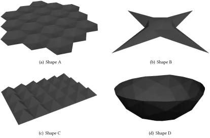
(a) Shape A (b) Shape B (c) Shape C

Figure 3.5:Graph-based camera network deployment.

time expressed in minutes.

Table 3.2:Graph-Based Simulation Results (shape A)

Method Triangles Greedy Optimal Performance Time

Normal 379 10 8 0.9603 6.55

Extended 379 11 8 0.9603 6.89

Table 3.3:Graph-Based Simulation Results (shape B)

Normal 418 19 10 0.9616 9.14

Extended 418 19 10 0.9616 8.71

Table 3.4:Graph-Based Simulation Results (shape C)

Normal 114 24 24 0.7281 0.22

Extended 114 19 19 0.9474 0.23

From the results it can be seen that both methods compute a solution approximately under the same amount of time. When comparing the deployments for shapes A and B, it can be seen that the cost and performance are the same for both methods. However, in the case of shape C the method using the extended solution space outperforms the method using the regular solution space. is evidence is in accordance with the theoretical expectation (see Section Section 3.3). e method using the extended solution space performs equally well, or beer than the method using the regular solution space.

(43)

respect to the number of sensor-lens combinations in the input list. anks to the method described in Section 3.4 the selection of the optics is now done in constant time. Table 3.5 shows a comparison between the execution times using generate-and-test and the new analytic approach. In this case there are a total of ﬁve sensor-lens combinations in the input list.

Table 3.5:Execution Time Comparison for Graph-Based Method

Generate-and-test Analytic approa

Shape A 32.38 min 6.89 min

Shape B 42.67 min 8.71 min

Shape C 01.17 min 0.23 min

3.6.2 Experiments

(a) Cranksha (b) Motor Coupling

Figure 3.6:Graph-based sensor network deployment.

Next, the graph-based method is tested using a physical apparatus. In this experiment, camera conﬁgurations are generated to cover two mechanical parts: a cranksha and a motor coupling, as seen in Figure 3.6. In this case only one type of camera (iCube NS4133BU) and one type of lens (NET SV-0813V) are used; the task parameters were selected as follows: 𝑅 = 𝑅 = 0.4,𝑐 = 1.0,𝑐 = 5.0,

and𝜁 = 𝜁 = 0.9599.

ere is a problem inherent in the positioning of the cameras. Unlike the simulation, human operators are unable to place the cameras at the exact location described by the generated sensor conﬁguration. e solution is to use extrinsic camera calibration as means of feedback and to repeat the process of positioning and calibrating until all cameras are close enough to their respective lo-cations. Although the robotic manipulator in Figure 3.6(b) would have been an ideal solution to this problem, the reach of the robotic arm is too small to eﬀect all camera positions. In this experiment it is reported that the mean euclidean error between the camera locations and the actual locations is

10mm.

(44)

cameras image the part, and the greatest angle at which cameras can see non-parallel faces of the part. ese measurements are reported in Tables 3.6 and 3.7 under “Measured”. e data reported under “Expected” is the result of the simulation aer the sensor conﬁguration was generated.

Table 3.6:Cranksha

Expected Measured

Visibility 96.58% 91.94%

Resolution 0.4mm/𝑝𝑥 0.35mm/𝑝𝑥

Angle 53.10∘ _51.98∘

Table 3.7:Coupling

Expected Measured

Visibility 100% 98.21%

Resolution 0.4mm/𝑝𝑥 0.31mm/𝑝𝑥

Angle 54.74∘ 54.00∘

(45)

Part II

(46)

CHAPTER

4

Tensor Framework

Whether you can observe a thing or not depends on the theory which you use. It is the theory which decides what can be observed.

Albert Einstein (1879–1955)

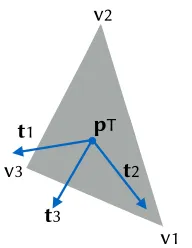
e ultimate goal of modeling the vision system is to be able to predict the system’s performance. is predictive quality may be useful for simulations and optimization, and in terms of the later, the optimal state is deﬁned as follows. A triangle –the atomic unit that represents a task– is optimally imaged by the camera when its centre is at the centre of the viewing frustum, and the normal to its surface is collinear with respect to the optical axis. Figure 4.1 depicts this concept.

0

min(zf, zR)

zn

αv

αh

Figure 4.1:e camera’s viewing frustum and a task represented by a single triangle.

A Measure of Vision Distance for Optimization of Camera Networks

Scholarship at UWindsor

Scholarship at UWindsor

A Measure of Vision Distance for Optimization of Camera

A Measure of Vision Distance for Optimization of Camera

Networks

Networks

A M  V D 

O  C N

Jose Alarcon

A D

S   F  G S

  D  E  C E

 P F   R 

 D  D  P

  U  W

A M  V D  O  C N

Declaration of Previous Publication

Abstract

Acknowledgements

Contents

List of Tables

List of Figures

List of Algorithms

CHAPTER

1

Introduction

1.1 Optimization of Camera Networks

1.2 Motivations

1.2.1 Camera Deployment

1.2.2 Camera Reconfiguration

1.2.3 Camera Selection

1.2.4 Next Best view

1.3 Proposition

1.4 Thesis Outline

Part I

CHAPTER

2

State of the Art

2.1 Overview

2.1.1 Camera Deployment

2.1.2 Camera Reconfiguration

2.1.3 Camera Selection and the Next Best View Problem

2.1.4 Applications of Diﬀerential Geometry

2.2 Modelling the Vision System

¹

CHAPTER

3

Graph-Based Sensor Deployment

3.1 Overview

3.2 The Problem

3.3 The Solution Space

3.3.1 Scene Discretization

3.3.2 Viewpoint Generation

3.3.3 ality of the Solution Space

3.3.4 Extended Solution Space

3.4 Optics Optimization

3.4.1 Hardware Selection

3.5 The Sensor Deployment Algorithm

3.5.1 Graph-Based Data Structure

⋯

⋯

⋮

⋮

⋱

⋮

⋯

3.5.2 Viewpoint Selection

3.5.3 Cost Minimization

3.6 Experimental Validation

3.6.1 Simulations

3.6.2 Experiments

Part II

CHAPTER

4

Tensor Framework