Linear-Phase FIR Digital Filter Design with Reduced Hardware Complexity using Extremal Optimization

(1)

University of Windsor University of Windsor

Scholarship at UWindsor

Electronic Theses and Dissertations Theses, Dissertations, and Major Papers

2016

Linear-Phase FIR Digital Filter Design with Reduced Hardware

Complexity using Extremal Optimization

Manpreet Singh Malhi University of Windsor

Follow this and additional works at: https://scholar.uwindsor.ca/etd

Recommended Citation Recommended Citation

Malhi, Manpreet Singh, "Linear-Phase FIR Digital Filter Design with Reduced Hardware Complexity using Extremal Optimization" (2016). Electronic Theses and Dissertations. 5746.

https://scholar.uwindsor.ca/etd/5746

This online database contains the full-text of PhD dissertations and Masters’ theses of University of Windsor students from 1954 forward. These documents are made available for personal study and research purposes only, in accordance with the Canadian Copyright Act and the Creative Commons license—CC BY-NC-ND (Attribution, Non-Commercial, No Derivative Works). Under this license, works must always be attributed to the copyright holder (original author), cannot be used for any commercial purposes, and may not be altered. Any other use would require the permission of the copyright holder. Students may inquire about withdrawing their dissertation and/or thesis from this database. For additional inquiries, please contact the repository administrator via email

(2)

Linear-Phase FIR Digital Filter Design with Reduced Hardware

Complexity using Extremal Optimization

By

Manpreet Singh Malhi

A Thesis

Submitted to the Faculty of Graduate Studies

through the Department of Electrical and Computer Engineering in Partial Fulfillment of the Requirements for

the Degree of Master of Applied Science at the University of Windsor

Windsor, Ontario, Canada

2016

(3)

Linear-Phase FIR Digital Filter Design with Reduced Hardware

Complexity using Extremal Optimization

by

Manpreet Singh Malhi

APPROVED BY:

______________________________________________ Dr. Guoqing Zhang

Department of Mechanical, Automotive & Materials Engineering

______________________________________________ Dr. Huapeng Wu

Department of Electrical and Computer Engineering

______________________________________________ Dr. Hon Keung Kwan, Advisor

Department of Electrical and Computer Engineering

(4)

iii

DECLARATION OF ORIGINALITY

I hereby certify that I am the sole author of this thesis and that no part of this thesis

has been published or submitted for publication.

I certify that, to the best of my knowledge, my thesis does not infringe upon anyone’s

copyright nor violate any proprietary rights and that any ideas, techniques,

quotations, or any other material from the work of other people included in my

thesis, published or otherwise, are fully acknowledged in accordance with the

standard referencing practices. Furthermore, to the extent that I have included

copyrighted material that surpasses the bounds of fair dealing within the meaning of

the Canada Copyright Act, I certify that I have obtained a written permission from

the copyright owner(s) to include such material(s) in my thesis and have included

copies of such copyright clearances to my appendix.

I declare that this is a true copy of my thesis, including any final revisions, as

approved by my thesis committee and the Graduate Studies office, and that this

thesis has not been submitted for a higher degree to any other University or

(5)

iv

ABSTRACT

Extremal Optimization is a recent method for solving hard optimization problems.

It has been successfully applied on many optimization problems. Extremal

optimization does not share the disadvantage of most of the other evolutionary

algorithms, which is the tendency to converge into local minima. Design of finite

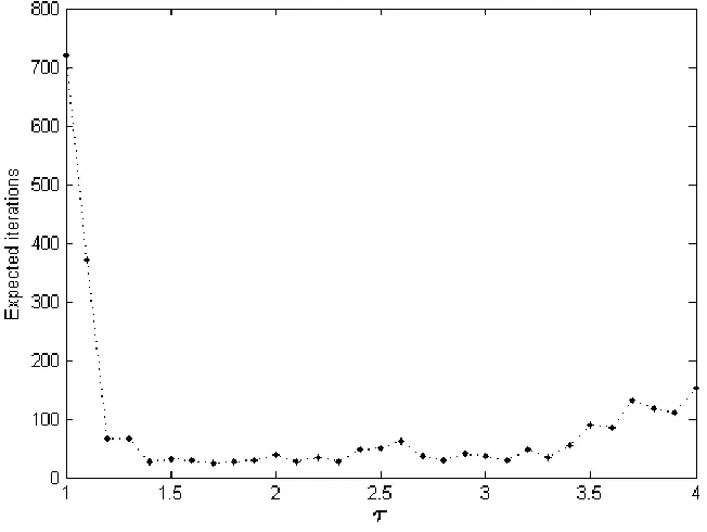
word length FIR filters using deterministic techniques can guarantee optimality at

the expense of exponential increase in computational complexity. Alternatively,

Evolutionary Algorithms are capable of converging very fast to a minimum, but

have higher chances of failure if the ratio of feasible solutions is very less in the

search space. In this thesis, a set of feasible solutions are determined by linear

programming. In the second step, Extremal Optimization is used to further refine

these results. This strategy helps by reducing the search space for the EO algorithm

(6)

v

Dedicated to my mother, who supported me both financially and morally and to

(7)

vi

ACKNOWLEDGEMENTS

I would like to thank Prof. H. K. Kwan for introducing me the subject of digital filter

design using extremal optimization and his guidance and support throughout the

research. I would also like to thank Dr. H. Wu and Dr. G. Zhang for their valuable

feedback and suggestions. And also, Kunwar Rehan for the valuable discussions

(8)

vii

LIST OF TABLES

Table 1.1. Symmetric filters... 5

Table 5.1. Specifications of the benchmark filters ... 59

Table 5.2. Specifications of the Band pass and Band stop filters ... 60

Table 5.3. Filter A coefficients, basis set and its adder synthesis ... 63

Table 5.4. Filter S2 coefficients, basis set and its adder synthesis ... 65

Table 5.5. Filter B coefficients, basis set and its adder synthesis ... 67

Table 5.6. Filter C coefficients, basis set and its adder synthesis ... 70

Table 5.7. Filter Y1 coefficients, basis set and its adder synthesis ... 72

Table 5.8. Filter G1 coefficients, basis set and its adder synthesis ... 75

Table 5.9. Band pass filter coefficients, basis set and its adder synthesis ... 77

Table 5.10. Band stop filter coefficients, basis set and its adder synthesis ... 79

Table 5.11. Comparison of the results with other methods ... 82

Table 5.12. Results of Band-pass and Band-stop filters ... 83

(12)

xi

LIST OF FIGURES

Fig. 1.1. Types of filters based on the frequency response ... 2

Fig. 1.2. FIR filter in direct form ... 3

Fig. 1.3. FIR filter in transposed direct form ... 4

Fig. 1.4. Type I FIR filter coefficients ... 6

Fig. 1.5. Phase response of a linear phase filter ... 7

Fig. 1.6. Filter specifications... 8

Fig. 1.7. Comparison between finite and infinite precision FIR filter responses ... 10

Fig. 1.8. Possible values in a non-uniform quantization scheme ... 13

Fig. 1.9. Frequency response with scaling of the coefficients ... 14

Fig. 1.10. Linear phase type I FIR filter with reduced number of multipliers ... 16

Fig. 2.1. Constant multiplication realization using the algorithm... 25

Fig. 2.2. The adder tree for the above example ... 25

Fig. 4.1. Variation of cost function with iterations ... 37

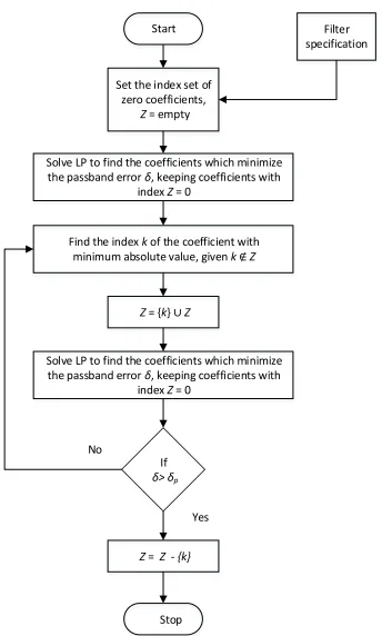
Fig. 4.2. Flowchart of the algorithm ... 38

Fig. 4.3. Extremal optimization algorithm ... 40

Fig. 4.4. Estimating filter order and word-length ... 42

Fig. 4.5. Flowchart of the algorithm for fixing the zero coefficients... 44

Fig. 4.6. Flowchart of the algorithm for partitioning the gain ... 46

(13)

xii

Fig. 5.1. Convergence at 𝜏 = 1.0 ... 53

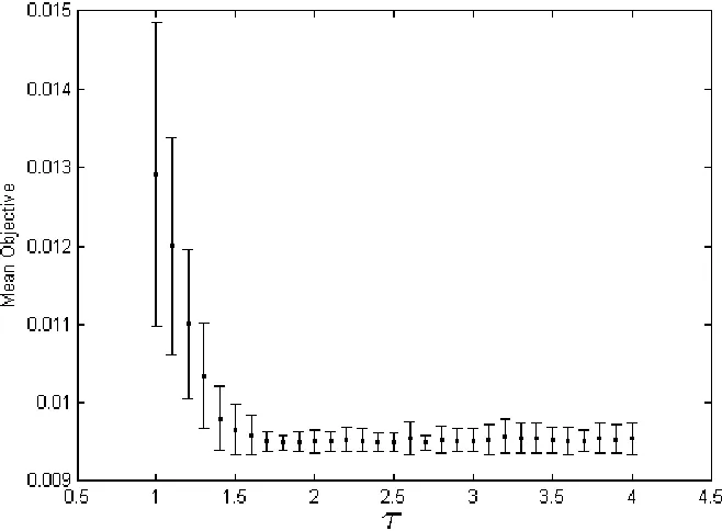
Fig. 5.5. Variation of mean value of objective with 𝜏 ... 56

Fig. 5.6. The variance of the final objective with 𝜏. ... 57

Fig. 5.7. Variance (dots) and mean value (stars, shifted vertically) ... 57

Fig. 5.8. Expected number of iterations at different 𝜏. ... 58

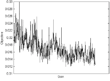
Fig. 5.9. Variation of error of the filter quantized at different gains ... 61

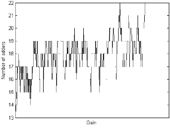
Fig. 5.10. Variation of number of multiplier block adders at different gains ... 62

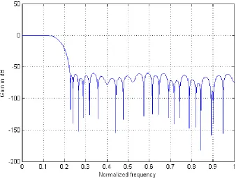
Fig. 5.11. Magnitude response of filter A ... 63

Fig. 5.12 Passband of the magnitude response of filter A ... 64

Fig. 5.13. Magnitude response of filter S2... 66

Fig. 5.14. Passband of the magnitude response of filter S2 ... 66

Fig. 5.15. Magnitude response of filter B ... 68

Fig. 5.16. Passband of the magnitude response of filter B ... 68

Fig. 5.17. Magnitude response of filter C ... 71

Fig. 5.18. Passband of the magnitude response of filter C ... 71

Fig. 5.19. Hardware implementation of filter Y1 ... 73

(14)

xiii

Fig. 5.21. Passband of the magnitude response of filter Y1 ... 74

Fig. 5.22. Magnitude response of filter G1 ... 76

Fig. 5.23. Passband of the magnitude response of filter G1 ... 76

Fig. 5.24. Magnitude response of Bandpass filter ... 78

Fig. 5.25. Passband of the magnitude response of Bandpass filter ... 78

Fig. 5.26. Magnitude response of Band stop filter ... 80

(15)

xiv

LIST OF ABBREVIATIONS/SYMBOLS

ACO b CSA CSD DFT 𝐷(𝜔) 𝛿 𝛿𝑝 𝛿_𝑠 EO EWL 𝐸(𝜔) FIR g GA ℎ_𝑘 𝐻(𝜔) IIR LP MAG MCM MILP MSB N NP NPRM Obj Pmax Pmin

Ant Colony Optimization

Passband gain

Carry Save Adders

Canonical Signed Digit

Discrete Fourier Transform

Desired frequency response

Passband ripple

Specified passband ripple

Specified stopband ripple

Extremal Optimization

Effective Word-length

Weighted error function

Finite Impulse Response

Passband gain

Genetic Algorithm

kth filter coefficient

Frequency response of the filter

Infinite Impulse Response

Linear Program

Minimized Adder Graph

Multiple Constant Multiplication

Mixed Integer Linear Programming

Most Significant Bit

Filter length

Non-deterministic Polynomial Time

Normalized Peak Ripple Magnitude

Objective function value

Maximum absolute value of frequency response in passband

(16)

xv PSO

RAG-n

RCA

SA

Smax

SPOT (SPT)

𝑊(𝜔)

𝜔

𝜔𝑝

𝜔_𝑠

Particle Swarm Optimization

n-Dimensional Reduced Adder Graph

Ripple Carry Adders

Simulated Annealing

Maximum absolute value of frequency response in stopband

Sum of Power of Two

Weighting function

Normalized frequency

Passband cut-off frequency

(17)

1

Chapter 1 Introduction

An analog filter in electronics is used to remove or attenuate certain frequencies from the

input signal and allow others to pass. Digital filters have similar purpose, but they work on

digital signals. A digital filter works by doing mathematical operations on the input signal

and its delayed versions.

The use of digital filters is widespread nowadays due to number of advantages over analog

filters, some of which are shown below:

1. Digital filters can be used to achieve frequency responses which are impossible or

difficult to achieve using analog filters. For example, it is extremely difficult to

construct linear phase analog filters.

2. Digital filters are extremely stable due to their inherent mathematical construction. The

frequency response does not change with time. On the other hand, due to the finite

tolerances involved in the manufacture of electronic components the frequency

response of similar analog filters are never exactly same. Also, the values of capacitors,

resistors, etc. used in the analog filters may change with ageing, resulting in the change

in filter characteristics.

3. Analog filters usually take lots of space for their construction compared to digital

filters.

4. The characteristics of the digital filters can be easily changed by reprogramming, while

an analog filter might need a complete redesign of the circuit.

1.1 Types of filters

1.1.1 Based on the frequency response

Based on the frequency response, the filters can be categorized in the following 4 common

(18)

2

Fig. 1.1. Types of filters based on the frequency response

These are described below:

1. Low pass filter: The low pass filter allows low frequencies to pass while removing the

high frequencies.

2. High pass filter: The high pass filter allows high frequencies to pass while removing

the low frequencies.

3. Band pass filter: The band pass filter allows only a certain band of frequencies to pass.

4. Band stop filter: The band stop filter allows all frequencies to pass except a band

which it removes.

In addition to these basic types, there are other types such as notch filters, comb filters, etc.

The slant part of the frequency response of the filters is called the transition region, in

which the frequency response transitions from the pass band to stop band or vice versa. A

(19)

3 1.1.2 Based on the impulse response

Based on the impulse response, there are 2 categories of digital filters, namely, finite

impulse response (FIR) and infinite impulse response (IIR) filters. As the names suggest,

when an impulse input is given to the FIR filter, the output decays to 0 in a finite amount

of time. On the other hand the output takes infinite amount of time to decay to 0 in the case

of an IIR filter. This is due to the recursive nature of an IIR filter, where the output is fed

back to the filter, resulting in an output even when the input has been stopped.

1.2 FIR filters

Fig. 1.2 shows the direct implementation of an FIR filter. 𝑇 is delay and ℎ₀, ℎ₁… ℎ_𝑁−1 are

filter coefficients. 𝑥[𝑘], 𝑥[𝑘 − 1], … 𝑥[𝑘 − 𝑁 + 1] are the input and the delayed versions

of the input. 𝑦[𝑘] is the output of the filter. It can be noted from the figure that there is no

feedback from the output of the filter.

T

+

. . .

x[k]

y[k]

T

X[k-1] X[k-2] X[k-N+1]

h

0

h

₁

h

₂

h

N-1

+

₊

Fig. 1.2. FIR filter in direct form

The output of the filter can be written in the following equation form:

𝑦[𝑘] = ℎ0𝑥[𝑘] + ℎ1𝑥[𝑘 − 1] + ⋯ + ℎ𝑛−1𝑥[𝑘 − 𝑁 + 1] 1.1

(20)

4 𝐻(𝑧) = ∑ ℎ_𝑛𝑧−𝑛

𝑁−1

𝑛=0

1.2

The frequency response of the filter can be found by substituting 𝑧 with 𝑒𝑗𝜔𝑇 as shown

below, where 𝜔 is the frequency of the input signal.

𝐻(𝑒𝑗𝜔𝑇_{) = ∑ ℎ}

𝑛𝑒−𝑗𝜔𝑛𝑇 𝑁−1

𝑛=0

= ∑ ℎ_𝑛cos (𝜔𝑛𝑇)

𝑁−1

𝑛=0

− 𝑗 ∑ ℎ_𝑛sin (𝜔𝑛𝑇)

𝑁−1

𝑛=0

1.3

Generally, in practical implementations, the direct transposed form is used for the FIR

filter. This has the advantage, as it does not require the extra shift register for the input.

+

. . .

x[k]

y[k]

h

0

h

₁

h

₂

h

N-1

+

T

₊

T

₊

T

Multiplier block

Fig. 1.3. FIR filter in transposed direct form

1.2.1 Linear Phase Filters

The equations 1.1-1.3 represent general FIR filters with arbitrary magnitude and phase

response. It can be shown that it is possible to construct FIR filters with linear phase

response. This is possible when the filter coefficients have an even or odd symmetry.

Depending on the order of the filter and the symmetry of the filter coefficients, the linear

(21)

5

Order Symmetry 𝐻(𝜔)at 𝜔 = 0 𝐻(𝜔) at 𝜔 = 𝜋/𝑇

Type I even even any any

Type II odd even any 0

Type III even odd 0 0

Type IV odd odd 0 any

Table 1.1. Symmetric filters

If ℎ0, ℎ1… ℎ𝑁−1 are the filter coefficients, where 𝑁 is the length of the filter, then the

following relations hold for the coefficients of the different types of filters.

Type I: ℎ𝑘 = ℎ𝑁−𝑘+1, 𝑁 is odd

Type II: ℎ_𝑘 = ℎ_{𝑁−𝑘+1}, 𝑁 is even

Type III: ℎ_𝑘 = −ℎ_{𝑁−𝑘+1}, 𝑁 is even

Type IV: ℎ𝑘 = −ℎ𝑁−𝑘+1, 𝑁 is odd

1.4

The amplitude responses of the four types of the filters can be expressed in the following

equations:

Type I:

𝐻(𝜔) = ℎ(𝑀) + 2 ∑ ℎ𝑛cos ((𝑀 − 𝑛)𝜔) 𝑀−1

𝑛=0

1.5

Type II:

𝐻(𝜔) = 2 ∑ ℎ_𝑛cos ((𝑀 − 𝑛)𝜔)

𝑁/2−1

𝑛=0

1.6

(22)

6 𝐻(𝜔) = 2 ∑ ℎ_𝑛sin ((𝑀 − 𝑛)𝜔)

𝑀−1

𝑛=0

1.7

Type IV:

𝐻(𝜔) = 2 ∑ ℎ𝑛cos ((𝑀 − 𝑛)𝜔)

𝑁/2−1

𝑛=0

1.8

Where, 𝑀 = (𝑁 − 1)/2

It can be seen that Type I can be used to construct both low and high pass filters, Type II

can be used to construct only low pass filters, Type IV can be used to construct only high

pass filters and Type III can be used to construct only band pass filters. Due to this, Type

I filters are most common.

In the following figure, coefficient values of a Type I linear phase filter are shown:

(23)

7

The coefficients are symmetric around the central coefficient, as can be seen in the above

figure.

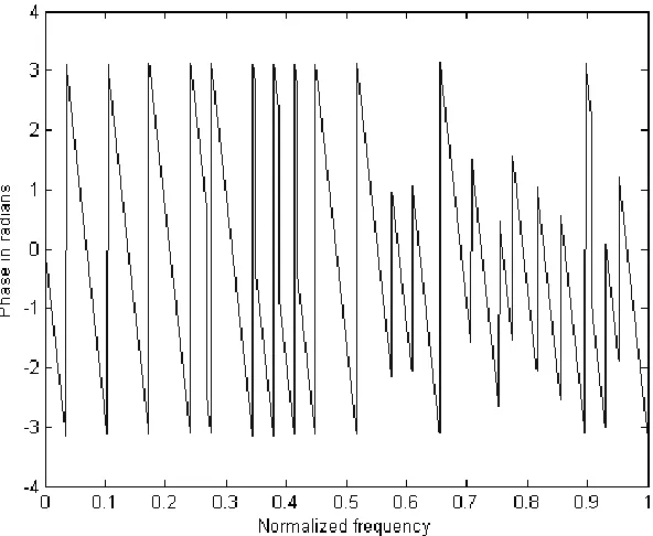
The phase response of a linear phase filter is shown in the following figure:

Fig. 1.5. Phase response of a linear phase filter

We can see that the phase response of the filter varies linearly. The discontinuities are due

to two reasons:

1. 2𝜋 + 𝜃 = 𝜃, resulting in the phase being confined from−𝜋 to 𝜋.

2. The sign reversal of the frequency response.

1.3 Design of FIR filters

FIR filters can be designed using various methods. The most common of these methods

(24)

8

1. Equi-ripple (minimax) design in which the maximum frequency response error from

the specified frequency response is minimized. Parks-McClellan method can be used

to design FIR filters based on minimax criterion.

2. Least mean square design, in which the mean square error is minimized from the

desired frequency response.

3. Window-based methods based on inverse DFT.

Here, we will focus on the minimax design of FIR filters, as this is the criterion on which

the work in this thesis is based.

1.3.1 Equi-ripple design of linear phase FIR filters

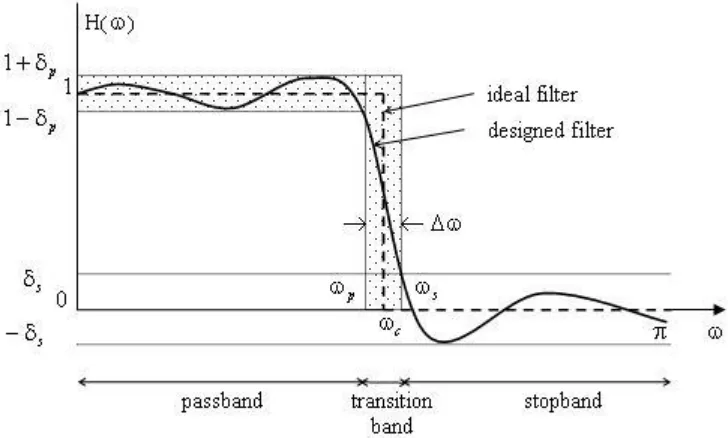
The specifications of the filter are given, before it is designed. Fig. 1.6 shows the

specifications of a low-pass filter, which is to be designed based on equi-ripple method.

Fig. 1.6. Filter specifications

The broken plot represents the desired filter response, which corresponds to an ideal

low-pass filter, with cut-off frequency 𝜔_𝑐. The response is exactly 1 in the passband and drops

to 0 in the stopband sharply. In practical filters of finite length, the frequency response

deviates from the ideal response as shown in the solid curve in the figure. Therefore, the

(25)

9

The interval 0-𝜔_𝑝 is the pass-band and 𝜔_𝑐-1 is the stop-band of the filter. For the designed

filter, in the pass-band, the response can vary from 1-𝛿𝑝 to 1+𝛿𝑝 and in the stopband from

-𝛿_𝑠 to 𝛿_𝑠. In the transition region, which is from 𝜔_𝑝 to 𝜔_𝑠 the response can take any value.

𝛿_𝑝 is called the pass-band ripple and 𝛿_𝑠 the stop-band ripple. The tighter the filter

specifications are, the higher the filter length, 𝑁 is required to design the filter.

The above design problem can be formulated as a linear program shown in the following

equations:

Minimize 𝛿

Such that: 1 − 𝛿 ≤ 𝐻(𝜔) ≤ 1 + 𝛿, for 𝜔 ∈ [0, 𝜔_𝑝]

−(𝛿_𝑠𝛿)/𝛿_𝑝 ≤ 𝐻(𝜔) ≤ (𝛿_𝑠𝛿)/𝛿_𝑝, for 𝜔 ∈ [ 𝜔_𝑠, 1]

1.9

Where, 𝐻(𝜔) is the frequency response of the filter and is given by

𝐻(𝜔) = ∑ ℎ(𝑛)Trig(𝜔, 𝑛)

⌊𝑁−1₂ ⌋

𝑛=0

1.10

Where N is the filter length and Trig is a trigonometric function depending on the type of

the filter and whether the filter length is odd or even (See equations 1.5-1.8).

Solving the linear program (LP), we can find the values ofthe filter coefficients ℎ(𝑛) and

the ripple 𝛿.

The filter can be instead designed using Parks-McClellan method which is very efficient.

This is an iterative algorithm, reducing the maximum error in each iteration. The MATLAB

function firpm is based on the Parks-McClellan method and can be used to design

linear-phase FIR filters with a given length and specified pass and stop bands. The syntax of the

(26)

10 b = firpm(n,f,a,w)

where, n is the filter order, which is one less than the filter length,

f and a define the pass and stop bands. For example, f = [0 0.3 0.5 1], and a = [1 1 0 0]

represents a low pass filter with pass band from 0 to 0.3𝜋 and stop band from 0.5𝜋 to 𝜋.

w is the weight vector of length equal to the number of bands. Each value in the vector

represents the weight assigned to the corresponding band of the filter.

1.3.2 Effect of finite precision

In practice due to the finite length of registers in processors, a filter with continuous filter

coefficients is not possible to implement. The coefficients must be represented by numbers

of finite word-length. This affects the frequency response of the filter negatively.

Fig. 1.7. Comparison between finite and infinite precision FIR filter responses

In Fig. 1.7 the blue solid plot represents the response of an optimal un-quantized filter

(27)

11

constant. After the filter coefficients are quantized to an effective word-length (EWL) of

10 bits excluding the sign bit, the frequency response is again plotted and is shown in green,

dashed graph. It is seen that even with 10 bits EWL, there is a significant distortion in the

frequency response of the filter, which is clearly noticeable in the stop band of the response.

In addition, the equi-ripple character of the response is lost.

1.4 Quantization of coefficients

The continuous filter coefficients can be quantized using either uniform quantization or

non-uniform quantization. The uniform quantization can be achieved by the following

number representations:

1.4.1 Signed magnitude representation

In this representation the magnitude of the number is represented by the bits excluding the

MSB and the sign of the number is represented by the MSB.

For example: (0101)2 = +510 and (1010)2 = -210

The number 0 has 2 possible representations in this system, which are (0000)2 and (1000)2.

1.4.2 One’s compliment representation

In this representation the negative of a number is equal to bitwise OR of the number.

For example: (0110111)2 = +5510 and (1001000)2 = -5510

In order to add two one’s compliment numbers, it is necessary to add the end-around carry

to the result to obtain the correct answer. For example:

(1110001)2 + (0010000)2 = (1 0000001)2

To obtain the correct answer the carry bit is added to the remaining number, which gives

(28)

12 1.4.3 Two’s compliment representation

To avoid the task of adding the carry bit after the addition of two one’s compliment numbers, in the two’s compliment representation the negative of a number is formed by

taking bit-wise not of the number and then adding 1 to the result.

For example: -5510 is represented by (1001000)2 + (1)2 = (1001001)2

The addition of two 2’s compliment numbers is straightforward and can be done using

normal addition.

1.4.4 Signed digit format

In signed digit format each digit of the number has a sign associated with it. One example

is balanced ternary, whose base is 3 and the digits can take the values from {-1, 0, 1}.

For example: (1 0 -1 -1)2 = 23 - 21 -20 = 8 – 2 – 1 = 5

The signed digit format is not unique.

1.4.5 Canonical signed digit representation

If in the signed digit representation no two consecutive digits are non-zero, then the

resulting representation is called canonical signed digit representation (CSD). The CSD

representation of a number is unique.

1.4.6 Non-uniform quantization

There are a number of quantization representations in which the difference between 2

consecutive values in the range of the representation does not remain uniform. An example

is limiting the number of signed non-zero digits in the representation of the filter

coefficients. Limiting the number to 2, the filter coefficients are then represented by the

following equation

ℎ_𝑛 = 𝑐_𝑛12−𝑏𝑛1_{+ 𝑐}

(29)

13 Where,

𝑐𝑛1, 𝑐𝑛2∈ {−1,0,1} and 𝑏𝑛1, 𝑏𝑛2∈ {1,2, … 𝑏}

A plot of the values which ℎ_𝑛 can take is shown in the Fig. 1.8.

Fig. 1.8. Possible values in a non-uniform quantization scheme

As can be seen, the values are closely spaced near 0 and the gaps between the values

generally increases near -1 and 1. Therefore, quantizing larger coefficients results in large

quantization errors.

1.4.7 Integer representation of coefficients

The coefficients are quantized to a certain number of bits in an algorithm. The number of

digits in binary format of a coefficient, proceeding initial zeros, after quantization is called

the effective word-length of the coefficient. For example, consider a filter with 3

coefficients with values 0.4569, -0.2438 and 0.1211. The binary values of these coefficients

are

0.01110100111101110110…, -0.00111110011010011010… and

0.00011111000000000110…

If these are rounded to 9 digits after the binary point, then the values become

0.011101010, -0.001111101 and 0.000111110

The EWL of each coefficient is then equal to the number of digits of each coefficient after

(30)

14

Instead of working on these values which are binary, these can be multiplied by a number

which is a power of 2, i.e. 2n, such that the resulting values become integers. In the above

example, it can be easily seen that this number is 29. Multiplying the coefficients with 29,

we get

11101010, -1111101 and 111110, which in decimal are 234, -125 and 62.

1.5 Normalized Peak Ripple Magnitude (NPRM)

The equations 1.5-1.8 give the frequency response of the filters. It can be noted that if all

the coefficients of the filter are multiplied by a constant K, then the resulting frequency

response is identical to the original response except that it is scaled by a factor of K. This

is not important in most of the applications, as the filtered signal can be passed through an

amplifier with gain 1/K, to cancel the scaling factor. Therefore, in the binary representation

of filter coefficients, if all the coefficients are shifted left or right by same number, i.e. they

are multiplied by 2, 4, 8, , etc., the resulting filter remains equivalent to the original filter.

(31)

15

In Fig. 1.9 blue solid plot represents frequency response of a filter with unity passband

gain. If the coefficients are multiplied by 1.5, the frequency response of the resulting filter

is identical but scaled by a factor of 1.5, as shown in green dashed line. And similar is the

case with scaling with 0.7.

Consider the example given in section 1.4.7, where the coefficients are scaled to integers.

The largest coefficient is 234. But it can be easily seen that if the coefficients were scaled

such that the largest coefficient lies between 128 and 255, even then the EWL of the filter

would remain the same. In other words, if ℎ_𝑚𝑎𝑥 is the largest coefficient in terms of

magnitude and EWL is the effective word-length, then the gain of the scaled filter can be

varied from 2

𝐸𝑊𝐿−1

ℎ𝑚𝑎𝑥 to 2𝐸𝑊𝐿 ℎ𝑚𝑎𝑥.

Therefore, it is possible that the optimum filter is realized while searching in the

neighborhood of filters quantized using gain other than 1. Therefore while optimizing the

filter coefficients the gain can be allowed to change. In order to do this, the optimization

problem is defined as below:

minimize: 𝛿 𝑔⁄ = 1

𝑔max𝜔∈𝐹|𝐸(𝜔)| 1.12

Where, 𝐹 is a set of frequency points excluding the transition bands.

And, 𝐸(𝜔) = 𝑊(𝜔)(𝑔𝐷(𝜔) − 𝐻(𝜔)) 1.13

Where, 𝐷(𝜔) is the desired frequency response, which is 1 in passbands and 0 in

stopbands, 𝐻(𝜔) is the frequency response of the designed filter and 𝑊(𝜔) is a weighting

function. The weighting function is used to give different weights to different frequencies.

The quantity_{𝛿 𝑔}⁄ is called the Normalized Peak Ripple Magnitude (NPRM) of the filter.

(32)

16 𝑔 =𝑃𝑚𝑎𝑥 + 𝑃𝑚𝑖𝑛

2 if

𝑃_𝑚𝑎𝑥− 𝑃_𝑚𝑖𝑛

2 > 𝑆𝑚𝑎𝑥

𝑔 = 𝑆_𝑚𝑎𝑥 + 𝑃_𝑚𝑖𝑛 if 𝑃𝑚𝑎𝑥 − 𝑃𝑚𝑖𝑛

2 < 𝑆𝑚𝑎𝑥

1.14

Where, 𝑃_𝑚𝑎𝑥 is the maxima of the frequency response in the pass-band, 𝑃_𝑚𝑖𝑛 is the minima

of frequency response in the pass-band and 𝑆_𝑚𝑎𝑥 is the maxima of frequency in the

stop-band.

1.6 Reduced hardware complexity designs

Fig. 1.2 and 1.3 show two forms of hardware implementations of FIR filters. For

linear-phase filters the complexity can be further reduced by utilizing the fact that half of the

coefficients have same magnitude as the other half. The following figure shows type I filter

in transposed direct form, where only the distinct coefficients are used as multipliers,

+

. . .

x[k]

h

0

h

1

h

2

h

(N-1)/2-1

+

T

₊

T

₊

T

Multiplier block

+

T

+

T

+

T

y[k]

Fig. 1.10. Linear phase type I FIR filter with reduced number of multipliers

1.6.1 Using CSD coding of the coefficients

The coefficients can be converted into CSD format. As CSD representation has minimum

number of non-zero binary digits, therefore the complexity of the multiplier block is

(33)

17 1.6.2 Reduced adder graph designs

Although using CSD instead of simple multipliers can reduce the adder complexity in the

multiplier block, yet it is possible to further reduce the number of adders by utilizing the

common additive factors among the coefficients. For example the coefficients 5, 9 and 23

can each be realized using 1, 1 and 2 adders (4+1, 8+1 and 32-8-1) respectively, requiring

total of 4 adders. But if 23 is realized by utilizing the previously realized coefficients (5

and 9) as 2×9+5, then only 1 adder is required for synthesizing 23. (Note that multiplying

by 2 requires only shifts and has negligible hardware requirement). Various algorithms

[2]-[5] has been developed to find the optimal adder graph, some of which are explained in

chapter 2.

1.7 Motivation

The focus of the thesis is the design of linear phase FIR filter which satisfies the given

design specifications and also tries to achieve minimum number of hardware adders

required for the multiplierless design. In the literature, there are algorithms which can

design optimum filters having minimum number of adders, but the run-time of these

algorithms usually increases exponentially as the length of the filter to be designed is

increased. On the other hand there are some algorithms based on evolutionary methods

which can design the filters in relatively less time but the number of adders of the designed

filter is usually far from optimum.

In this thesis, the recently proposed Extremal Optimization (EO) is used to design such

filters trying to achieve near optimum results and on the other hand avoiding the

exponential increase in run-time as the filter length increases.

1.8 Thesis organization

The rest of the thesis report is organized as follows:

In the second chapter, the literature is reviewed focusing on some of the state of the art

methods for designing linear phase FIR filters. Some of the important deterministic and

(34)

18

minimum adder multiplier graphs, such as [2] and RAG-n [4] are explained. In addition,

some techniques used to reduce the search space and making the linear program based

calculation of the filter coefficients faster are reviewed

In the third chapter, the theoretical background of the extremal optimization (EO) method

is given. Also, some major improvements such as 𝜏-EO and population based EO are

discussed.

In the fourth chapter, the proposed method is explained in detail. Various steps used in the

algorithm like reducing the search space, partitioning the gain and the methods used to

speed-up the calculations are discussed.

In the fifth chapter, the analysis of the convergence characteristics of the algorithm is done.

Some benchmark filters are designed using the algorithm and their multiplier blocks are

synthesized and shown. The run-time of the algorithm is also calculated and discussed and

a comparison is made with the state of the art methods.

In the sixth chapter, the conclusion is given.

1.9 Main contributions

The main contribution of the work done here is the implementation of EO algorithm and

adapting it to make it suitable for designing FIR filters. The algorithm has not been

previously used for the design of digital filters. The disadvantage of other algorithms such

as GA and PSO is that they require fine tuning of the parameters. Also there is a problem

of early convergence to a local minimum. EO on the other hand has just one adjustable

parameter, which is relatively easy to tune. Also, it is easy to tune EO such that it doesn’t

get trapped in local minima, although at the cost of increasing the runtime.

A specific technique is also developed to make the algorithm fast. The frequency response

is not calculated entirely for each objective function evaluation. Instead, only the

(35)

19

Chapter 2 Review of Literature

Multiplierless digital filters can be realized without the use of multipliers by a shift and add

network and thus are efficient in terms of hardware complexity and power consumption.

The design goal is to minimize the number of adders. There are both deterministic as well

as heuristic methods available for designing finite word length filters. Deterministic

methods based on tree search are able to find the optimum solutions but consume lots of

time if the filter length is high.

Initially, the design of finite word length filters was concentrated on reducing the

representation of filters coefficients. The canonic signed digits (CSD) and Signed Power

of Two (SPOT) representation of numbers was utilized to minimize the bits needed to

represent the filter coefficients. The minimal bit representation led to a reduction in the

number of adders needed to implement the filter either using ripple carry adders (RCA) or

using carry save adders (CSA). The RCA topology required less chip area and consumed

less power but at the expense of reduced operating frequency. The CSA topology increased

the speed at the expense of additional hardware. However, both the topologies had minimal

adder counts under the SPOT design criteria.

With time, research efforts in finite word length filter design drifted towards developing

efficient multiple constant multiplication (MCM) algorithms. The FIR filter in its

transposed direct form could be modelled as a case of MCM wherein the input is multiplied

by all the filter coefficients and then saved in registers and added along the delay line. The

MCM algorithms utilized the redundancies in the filter coefficients and modelled the shift

and add network as a one-input-M-output network (M being the number of unique filter

coefficients). The MCM algorithms were either graph based [3]-[4], or were pattern based

[2].

MCM algorithms produced the minimal adder count for a given set of filters coefficients

but given a filter specification, the coefficient set that can meet the requirement is not

(36)

20

problem and the implementation were consolidated. This led to the dynamically expanding

subexpression space design methods.

Deterministic methods based on tree search are able to find the optimum solutions at the

expense of exponential computational complexity [6]. Thus, design of large order and high

word length filters becomes infeasible. The research in deterministic methods is being

carried out to reduce the search space by excluding the section of the search space from the

algorithm that shows no promise of feasible solutions. However, the exponential

computational growth is unavoidable in all tree search methods and a polynomial time

algorithm can only be guaranteed if every node produces only one child. In [7], a method

is proposed whose runtime is polynomial with the filter length. In this method the passband

gain is divided into large number of sections. In each section a solution is found by

successively finding the feasible range of a coefficient and fixing it the value near the

middle of the range. A feasible solution is chosen which results in minimum number of

adders.

In heuristic methods for designing finite word length filters, the most common strategy is

to find an initial solution, for example by rounding the continuous solution or by finding

an initial good solution with greedy optimization and then search using small number of

values around the rounded values. Totally random search with no initial solutions can only

yield feasible solutions for filter orders less than 30. The shift and add network can be

constructed using MCM algorithms and the objective function is created to direct the search

for finding minimal adder coefficients.

2.1 Filter design algorithms

In the following section some important deterministic and heuristic algorithms from

literature are reviewed.

2.1.1 Deterministic algorithms

1. In [8], a branch and bound algorithm (called FIRGAM) is proposed for the design of

hardware efficient filters. The algorithm designs filters with reduced number of SPT terms.

(37)

21

and fixing the coefficient first to the quantization value nearest to the center of the feasible

range. After a coefficient has been fixed the feasible range of the next coefficients is

recalculated and the same procedure is repeated until all the coefficients has been

successfully quantized.

The number of SPT terms of the solution are calculated and the algorithm then goes through

the search space again to find if a solution with lesser number of SPT terms can be found.

If the feasible range of any coefficient is found to be empty at any stage, the algorithm

backtracks to the previous quantized coefficient and quantizes it to the next nearest

quantization value from the center of its feasible range.

2. [6] proposes an algorithm to design optimum filters in terms of the number of adders.

The method involves mixed integer linear programming (MILP). The filter coefficients are

synthesized based on a dynamically expanding subexpression space.

First, the lower and upper bound of each coefficient is calculated. This is done by solving

the following linear program problem:

minimize: 𝑓 = ℎ(𝑘) and 𝑓 = −ℎ(𝑘)

such that: 𝑏 − 𝛿 ≤ 𝐻(𝜔) ≤ 𝑏 + 𝛿, for 𝜔 ∈ [0, 𝜔_𝑝]

− (𝛿_𝑠𝛿) 𝛿⁄ _𝑝 ≤ 𝐻(𝜔) ≤ (𝛿_𝑠𝛿) 𝛿⁄ _𝑝, for 𝜔 ∈ [𝜔_𝑠,𝜋]

𝑏𝑙 ≤ 𝑏 ≤ 𝑏ℎ

2.1

Where, 𝑏 is the passband gain and 𝛿𝑝 and 𝛿𝑠 are the maximum allowed pass and stop-band

ripple. 𝐻(𝜔) is the magnitude of the frequency response of the filter.

After this a depth first search is done and filter coefficients are fixed to integers one by one.

Once a coefficient is fixed the remaining un-quantized one are re-optimized.

This algorithm is guaranteed to return optimum set of filter coefficients, but for filters with

high word-lengths, the algorithm takes very long time to finish the search and becomes

(38)

22

3. In [7], a polynomial time algorithm is proposed. The method is inspired from FIRGAM

[8] algorithm. In contrast to FIRGAM, the proposed method fixes each coefficient to the

middle of its range and does not try to expand the search in the neighboring values.

As the runtime of linear program is polynomial in number of filter coefficients and the

number of linear programs to be solved also increases linearly with the number of the filter

coefficients, therefore the above algorithm is polynomial in runtime.

In this algorithm, first some of the coefficients are fixed to 0 before proceeding with the

remaining algorithm. The reason is that, if a coefficient is 0, then there is an immediate

reduction in two adders in the delay chain.

After this, the passband gain is divided into number of partitions and the tree search

algorithm, as in [8], is used to fix successively the coefficients to the middle of their feasible

range. The filter coefficients from each gain are synthesized using an MCM algorithm [2]

and the one which yields the result with minimum number of adders is chosen as the final

solution.

4. [9] proposes a polynomial time algorithm which optimizes the coefficients in two steps.

The first step is similar to the one proposed in [7]. After the initial solutions for each gain

are obtained, the ones which are feasible are selected for the second step of the

optimization.

In the second step the coefficients are divided into groups. Each group has 20 coefficients

(the last group might have less than 20 coefficients). Each group is optimized one by one

using a tree search algorithm similar to [6]. Expanding subexpression technique is used to

synthesize the coefficients as they are constructed to yield minimum number of adders.

Once all the groups have been optimized, the process is repeated again several times

starting from the first group. After 2-3 iterations the algorithm converges. The solution at

the gain which yields the best result in terms of number of adders is chosen as the final

solution.

The above algorithm is capable of finding solutions which, in most of the cases, are optimal

(39)

23 2.1.2

Heuristic

algorithms

1. In [10], GA is used to design FIR filter with coefficients which are constrained to the

sums of two numbers, which are powers of two. In order to constrain the search space, a

specific coefficient coding scheme is used. Instead of coding the values of the coefficients

directly, the differences from some leading values are chosen and coded. The leading

values are chosen as the coefficients obtained after quantizing the optimal continuous

coefficients. In the case, when sum of power of two terms (SOPT) is used, the quantization

is done such that the quantized value is the nearest value in the domain of SOPT from the

continuous value.

As the optimal discrete filter coefficients are generally relatively not far away from the

continuous filter coefficients, therefore the differences to be encoded are not very large and

can be encoded using lesser number of bits, compared to encoding the full coefficient

values.

2. In [11], a genetic algorithm is proposed for the design of multiplierless filters. In this

paper the search space is partitioned into a number of search spaces. This is done by

dividing the passband gain into a number of partitions, such that the EWL remains same

as specified. The continuous filter is constructed for each of the partition. Then a search

space is constructed around each solution and GA is used to find feasible solution in this

space having minimum hardware adders. The search space around the nth coefficient is

defined in the following way:

ℎ_𝑞𝑚𝑢 _{(𝑛) = ℎ} 𝑞𝑚

′ _{(𝑛) + 2}𝑐𝑒𝑖𝑙(𝐵𝑚(𝑛)/3)_{− 1}

ℎ𝑞𝑚𝑙 (𝑛) = ℎ𝑞𝑚′ (𝑛) − 2𝑐𝑒𝑖𝑙(𝐵𝑚(𝑛) 3⁄ )+ 1

2.2

Where, ℎ𝑞𝑚′ are the quantized coefficients scaled to integers. ℎ𝑞𝑚𝑢 is the upper limit of the

coefficients and ℎ𝑞𝑚𝑙 is the lower limit of the coefficients. 𝐵𝑚(𝑛) is the EWL of the nth

coefficient.

3. Another GA based algorithm is proposed in [12] for the design of multiplierless filters.

(40)

24

convergence of the algorithm and also avoids the good solutions to be cast away. The gain

is divided into a number of partitions as in [11]. In the second part of the paper the

algorithm is used to design filters in cascade form.

4. In [13] a two stage algorithm is proposed with sums of SPT terms. In the first stage, a

time domain method is used to assign SPT terms to the filter coefficients. In the second

stage a Verterbi’s algorithm type method is used. The problem is cast as dynamic

programming and a trellis search is done to iteratively add SPT terms one by one. The

number of adders are further reduced by using a subexpression sharing method to exploit

the redundancies among the coefficients.

5. A gradient based method, is used in [1]. In this method, the gradient information is

calculated and used to direct the search. The search is directed towards low gradients routes

first and when further improvement stops, the search is redirected to the steeper routes. The

method is semi-random in nature and has low computational cost.

2.2 MCM algorithms

In the following sub-sections two important MCM algorithms for designing multiplierless

realizations of filter coefficients are explained.

2.2.1 MCM algorithm of A. Yurdakul and G. Dündar [2]

There are a number of algorithms in the literature to find the multiplierless realizations of

filter coefficients. RAG-n and C1 algorithms are notable for producing realizations with

optimal number of adders in most of the cases. But these algorithms suffer from the

disadvantage of large memory requirements due to the use of large lookup tables. Also,

when the word-length is higher, the lookup tables become prohibitively large. In this case,

the algorithms can still construct these coefficients using heuristics, but do not guarantee

the optimal number of adders. A fast and efficient algorithm has been introduced in [2]. It

has pseudo-polynomial run-time and memory requirements in the worst case scenario.

The algorithm is based on pattern search in the binary or CSD values of the coefficients.

The pattern search is done at length of 2 throughout the algorithm. Pattern length is defined

(41)

25

word-length 8 is given as 11010110. Then, 1001 and 101 shown in bold as 11010110 and

11010110 respectively are patterns of length 2, whereas 1101 and 100101 are patterns of

length 3 shown in bold as 11010110 and 11010110 respectively. The algorithm iteratively

combines 2 non-zero terms to generate all the coefficients. The step by step realization of

constant multiplication is shown in the following figure:

Step 1:

Step 2:

Step 3:

1 0 1 0 1 0 0 1 0 1 0 1 0 0 1

Step 4:

0 0 t2 0 0 0 0 t1 0 1 0 0 0 0 t1

0 0 0 0 0 0 0 t4 0 0 0 0 0 0 t3

0 0 0 0 0 0 0 0 0 0 0 0 0 0 t5

Fig. 2.1. Constant multiplication realization using the algorithm.

+

1 4 1 8 5×2^5 9 2^5 9 169×2^7 41 21673

Fig. 2.2. The adder tree for the above example

From the figure, we can see that the number of adders required for the synthesis is 5.

2.2.2 RAG-n algorithm

RAG-n algorithm [4] synthesizes the coefficients in two steps. The first part of the

algorithm is optimal and the second part is heuristic. If the algorithm is able to synthesize

all the coefficients in the first step, then the synthesized set is guaranteed to be optimal.

The algorithm uses a lookup table constructed by MAG algorithm. The lookup table

contains the minimum adder graphs of all the integers up to a certain cost, where cost is

the number of additions or subtractions required to synthesize that number. Only the odd

(42)

26

multiplying with 2, which is cost-free. For example, 2, 4, 8, and so on have cost 0 as these

can be constructed without any adders. 3, 5, 7, 9, etc. have cost 1 as they require one adder

for their synthesis as shown below:

4 - 1 = 3, 4 + 1 = 5, 8 - 1 = 7, 8 + 1 = 9

The basic steps of the algorithm are as follows:

 First, all the coefficients are reduced to odd-fundamentals. This is done by making any

negative coefficients positive. Then making the coefficients odd by successively

dividing by 2.

 Any repeated values are removed. The values 0 and 1 are also removed from the set.

 All the odd-fundamentals which have cost 1 are removed from the set. The set of remaining fundamentals is called incomplete set. The number of adders used until now

is the number of fundamentals removed. The set of removed fundamentals is called

complete set.

 Use the complete set and try to construct fundamentals in the incomplete set by adding

two coefficients from the complete set and their multiples with power of 2. The

fundamentals which are able to be constructed in this step are added to the complete

set and removed from the complete set.

 The step 4 is repeated until there are no more fundamentals in the incomplete set or no

more fundamentals in the incomplete set can be constructed.

If by this time the incomplete set is empty then the algorithm stops and the resulting

synthesis is optimal, otherwise the remaining fundamentals are constructed using the

second part of the algorithm which is heuristic.

As the number of coefficients increases for a given word-length the chances of a set

constructed by the algorithm to be optimal increases. For example, when the word-length

is 8, the chances of optimal set are already more than 50% with a set size of around 10 and

almost 100% with a set size of 20. On the other hand, when the word-length is 12, around

(43)

27

2.3 Speeding up the linear program

The maximum number of extrema (i.e. maxima and minima) in the frequency response of

a filter of length 𝑁 is equal to

𝑁_𝑒𝑥𝑡 = ⌊𝑁 + 1

2 ⌋ 2.3

The above number includes the points at frequencies 𝜔 = 0 and 𝜋, but does not include

the frequencies at the edge of the transition bands.

The filter coefficients for a low pass filter with pass and stop band cut-off frequency 𝜔_𝑝

and 𝜔𝑠 respectively, can be evaluated by solving the following linear program

minimize: 𝛿

subject to: 1 − 𝛿 ≤ 𝐻(𝜔) ≤ 1 + 𝛿, for 𝜔 ∈ [0, 𝜔_𝑝]

−𝛿𝑠

𝛿_𝑝𝛿 ≤ 𝐻(𝜔) ≤ 𝛿_𝑠

𝛿_𝑝𝛿, for 𝜔 ∈ [𝜔𝑠, 𝜋]

2.4

Where, 𝛿𝑠

𝛿𝑝 is the ratio of stop and pass band error tolerances and 𝐻(𝜔) is the frequency

response of the filter.

In order to account for all the frequencies, the number of points on the frequency grid need

to be as large as possible. If the number of points is very large, then the number of

constraints of the LP is also very large, which can create instability in the solving algorithm

and also require large computational time. It can be noticed that the only points where

optimization is required are the extremal points on the frequency response. The problem is

(44)

28

In [14], a method, similar to the one used in Parks-mcCllellan is used to solve the above

equations. The algorithm is explained below:

1. 𝑁𝑒𝑥𝑡 number of points are initially chosen in the pass and stop band which are

roughly equally spaced.

2. The equations are solved at these points, in addition to pass and stop band cut-off

frequencies, to get filter coefficients.

3. Frequency response is evaluated using these filter coefficients at roughly 2𝑁

equally spaced points on the frequency grid.

4. Newton’s extrapolation method is applied to accurately determine the extrema of

the frequency response, which are the new 𝑁_𝑒𝑥𝑡 number of points.

5. The steps 2-4 are repeated until the change in the extrema points is less than a given

tolerance.

2.4 Reducing the search space

If the magnitude of the coefficients are quantized to an 𝐸𝑊𝐿 of 𝐵 bits and the filter length

is 𝑁, then the total number of possible filter realizations are equal to (2𝐵+1)𝑁_{= 2}(𝐵+1)𝑁_.

Even for a moderate word-length of 8 and filter length 31, the number of possibilities

is 2279_{≈ 10}84_{, which is enormous. It is impossible to check each and every possibility by}

Brute force to optimize the filter.

A large majority of these possibilities give filters which deviate greatly from the desired

frequency response. The optimum filter coefficients lie close to the quantized filter

coefficients. Therefore it makes sense to look for the optimum filter coefficients in the

vicinity of the quantized filter coefficients. For example in [10], a neighborhood is selected

around each coefficient, which is much less than the full range of the given coefficient.

This way each filter’s neighborhood is encoded with a number of bits which is less than

the 𝐸𝑊𝐿 of the given coefficient. In this way the search space is drastically reduced.

Instead of quantizing the coefficients and then defining an arbitrary search space as

(45)

29

which satisfy the given filter specifications. This is done by solving the following LP for

each of the coefficients. To find the feasible range of ith coefficient, solve

minimize: 𝑓₀ = ℎ(𝑖) and 𝑓₁ = −ℎ(𝑖)

subject to: (1 − 𝛿_𝑝) ≤ 𝐻(𝜔) ≤ (1 + 𝛿_𝑝), for 𝜔 ∈ [0, 𝜔_𝑝]

−𝛿_𝑝 ≤ 𝐻(𝜔) ≤ 𝛿_𝑝, for 𝜔 ∈ [𝜔_𝑠, 𝜋]

2.5

Where, 𝐻(𝜔) = ∑⌊ ℎ(𝑛)Trig(𝜔, 𝑛)

𝑁−1 2 ⌋ 𝑛=0

The above equations represent two linear programs, one minimizing 𝑓₀ = ℎ(𝑖) and the

other minimizing 𝑓0 = −ℎ(𝑖). The results of these give the minimum and maximum value

of the ith coefficient. The search space of the filter can now be limited to the feasible range

(46)

30

Chapter 3 Extremal Optimization

Extremal Optimization is a recent heuristic method inspired by models of co-evolution

such as Bak-Sneppen model [19]. It is one of many evolutionary algorithms, such as

Genetic Algorithm (GA), Ant Colony Optimization (ACO), Particle Swarm Optimization

(PSO), Artificial Bee Colony Optimization, etc. Evolutionary algorithms can successfully

optimize a wide variety of optimization problems as they do not make any assumptions

about the underlying fitness landscape of the problem. Therefore, these have been widely

used in the optimization of engineering problems, which are otherwise very difficult to

solve due to the complex nature of the fitness landscape, or due to the huge size of the

search space which is intractable with other algorithms.

GA algorithm is inspired from the Darwinian natural selection. It consists of basic steps of

biological evolution, which are inheritance, crossover, mutation and selection. [10]-[12]

and [15]-[17] use GA based algorithms for design of FIR filters. One of the limitations of

GA is the tendency to converge to local optima instead of global optima.

S. J. Gould [18], suggested that evolution of species takes place intermittently, instead of

in a gradual way. The evolution of a species affects its neighboring species and instead of

evolving towards an equilibrium state, they enter a state in which intermittent bursts of

evolution take place separated by quite states. The changes resemble avalanches. The sizes

of the avalanches come in all sizes and are scale free. In other words, there are sudden large

changes which are rare in frequency like large extinction events and small changes which

occur with high frequency. This state of the system is called self-organized critical state.

In genetic algorithms (GA) better solutions are produced from previous solutions by

selectively breeding good solutions. In contrast, in extremal optimization the bad

components of the solution are successively eliminated in order to achieve a better solution.

In order to achieve optimum solutions in GA, the parameters such as crossover and

(47)

31

experienced human intervention. On the other hand the original EO lacks any adjustable

parameters and thus can be implemented easily on wide variety of problems.

EO can be compared to Simulated annealing (SA) which also works on a single solution.

In SA, initially the magnitude of the changes is high and as the time progresses the

magnitude of changes decreases. After a long time the algorithm converges and the

algorithm sticks to the minimum which it has found at that place. In contrast, in EO the

changes occur forever. The probability of a change of a given magnitude remains the same

throughout the algorithm. Also, the probability of the changes is inversely related to the

magnitude of the changes. In other words, a change of small magnitude has higher chances

of taking place and of larger magnitude has lower chances of taking place. Due to this, EO

does not stick to a local minimum forever and always has chances of escaping a minimum

of any depth.

3.1 Bak-Sneppen Model

Per Bak and Kim Sneppen [19] proposed a model of evolution in which they say that an

entire species has a single fitness level. Multiple species affect the fitness of their

neighboring species and therefore in turn affect their evolution.

The species evolve only if, after mutation, the new configuration has higher fitness. There

is some low probability of mutations with lower fitness, allowing the evolution to evolve

out of the local minima of the fitness landscape.

3.2 Extremal Optimization

Extremal optimization was proposed by Stefan Boettcher and Allon Percus [20], [21] and

is based on Bak-Sneppen model of co-evolution. The method successively eliminates bad

components of a single solution, instead of breeding better solutions like GA. In the paper,

the method has been successfully applied on graph partitioning and travelling salesman

problem. The graph partitioning problem is NP hard, in which a graph has to be divided

into 2 sub-sets, such that minimum number of edges cut through the two sub-sets. The

(48)

32

annealing). It is observed that EO obtains optimal results in much shorter time for large

graphs. The EO can be explained in the following steps:

1. An individual is generated randomly by randomly initializing its 𝑛 variables in their

respective feasible ranges. Let’s call this individual 𝑆. Set the optimal solution 𝑆_{𝑏𝑒𝑠𝑡} = 𝑆.

2. For the current individual 𝑆:

(a) Evaluate the fitness 𝜆𝑖 for each decision variable, 𝑥𝑖 ∈ (1, … , 𝑛)

(b) Find 𝑗 satisfying 𝜆𝑗 < 𝜆𝑖 , for all 𝑖, i.e., 𝑥𝑗 is the worst variable.

(c) Choose 𝑆′ ∈ 𝑁(𝑆) such that 𝑥_𝑗 must change its state, where, 𝑁(𝑆) is the neighborhood

of 𝑆.

(d) Accept 𝑆 = 𝑆′ unconditionally.

(e) If the current cost function value is less than the minimum cost function value,

i.e. 𝐶(𝑆) < 𝐶(𝑆_{𝑏𝑒𝑠𝑡}), then set 𝑆_{𝑏𝑒𝑠𝑡} = 𝑆.

3. Repeat Step 2 as long as desired.

4. Return 𝑆_{𝑏𝑒𝑠𝑡} and 𝐶(𝑆_{𝑏𝑒𝑠𝑡}) .

3.3 Generalized EO

In [22], a generalized EO algorithm is presented, which can be applied to broad class of

engineering problems. In an optimization problem consisting of 𝑁 design variables, each

one is randomly initialized and represented in fixed number of binary bits. All these binary

numbers are joined to form a string.

1. Let’s call this individual 𝑆. Set the optimal solution 𝑆𝑏𝑒𝑠𝑡 = 𝑆. Let 𝐶 be the fitness of

this individual. Set 𝐶_{𝑏𝑒𝑠𝑡} = 𝐶.

(49)

33

(a) Evaluate the fitness 𝜆𝑖 for each decision variable, 𝑥𝑖 ∈ (1, … , 𝑛) of 𝑆. This is done by

flipping each ith bit of 𝑆. The resulting fitness of the individual 𝑆′ with the flipped bit is

calculated. Let 𝐶′ be its fitness. Then the fitness of the bit is 𝐶′− 𝐶.

(b) Rank the fitnesses of all the bits with rank 𝑘 = 1, for the best fitness and 𝑘 = 𝑛 for the

worst fitness.

(c) Select a random rank 𝑘, with probability distribution of 𝑘, proportional to 𝑘−𝜏_{, where}_𝜏

is a constant.

(c) Choose 𝑆′ ∈ 𝑁(𝑆) such that 𝑥_𝑘 must change its state, where, 𝑁(𝑆) is the neighborhood

of 𝑆,

(d) Accept 𝑆 = 𝑆′ unconditionally,

(e) If the current cost function value is less than the minimum cost function value,

i.e. 𝐶(𝑆) < 𝐶(𝑆_{𝑏𝑒𝑠𝑡}), then set 𝑆_{𝑏𝑒𝑠𝑡} = 𝑆.

3. Repeat Step 2 as long as desired.

4. Return 𝑆𝑏𝑒𝑠𝑡 and 𝐶(𝑆𝑏𝑒𝑠𝑡) .

3.4 Population based EO

A population based EO algorithm is proposed in [23]. It claims to have higher search

efficiency than the traditional EO. In this method instead of having only one individual, we

have a number of individuals as in GA. The basic steps of this algorithm are as below.

1. Generate 𝑚 individuals 𝑆, 𝑖 ∈ (1, … , 𝑚). Find the individual with best fitness and set

𝑆_{𝑏𝑒𝑠𝑡} equal to this individual. Let 𝐶 be the fitness of this individual. Set 𝐶_{𝑏𝑒𝑠𝑡} = 𝐶.

Linear-Phase FIR Digital Filter Design with Reduced Hardware Complexity using Extremal Optimization

Scholarship at UWindsor

Scholarship at UWindsor

Linear-Phase FIR Digital Filter Design with Reduced Hardware

Linear-Phase FIR Digital Filter Design with Reduced Hardware

Complexity using Extremal Optimization

Complexity using Extremal Optimization

Linear-Phase FIR Digital Filter Design with Reduced Hardware

Complexity using Extremal Optimization

Manpreet Singh Malhi

Linear-Phase FIR Digital Filter Design with Reduced Hardware

Complexity using Extremal Optimization

Manpreet Singh Malhi

DECLARATION OF ORIGINALITY

ABSTRACT

ACKNOWLEDGEMENTS

TABLE OF CONTENTS

LIST OF TABLES

LIST OF FIGURES

LIST OF ABBREVIATIONS/SYMBOLS

Chapter 1

Introduction

1.1

Types of filters

1.2

FIR filters

T

T

+

. . .

T

h

h

h

h

+

+

+

+

. . .

h

h

h

h

+

T

+

T

+

T

1.3

Design of FIR filters

1.4 Quantization of coefficients

1.5 Normalized Peak Ripple Magnitude (NPRM)

1.6 Reduced hardware complexity designs

+

. . .

h

h

h

h

+

T

+

T

+

T

+

T

+

T

+

T

1.7 Motivation

1.8 Thesis organization

1.9 Main contributions

Chapter 2

Review of Literature

2.1 Filter design algorithms

Heuristic

₊

₊

₊

₊

₊

₊