Enhanced Reductive Dechlorination in Edible Oil Barriers -- Experimental and Modeling Results

ABSTRACT

Long, Cameron Michael. ENHANCED REDUCTIVE DECHLORINATION IN EDIBLE OIL BARRIERS – EXPERIMENTAL AND MODELING RESULTS. (Under the direction of Dr. Robert C. Borden.)

Recent laboratory and field studies have shown that injection of edible, food-grade oils can provide an effective, low-cost approach for stimulating reductive dechlorination in the subsurface. A biologically active Permeable Reactive Barrier (PRB) can be installed by injecting emulsified edible oils through a line of conventional wells or direct push points. Over time, the oils are slowly hydrolyzed by naturally occurring bacteria providing a slow-steady release of long-chain fatty acids to enhance the anaerobic

biodegradation of contaminants migrating through the barrier. The concerns of this study are the lifetime of the emulsified oil injected, the average hydraulic retention time (HRT) needed for complete dechlorination, permeability loss, and if the process can be modeled. All materials used in the process are Generally Recognized As Safe (GRAS), food-grade materials to aid in gaining regulatory approval. O&M costs are expected to be low since the oils are expected to last up to five years between injections.

In this project, we evaluated the performance of edible oil barriers for stimulating reductive dechlorination by monitoring the performance of four laboratory columns (10 cm dia. by 100 cm long) that were continuously fed simulated groundwater with

ENHANCED REDUCTIVE DECHLORINATION IN EDIBLE OIL BARRIERS – EXPERIMENTAL AND MODELING RESULTS

by

CAMERON M. LONG

A thesis submitted to the Graduate Faculty of North Carolina State University

in partial fulfillment of the requirements for the Degree of

Master of Science

Civil, Construction, and Environmental Engineering

Raleigh 2004

APPROVED BY:

________________________________ _________________________________

Dr. Detlef R. U. Knappe Dr. Joel Ducoste

BIOGRAPHY

My name is Cameron Long and I grew up in Durham, NC. I graduated high school from Southern Durham High School in 1998. I then decided to attend North Carolina State University to pursue a B.S. degree in Civil Engineering. I concentrated in Water Resources and upon graduation (May 2002) I decided to stay at NCSU to attain my Masters of Science degree form the Civil, Environmental, and Construction Management Engineering Department. My course requirements will be completed by May 21st to get my degree in Water Resources. Being from Durham I have always liked the area and that is why I have decided to take a job with Dewberry and Davis in their Raleigh office and stay in the area for a while longer. I’ll start my new career as a Water Resources

TABLE OF CONTENTS

Page

LIST OF TABLES... v

LIST OF FIGURES ... vi

1.0 INTRODUCTION ... 1

1.1 Anaerobic Biodegradation of Chlorinated Solvent... 1

1.2 Anaerobic Biodegradation using Soluble Substrates... 2

1.3 Anaerobic Bioremediation using Low Solubility Substrates... 4

1.4 Project Objectives ... 4

2.0 EXPERIMENTAL DESIGN ... 5

3.0 METHODS ... 7

3.1 Column Construction and Operation ... 7

3.2 Bromide Tracer Test ... 10

3.3Gas Production... 10

3.4Sediment Analysis ... 11

3.5Carbon Mass Balance Analysis ... 11

3.6Permeability Measurements... 12

4.0 EXPERIMENTAL RESULTS ... 13

4.1 Bromide Tracer Tests... 13

4.2 Column (1) – Low Ph ... 16

4.3 Column (2) – Emulsion Treated ... 23

4.4 Column (3) – Emulsion and Digester Sludge Treated ... 25

4.5 Column (4) – Soluble Substrate ... 26

4.6 Variation in Chloroethene Concentrations with Distance ... 27

4.6.1 Emulsion Treated – Column 2 ... 29

4.6.2 Emulsion/Sludge Treated – Column 3 ... 31

4.6.3 Soluble Substrate – Column 4 ... 33

4.6.4 Summary of Results ... 33

4.7 Final Chloroethene and Organic Carbon Distribution in Sediment . 34 4.8 Chloroethene Mass Balance ... 37

4.8.1 Column 1 – Low pH ... 40

4.8.2 Column 2 – Emulsion Treated ... 40

4.8.3 Column 3 – Emulsion/Sludge Treated ... 41

4.8.4 Column 4 – Soluble Substrate ... 42

4.8.5 Summary of Chloroethene Mass Balance Results ... 43

4.9 Carbon Distribution in Column Effluent – Substrate Life... 43

4.9.1 Carbon Distribution ... 45

4.9.2 Overall Carbon Mass Balance ... 47

4.9.3 Carbon/Substrate Lifetime ... 50

4.10 Summary of Mass Balance Results ... 51

4.11 Permeability Loss in Columns ... 52

4.11.1 Permeability Loss from Inlet to Outlet ... 52

4.11.2 Variation in Permeability over the Length of the Column ... 54

5.0 MATHEMATICAL MODELING AND BIOTRANSFORMATION .... 56

5.1Methods of Modeling Literature Review... 56

5.3 Biological/Mathematical Modeling Methods ... 58

5.4 Modeling Parameters ... 59

5.5 Modeling Results ... 61

5.5.1 Column (1) – Low pH ... 61

5.5.2 Column (2) – Emulsion Treated ... 63

5.5.3 Column (3) – Emulsion and Digester Sludge Treated ... 65

5.5.4 Column (4) – Soluble Substrate ... 66

5.6 Modeling Mass Balance... 69

6.0 EVALUATION OF TREATMENT PERFORMANCE... 70

7.0 CONCLUSION... 73

8.0 REFERENCES ... 75

LIST OF TABLES

Page Table 1: Pore volume and hydraulic retention times (HRT) estimated from

bromide tracer tests ... 15

Table 2: Estimated retardation factors for different chlorinated ethenes in Low pH - Column 1... 18

Table 3: Summary of ethene mass balance results ... 42

Table 4: Carbon Released from columns 1 - 4 over the 435 day treatment period... 45

Table 5: Theoretical carbon usage for reductive processes and the fraction of inorganic carbon each process uses based on the total amount of inorganic carbon produced ... 49

Table 6: Carbon Mass Balance Result for Columns Summary Table as Percent Carbon Injected ... 50

Table 7: Carbon substrate life/usage rate in columns 1 - 3 ... 51

Table 8: Permeability variation with time from column inlet to outlet ... 53

Table 9: Physical Parameters used in Model Simulations... 59

Table 10: Partition Coefficients used in Model Simulations... 60

Table 11: Biotransformation Kinetic Coefficients used in Model Simulations ... 60

LIST OF FIGURES

Page Figure 1: Photograph of 10 cm by 100 cm long continuous flow columns... 7 Figure 2: Bromide tracer test results: (A) Columns 1 and 4, (B) Columns 2

and 3 ... 14 Figure 3: ... Column 1 results: (A) ethene, methane, DO, pH and TOC (B)

Variation in effluent PCE, TCE, DCE, VC (C) Variation in effluent PCE,

TCE, DCE, VC (log scale) ... 19 Figure 4: ... Column 2 results: (A) ethene, methane, DO, pH and TOC (B)

Variation in effluent PCE, TCE, DCE, VC (C) Variation in effluent PCE,

TCE, DCE, VC (log scale) ... 20 Figure 5: ... Column 3 results: (A) ethene, methane, DO, pH and TOC (B)

Variation in effluent PCE, TCE, DCE, VC (C) Variation in effluent PCE,

TCE, DCE, VC (log scale) ... 21 Figure 6: ... Column 4 results: (A) ethene, methane, DO, pH and TOC (B)

Variation in effluent PCE, TCE, DCE, VC (C) Variation in effluent PCE,

TCE, DCE, VC (log scale) ... 22 Figure 7: ... Chloroethene concentration profile over time in Emulsion Treated

– Column 2: (A) Day 308 (B) Day 336 (C) Day 364 (D) Day 392... 28 Figure 8: ... Chloroethene concentration profile over time in Emulsion/Sludge

Treated – Column 3: (A) Day 308 (B) Day 336 (C) Day 392 (D) Day 421 ... 30 Figure 9: ...Chloroethene concentration profile over time in Soluble Substrate

– Column 4: (A) Day 224 (B) Day 252 (C) Day 308 ... 32 Figure 10: Chloroethene sampling over the length of each column:

(A) Column 1 (B) Column 2 (C) Column 3 (D) Column 4... 36 Figure 11: Final carbon content versus distance for columns 1-4 ... 37 Figure 12: Cumulative mass of ethenes in the influent and effluent:

(A) Column 1 (B) Column 2 (C) Column 3 (D) Column 4... 39 Figure 13: Effluent carbon distribution as methane, organic carbon, and

inorganic carbon (A) Column 1 (B) Column 2 (C) Column 3 (D) Column 4 ... 44 Figure 14: ... Change in relative permeability (K/Ko) from inlet to outlet during

column operation... 53 Figure 15: ...Permeability variation from sample ports over length of the column:

(A) Column 1 (B) Column 2 (C) Column 3 (D) Column 4... 55 Figure 16: ...Simulated and observed concentrations in the low pH - column 1:

(A) PCE in influent; and (B) PCE in effluent... 62 Figure 17: ... Simulated and observed concentrations in the emulsion treated -

column 2 effluent: (A) PCE in influent; (B) DCE in effluent;

(C) VC in effluent... 64 Figure 18: ...Simulated and observed concentrations in the emulsion/sludge

treated - column 3 effluent: (A) PCE in influent; (B) DCE in effluent

(C) VC in effluent... 66 Figure 19A: . Simulated and observed PCE concentrations in the soluble substrate

- column 4 influent ... 67 Figure 19: ... Simulated and observed concentrations in the soluble substrate -

column 4 effluent: (B) DCE in effluent – single simulation period; (C) VC in effluent – single simulation period; and (D) DCE in effluent – two modeling

1.0 INTRODUCTION

A variety of anaerobic bioremediation processes are being developed for the in-situ treatment of

hazardous constituents including chlorinated solvents (tetrachloroethene [PCE] and

trichloroethene [TCE]), perchlorate (ClO3-), chromate (CrO4-2) and oxidized radionuclides

(TcO4-, UO2+2). Essentially all of these processes require that the contaminant be brought in

contact with a biodegradable organic substrate. This substrate serves as a carbon source for cell

growth and as an electron donor for energy generation.

1.1 Anaerobic Biodegradation of Chlorinated Solvent

Chlorinated ethenes such as tetrachloroethene (PCE) and trichloroethene (TCE) are some of the

most abundant contaminants in groundwater (McCarty and EPA, 1993). These contaminants

may be present as dense non-aqueous phase liquids (DNAPL) that cannot be effectively

remediated using conventional technologies such as pump and treat systems. However,

dissolved plumes and source zones can be anaerobically bioremediated (Bradley and Chapelle

1999). During this process, a carbon source is provided to generate an anaerobic environment

conducive for reductive dechlorination. Under anaerobic conditions, the carbon source may then

be fermented releasing hydrogen that can be used as an electron donor with chlorinated ethenes

used as the electron acceptor. PCE is degraded first to TCE then to dichloroethene (DCE)

followed by vinyl chloride (VC) and finally to ethene. Other degradation pathways may also

exist for DCE and VC degradation including anaerobic oxidation and mineralization. Recently,

Bradley and Chapelle (1999) have shown that ethene may be further degraded to methane.

During reductive dechlorination of PCE, TCE, DCE, and VC the chlorine atoms are replaced by

energy to the microbes responsible for reduction. As a result, each daughter product becomes

more difficult to degrade because less and less energy is produced from the process.

1.2 Anaerobic Bioremediation using Soluble Substrates

The Remedial Technologies Development Forum (RTDF) has completed a large-scale pilot

study of anaerobic TCE bioremediation at a contaminated site on Dover Air Force Base (DAFB).

In this project, lactate and a dechlorinating enrichment culture were flushed through the

contaminated zone, resulting in complete conversion of TCE to ethene. This process is now

being implemented at full scale to treat a highly contaminated source area at DAFB. While the

RTDF demonstration was successful, there are a number of very important limitations to this

approach.

• When an easily biodegradable, dissolved substrate is injected into a formation containing

residual phase chlorinated solvents, contaminants immediately surrounding the injection well

will be removed by both flushing and enhanced biodegradation. Over time, this will result in

a 'clean' zone surrounding the injection well. To be effective, the dissolved substrate will

have to pass through this clean zone to reach the contaminants. If the substrate is fermented

to methane in the clean zone, it will be wasted and will not enhance the degradation of the

chlorinated solvents. A similar problem has been observed when hydrogen peroxide (H2O2)

is injected to treat petroleum-contaminated aquifers – most of the H2O2 decomposes in the

first few feet after injection and never reaches the contaminated material.

• In many aquifers, the rate of cleanup is controlled by the rate of contaminant dissolution and

Non-aqueous phase liquids (DNAPLs) with very slow dissolution rates. If the substrate is

supplied more rapidly than the NAPL dissolves, it will be wasted and will not increase the

cleanup rate.

• Continuously feeding a soluble, easily biodegradable substrate can be expensive. There is a

significant initial capital cost associated with installation of the required tanks, pumps,

mixers, injection and pumping wells, and related process controls. In addition, operation and

maintenance costs are high because of problems associated clogging of pumps, piping, and

mixers and the labor for extensive monitoring and process control.

1.3 Anaerobic Bioremediation using Low Solubility Substrates

To overcome some of the problems described above, investigators have examined the use a

variety of low solubility or insoluble organic substrates. These substrates range from bark

mulch, compost, peat, a commercially available polymerized lactate ester (Hydrogen Release

Compound or HRC®) and a variety of food-grade edible oils. In the project, we focus on the use

of edible oil emulsions to provide an easy to inject slow release carbon source. Emulsified oils

can be injected using wells. When properly spaced, these wells can create a permeable reactive

barrier (PRB) providing carbon, and creating an anaerobic environment to promote reductive

dechlorination. As contaminated groundwater flows through the PRB, microbes will use the

organic carbon to enhance the degradation of chlorinated ethenes. If successful, this approach

A number of important questions need to be resolved prior to wide spread application of the

emulsified oil bioremediation process including the following.

1. Will biomass growth and/or gas production result in excessive permeability loss?

2. How much organic carbon is needed for “clean up” at a site and how frequently must

additional substrate be added to maintain efficient biodegradation?

3. Is bioaugmentation needed to achieve complete dechlorination of PCE to non-toxic

end-products such as ethene?

4. What hydraulic residence time (HRT) is required to achieve the desired level of

treatment?

5. Can the reductive dechlorination process in edible oil barriers be adequately simulated

using currently available models?

1.4 Project Objectives

In this project, we are evaluating the use of emulsified edible oil for enhancing the anaerobic

biodegradation of PCE in flow through columns. The oils are intended to slowly biodegrade

over time, enhancing the biodegradation / immobilization of groundwater contaminants.

Objective 1 Evaluate the efficacy of emulsified edible oils for enhancing the anaerobic

biodegradation of PCE in continuous flow column experiments.

Objective 2 Identify issues that may enhance or limit the successful degradation of chlorinated

Objective 3 Estimate the time period that a single injection of edible oil emulsions will

support contaminant biodegradation.

Objective 4 Monitor permeability changes in laboratory columns with time to determine if

permeability loss due to biological activity can be expected to limit field scale

performance.

Objective 5 Evaluate the use of the sequential 1st order decay module in RT3D for simulating

reductive dechlorination in edible oil barriers.

2.0 EXPERIMENTAL DESIGN

To accomplish the project objectives, continuous up-flow columns were packed with fine clayey

sand, treated with emulsified soybean oil, and operated with a continuous feed of dissolved PCE

for 435 days. Measurements were also taken to track carbon usage, permeability changes over

time, and tetrachloroethene (PCE) biodegradation.

The continuous flow laboratory column experiments were established in August 2002. The

columns were 10.475 cm in diameter by 100 cm long and were packed with fine clay sand from

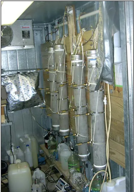
a local quarry. Figure 1 shows a photograph of the columns. All of the columns were operated in

a continuous flow mode at an average flow rate of 100 - 150 mL/d which is equivalent to a

groundwater velocity of ~3-4 cm/d. The influent to each column was amended with 15-20 mg/L

(1) Column 1 was operated as a biologically inhibited control. The influent to this column

was a 100 mg/L CaCl2 solution amended with HCl to reduce the pH to less than 3

inhibiting biological activity.

(2) Column 2 was designed to represent in situ conditions in a typical aquifer. During

packing, the field sand was amended with 250 mL of bioaugmentation culture enriched

from a site in Lumberton, NC. The influent to this column was a 100 mg/L CaCl2

solution.

(3) Column 3 was designed to represent in situ conditions in an aquifer with an active

methanogenic population. During packing, the sediment was amended with 250 mL of

the Lumberton bioaugmentation culture and 300 mL of anaerobic digester sludge. The

influent to this column was a 100 mg/L CaCl2 solution.

(4) Column 4 was operated to represent a soluble substrate bioremediation process. During

packing, the sediment was amended with 250 mL of the Lumberton bioaugmentation

culture and 300 mL of anaerobic digester sludge. The influent to this column was a 100

mg/L CaCl2 solution amended with 2000 mg/L sodium lactate and 1000 mg/L yeast

Figure 1: Photograph of 10 cm by 100 cm long continuous flow columns.

3.0 METHODS

3.1 Column Construction and Operation

Columns were packed with two inches of washed concrete sand at the bottom, followed by

clayey field sand, and finally topped off with another two inches of concrete sand. The column

packing took place under saturated conditions. Two to three inches of 100 mg/L deaired CaCl2

entrapment of air bubbles in the column and reduce oxygen exposure. Anaerobic digester sludge

was also added to columns 3 and 4 to evaluate the effects of a large methanogenic population on

reductive dechlorination.

Following packing, the columns were mounted in a constant temperature room maintained at 21o

C. The influent feed to each column was a 100 mg/L CaCl2 solution containing 2 – 4 mg/L of

dissolved oxygen. This influent was designed to represent aerobic groundwater flowing into an

edible oil barrier in the field. A 1-100 RPM Masterflex pump along with L/S 13 Masterflex

tubing was used to inject the influent. Gasbags were set up on the influent reservoirs and

effluent collection to reduce oxygen exposure and collect any volatile organic chemicals (VOCs)

released during the process.

Column operation started on September 16, 2002 (Day 0). Shortly after start up, all of the

columns were switched over to an influent solution containing 2000 mg/L lactate and 1000 mg/L

yeast extract for 18 days to establish anaerobic conditions. On day 17, 250 mL of Lumberton

bioaugmentation culture was injected through the column inlet to enhance anaerobic

biodegradation. On day 18, the attached pumps were then used to inject 500 mL of oil-water

emulsion. The 10% oil-water emulsion was prepared using a dairy homogenizer and included

the addition of polysorbate 80 and GMO. At the time of the emulsion injection 1000 mg/L yeast

extract was also added to the emulsion and the continuous lactate / yeast extract feed was

discontinued. The emulsion injection took place over a 5 hr time period and then the columns

were shut down to allow the oil to sorb to the sediment inside the column. Column operation

resumed on October 7, 2002 (Day 21) after a 3 day shut down period with the influent reservoirs

an influent concentration of 15 - 20 mg/L PCE. The influent for column 1 was also amended

with HCl to inhibit biological activity by lowering the pH. Column 4 influent was amended with

sodium lactate (2000 mg/L) and yeast extract (1000 mg/L). Columns 2, 3, and 4 received a

second bioaugmentation on day 123 by pumping 250 mL of Lumberton bioaugmentation into the

column inlet. The first and second bioaugmentation consisted of 250 mL of Lumberton culture.

Between day 252 and 268, a third bioaugmentation treatment consisting of feeding 400 mg/L

yeast extract for 16 days followed by addition of 375 mL of Lumberton bioaugmentation culture

for columns 2 and 3 by injecting through the inlet.

The influent and effluent from each column were regularly monitored for tetrachloroethene

(PCE), trichloroethene (TCE), dichloroethene (DCE) isomers, and vinyl chloride (VC), oxygen,

methane, ethene, ethane, pH, organic carbon, total carbon, chloride, nitrate, acetate, bromide, and

sulfate. Sampling frequency was weekly for the first 112 days and then every other week for the

remainder of the experiment. During sampling, the pumps were turned up to increase the flow

rate so that a 10 mL sample could be taken in 5 – 10 minutes. Syringes (10 mL) were attached to

inlet, outlet, and side sampling ports. The side sampling ports were sampled monthly after day

224. When only the outlet and inlet were sampled, a total of 40 mL per column (2 syringes from

each sample port) were collected. When all ports were sampled a total of 100 mL were

collected. Samples for VOC analysis were collected by injecting 2 mL of sample below the

water surface of a partially filled 40 mL vial and then topping the vial off with D.I. water. The

40 mL vial was then analyzed for chlorinated solvents (PCE, TCE, and DCE isomers) by

standard method 6200C (Purge and Trap Capillary Column Gas Chromatography). Another 5

mL was injected into a 10 mL vial and then the sample head space was analyzed by gas

TOC vial capped and stored in a refrigerator until analyzed for total organic carbon and

inorganic carbon. An Orion pH meter was used to measure the pH in a 5 mL sample from the

second syringe. Finally, dissolved oxygen was monitored using Chemetrics 0-1 mg/L D.O. test

kits. Samples (5 mL) were collected monthly, mixed with sodium bicarbonate eluent, allowed to

sit over night to precipitate iron, filtered, and analyzed by ion chromatography following

Standard Method 4110B for chloride, nitrate, acetate, bromide, and sulfate (Standard Methods

19th Edition, 1995).

3.2 Bromide Tracer Test

A bromide tracer test was performed to monitor breakthrough of a non-reactive tracer and

estimate the hydraulic retention time of each column. A syringe pump was spliced into the

influent of each column just before the inlet, allowing us to amend the influent solution with a

4000 mg/L bromide solution. Carefully recorded dates and volumes pumped, from both the

syringe pump and influent reservoir, allowed the influent concentration of bromide to be

calculated over the length of the test. During the bromide test, 5 mL samples were taken weekly

and analyzed for bromide by ion chromatography.

3.3 Gas Production

The composition of gas released from columns 2, 3, and 4 were determined by attaching a 1 mL

airtight glass syringe to gas sample ports located at the top of the columns. After collection, a

0.4 mL gas sample was injected into a GOW MAC gas chromatograph equipped with a thermal

composition was monitored on two separate occasions and similar results were found. Total gas

production was tracked by attaching a 5 mL syringe to the sample port and measuring the

volume of gas trapped since the previous sampling event.

3.4 Sediment Analysis

At the end of the project, the columns were shutdown and drained for 4 days. The sediment in

each column was then sampled for total carbon, PCE, TCE, DCE isomers, and VC by driving

two 1 inch diameter steel tubes through the length of the column. The tubes were then extracted,

the ends plugged with rubber stoppers, and stored in a cold room for 5 days. The tubes were

then cut into 10 cm segments, and each 10 cm sub-sample was analyzed for total carbon, PCE,

TCE, and DCE isomers.

3.5 Carbon Mass Balance Analysis

The amount of contaminant degraded can be determined from the effluent monitoring results and

the sediment samples collected at the end of the experiment. The theoretical carbon usage was

estimated based on the electron acceptor load entering each column. The amount of carbon

required for degradation of PCE and its daughter products was then assessed. The carbon

required for dechlorination of PCE to each daughter product was estimated from the equations

listed below. Total carbon usage was calculated by accounting for carbon used in oxygen

reduction and methanogenic fermentation. Other electron acceptors such as iron (III) were not

analyzed and were not included in the carbon balance. Sulfate, nitrate, and phosphate were not

present in significant amounts in the column influents or effluents. The following chemical

Electron Accepting Half Reactions

PCE Æ TCE C2Cl4 + H+ + 2 e-Æ C2Cl3H + Cl

-PCE Æ DCE C2Cl4 + 2 H+ + 4 e-Æ C2Cl2H2 + 2 Cl

-PCE Æ VC C2Cl4 + 3 H+ + 6 e-Æ C2ClH3 + 3 Cl

-PCE Æ Ethene C2Cl4 + 4 H+ + 8 e-ÆH4 + 4 Cl

-O2 ½ O2 + e- + H+Æ ½ H2O

CO2Æ CH4 CO2 + 8 H+ + 8 e-Æ CH4 + 2 H2O

Electron Donating Half Reactions

Soy Bean Oil C56H100O6 + 106 H2O Æ 56 CO2 + 312 H+ + 312 e-

Lactate C3H6O3 + 3 H2O Æ 3 CO2 + 12 H+ + 12 e

-Yeast Extract C5H7O2N + 8 H2O Æ ½ N2 + 5 CO2 + 23 H+ + 23 e-

The fraction of added carbon used for reductive dechlorination can then be calculated based on

the inorganic carbon that was collected in the effluent.

3.6 Permeability Measurements

Permeability measurements were taken at the beginning of the project and after 3, 6, 10, and 13

months of operation to evaluate the effects of each treatment on permeability loss. Flexible

tubing was connected to the inlet, outlet, and 3 sample ports. The flowrates in the columns were

then adjusted to generate a measurable head loss over the length of the column and the column

effluent was collected in a 25 mL graduated cylinder. At the end of the test, total flow, time, and

heads were recorded. This information along with the column dimensions allowed calculation of

K = Q/(AI)

where K is the permeability, Q is the flow rate, A is the cross sectional area, and (I) is the

hydraulic gradient.

4.0 EXPERIMENTAL RESULTS

4.1 Bromide Tracer Tests

Bromide tracer tests were conducted after 10 to 11 months of operation to estimate the effective

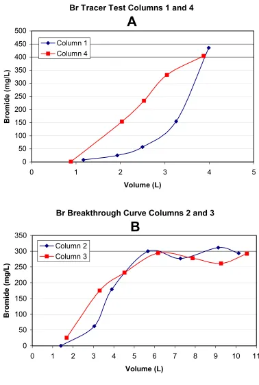
porosity and average hydraulic retention time (HRT) of each column. Figure 2 shows the

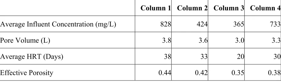
breakthrough curves for each test. Table 1 shows the average influent bromide concentration for

each column during the tracer tests. Once the effluent bromide concentration reaches 50% of the

average influent concentration, then the volume pumped through the column at that point is

considered to be one pore volume. Columns 1 and 4 had a five-week tracer test performed

where columns 2 and 3 had a seven-week tracer test performed. Although columns 1 and 4

tracer test lasted for a shorter duration, they were still ran long enough for the effluent

concentration to reach 50% of the average influent concentration and estimate a pore volume that

Br Tracer Test Columns 1 and 4

A

0 50 100 150 200 250 300 350 400 450 500

0 1 2 3 4 5

Volume (L)

Bromide (mg/L)

Column 1 Column 4

Br Breakthrough Curve Columns 2 and 3

B

0 50 100 150 200 250 300 350

0 1 2 3 4 5 6 7 8 9 10 11

Volume (L)

Bromide (mg/L)

Column 2 Column 3

Table 1: Pore volume and hydraulic retention times (HRT) estimated from bromide tracer tests.

Column 1 Column 2 Column 3 Column 4

Average Influent Concentration (mg/L) 828 424 365 733

Pore Volume (L) 3.8 3.6 3.0 3.3

Average HRT (Days) 38 33 20 30

Effective Porosity 0.44 0.42 0.35 0.38

The average hydraulic retention time (HRT) for each column was calculated based on the pore

volume and the average flow rate over the course of the project, not the duration of the tracer

test. Column 3 had the lowest effective porosity and shortest HRT of the four columns. Since

the same procedure was used to pack all of columns, the observed differences in effective

porosity between the columns are believed to be due to column operating conditions. Processes

that could lead to a lower effective porosity include biomass growth and accumulation of gas

bubbles. Column 3 which produced the most gas over the course of the project had the lowest

estimated porosity (0.35) and column 1 which had the lowest gas production had the highest

effective porosity (0.44). With increasing porosity, a general trend of increased average HRT

was observed. The longer the HRT the more contact time the contaminated water has with the

carbon source, which may result in more efficient degradation.

4.2 Column 1 – Low pH

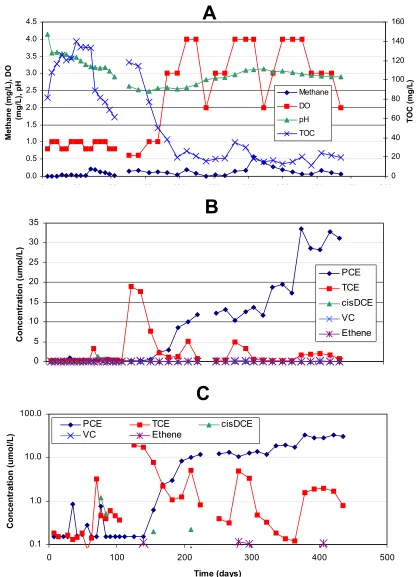
In Column 1 (Low pH), the effluent pH was initially around 4 and then dropped to below 3 as

the acid front migrated through the column (Figure 3). Around 200 days, the effluent dissolved

had been effectively suppressed. TOC concentrations averaged around 100 mg/L from shortly

after emulsion injection until around 150 days when concentrations declined to ~ 20 mg/L. At

around 100 days, significant levels of TCE began to appear in the column effluent, presumably

due to incomplete inhibition of biological activity by the low pH. However by 200 days, TCE

concentrations declined and PCE was, by far, the dominant ethene in the column effluent. PCE

concentrations in the column effluent have gradually increased with time, eventually reaching

half the average influent concentration of ~60 µmol /L. This indicates that the effective travel

time for PCE through Column 1 is approximately 400 days or approximately 10.5 times the

travel time for a non-reactive tracer (38 days). The longer travel time is attributed to PCE

sorption to residual oil in column one.

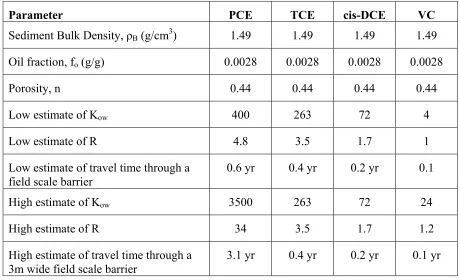
Chlorinated ethene partitioning between soybean oil and water can be approximated using the

octanol-water partition coefficient (Kow). Assuming instantaneous partitioning, retardation

factors for the different chlorinated ethenes were calculated using the equation

R = 1 + ρB fo Kow / n

and are presented in Table 2. The values presented in Table 2 are preliminary estimates. Best

estimate partition coefficients developed by calibrating the transport model to the observed

breakthrough will be presented in the modeling section. Porosity (n) was estimated from the

bromide tracer test. Sediment bulk density was estimated from the porosity and specific gravity

of quartz sand. The fraction oil (fo) in the sediment is based on the amount of sediment in

column 1 and the amount of soybean oil emulsion injected and is similar to oil retention values

observed in prior work (0.001 to 0.01 g/g) by Coulibaly and Borden (in press). Kow values were

Using the published range of Kow values, the effective retardation factor for PCE is expected to

vary between 7 and 38 while the observed retardation factor was 14 -19. The close match

between calculated and observed retardation factors for PCE in Column 1 suggests that

chlorinated ethene retardation in edible oil barriers can be reasonably approximated using a

linear partitioning approach.

Sorption of PCE to the entrapped oil will delay breakthrough in field scale edible oil barriers.

Table 1 also lists the estimated time for chlorinated ethene breakthrough in a typical field scale

barrier (3 m thick) with a groundwater flow velocity of 0.1 m/d (non-reactive travel time of 0.08

yr or 1 month). This breakthrough time is relevant because the HRT of the columns was

approximately one month. As can be seen in Table 2, PCE has the highest retardation factor and

could be retained in an edible oil barrier for up to 3 years. However, Kow values for the other

ethenes are lower and the maximum retention times for TCE, cis-DCE and VC are estimated to

be 0.4, 0.2 and 0.1 yr. This suggests that a significant amount of PCE may initially partition into

the soybean oil. However once an acclimated microbial community develops, PCE will be

converted to more soluble daughter products and these daughter products will rapidly migrate

through the column or barrier. The rapid breakthrough of TCE in Column 1 supports this

interpretation. High concentrations of TCE appeared in the Column 1 effluent approximately

112 days after the start of PCE injection. This is equivalent to a retardation factor of 3 for TCE,

Table 2: Estimated retardation factors for different chlorinated ethenes in Low pH - Column 1.

Parameter PCE TCE cis-DCE VC

Sediment Bulk Density, ρB (g/cm3) 1.49 1.49 1.49 1.49

Oil fraction, fo(g/g) 0.0028 0.0028 0.0028 0.0028

Porosity, n 0.44 0.44 0.44 0.44

Low estimate of Kow 400 263 72 4

Low estimate of R 4.8 3.5 1.7 1

Low estimate of travel time through a field scale barrier

0.6 yr 0.4 yr 0.2 yr 0.1

High estimate of Kow 3500 263 72 24

High estimate of R 34 3.5 1.7 1.2

High estimate of travel time through a 3m wide field scale barrier

Figure 3: Column 1 results: (A) ethene, methane, DO, pH and TOC (B) Variation in

effluent PCE, TCE, DCE, VC (C) Variation in effluent PCE, TCE, DCE, VC (log scale).

Low pH Column (1)

A

0 50 100 150 200 250 300 350 400 450 500

Time (Days)

Methane (mg/L), DO

(mg/L), pH 0 20 40 60 80 100 120 140 160 TOC (mg/L) Methane DO pH TOC

B

0 100 200 300 400 500

Time (days) Concentration (umol/L) PCE TCE cisDCE VC Ethene

C

0 100 200 300 400 500

Time (days)

Concentration (umol/L)

PCE TCE cisDCE

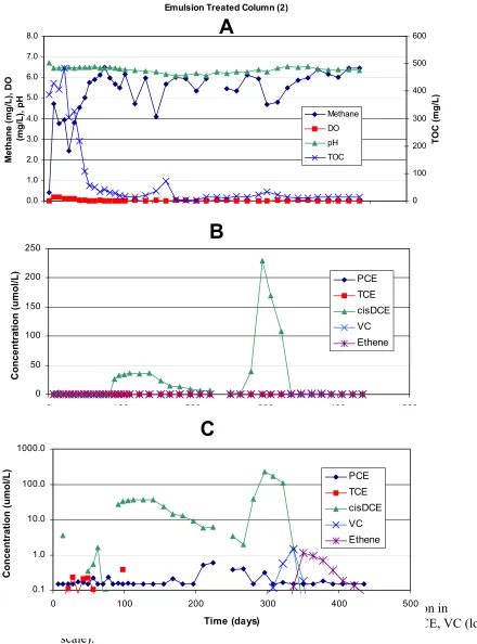
Figure 4: Column 2 results: (A) ethene, methane, DO, pH and TOC (B) Variation in

effluent PCE, TCE, DCE, VC (C) Variation in effluent PCE, TCE, DCE, VC (log scale).

Emulsion Treated Column (2)

A

0 50 100 150 200 250 300 350 400 450 500

Time (Days)

Methane (mg/L), DO

(m g/L), pH 0 100 200 300 400 500 600 TOC (m g/L) Methane DO pH TOC

B

0 100 200 300 400 500

Time (days) C oncent rat ion ( u mol/L) PCE TCE cisDCE VC Ethene

C

0 100 200 300 400 500

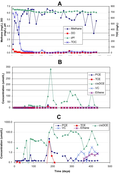
Figure 5: Column 3 results: (A) ethene, methane, DO, pH and TOC (B) Variation in

effluent PCE, TCE, DCE, VC (C) Variation in effluent PCE, TCE, DCE, VC (log scale).

Emulsion/Sludge Treated Column (3)

A

0 50 100 150 200 250 300 350 400 450 500

Time (Days)

Methane (mg/L), DO

(mg/L), pH 0 100 200 300 400 500 600 700 800 TOC (mg/L) Methane DO pH TOC

B

0 100 200 300 400 500

Time (days) Concent rat ion ( u mol/L) PCE TCE cisDCE VC Ethene

C

0 100 200 300 400 500

Time (days) Concent rat ion ( u mol/L)

PCE TCE cisDCE

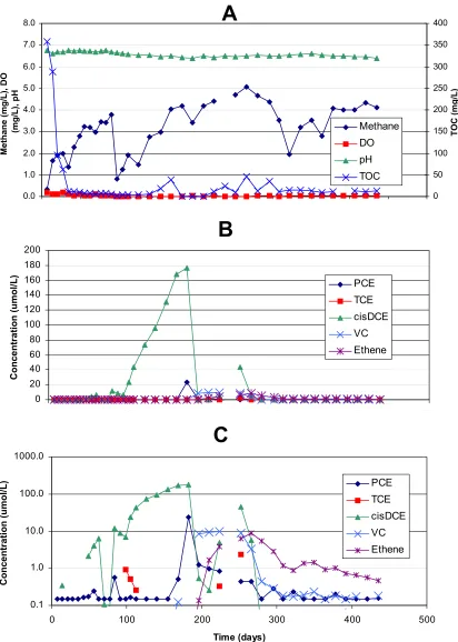
Figure 6: Column 4 results: (A) ethene, methane, DO, pH and TOC (B) Variation in

effluent PCE, TCE, DCE, VC (C) Variation in effluent PCE, TCE, DCE, VC (log scale).

Soluble Substrate Column (4)

A

0 50 100 150 200 250 300 350 400 450 500

Time (Days) Methane (mg/ L), DO (mg/L), pH 0 50 100 150 200 250 300 350 400 TOC (mg/L) Methane DO pH TOC

B

0 100 200 300 400 500

Time (days) C o n cen tratio n (u mo l/L ) PCE TCE cisDCE VC Ethene

C

0 100 200 300 400 500

4.3 Column 2 – Emulsion Treated

In Column 2 (emulsion treated column), the pH varied between 6 and 7 and DO remained below

0.1 mg/L indicating emulsion injection had generated condition appropriate for reductive

dechlorination (Figure 4). High concentrations of TOC broke though in the Column 2 effluent

shortly after emulsion injection. However TOC concentration then declined to 20-50 mg/L

concurrent with an increase in effluent methane concentrations. After day 100, methane

concentrations remained relatively constant varying between 4 and 6 mg/L. In addition, Column

2 released roughly 2 mL of gas bubbles each week. This gas is about 44% methane indicating

aqueous methane concentrations in the column effluent are slightly below equilibrium with the

gas released (0.44 * 24 mg/L, aqueous solubility of methane = 10 mg/L).

DCE broke through in Column 2 effluent at around 90 days and then remained constant at

concentrations comparable to the amount of PCE in the influent indicating relatively efficient

conversion of PCE to TCE to cis-DCE. However VC concentrations remained low (< .03

µmol/L) and there was no evidence of appreciable ethene production. Similar results were

obtained for Columns 3 and 4. In an attempt to stimulate complete reductive dechlorination of

cis-DCE to ethene, Columns 2, 3 and 4 each received an additional 250 mL of bioaugmentation

culture on day 123. This treatment was effective in stimulating complete reductive

dechlorination in Column 4 (lactate/yeast extract feed) but did not result in complete reductive

dechlorination in Column 2 (cis-DCE remained high; VC remained < .08 µmol/L, no significant

ethene production). On day 252, we began feeding a 400 mg/L solution of yeast extract to

Columns 2 and 3, followed by 375 mL of bioaugmentation culture on day 268. Immediately

The final treatment of yeast extract and bioaugmentation culture was successful in stimulating

complete dechlorination in Column 2. Around day 300, there was a dramatic increase in

cis-DCE in the Column 2 effluent followed by a rapid decline in cis-cis-DCE, temporary production of

VC and finally production of ethene. By day 400, TCE, cis-DCE and VC were below detection

with significant amounts of ethene present in the column effluent. However throughout this

period, low levels of PCE (up to 0.18 µmol/L) have been periodically detected in the effluent of

all the live columns (2, 3 and 4). However, up to 0.15 µmol/L (25 µg/L) PCE were occasionally

detected in laboratory blank samples, suggesting that the PCE detected in the column effluent

was likely due to carry over from the high concentration influent samples (60-120 µmol/L).

The high DCE concentration observed in the Column 2 effluent around day 300 was well in

excess of the influent PCE concentration (on a molar basis). The large pulse of cis-DCE

released is likely due to the biotransformation of PCE and/or TCE that had sorbed to the residual

soybean oil. The dramatic increase in microbial activity may be due to injection of yeast extract

solution from day 252 to 268 or due to bioaugmentation on day 268.

After 435 days of operation, Column 2 continued to reduce TCE, cis-DCE and VC to below

detection and remove over 99% of the influent PCE. Significant amounts of ethene were

detected in the column effluent. Columns 2, 3, and 4 had gas ethene production measured on

November 10, 2003 and the concentrations were 186 ppm, 759 ppm, and 332 ppm, respectively.

However these concentrations are orders of magnitude below the levels expected based on the

influent PCE loading. At this time, it is not clear what is happening to the ethene. Ethane

concentrations remain very low (< 0.04 µmol/L). Ethene has been detected in gas bubbles

cannot accurately estimate the mass of ethene released in the bubbles. Bradley (2003) proposed

several alternatives for the lack of ethene production during reductive dechlorination including:

(1) anaerobic oxidation of VC and DCE to yield CO2 or CO2 and CH4 (Bradley and Chapelle,

1996); (2) net oxidation with chloroethanol as intermediate (Vogel and McCarty, 1985); (3)

syntrophic oxidation with acetate as intermediate (Bradley and Chapelle, 1999, 2000); and (4)

syntrophic oxidation with ethene as intermediate (Bradley and Chapelle, 2002).

4.4 Column 3 – Emulsion and Digester Sludge Treated

In Column 3 (column treated with emulsion and anaerobic digester sludge), results were

generally similar to Column 2, which received emulsion only. In Column 3, the pH was also

between 6 and 7, with low DO (Figure 5). TOC concentrations where high immediately after

emulsion injection and then stabilized at around 10 mg/L once methane production increased.

Gas bubble production appears to have been slightly greater in this column, possibly due to

inoculation with anaerobic digester sludge. However aqueous methane concentrations are

similar and the gas produced is 30 – 45% methane at a rate of ~2.2 mL/wk.

DCE broke through in the Column 3 effluent at around 90 days and then reached a

quasi-steady-state. As in the emulsion only column, bioaugmentation of Column 3 at 123 days appears to

have stimulated conversion of some PCE or TCE trapped in the column but did not result in

significant VC or ethene production. However, injection of yeast extract and bioaugmentation

culture on day 268 appears to have stimulated some conversion of DCE to VC and ethene.

Around day 320, we observed significant levels of VC in the Column 3 effluent followed by

significant ethene production at day 400. While VC and ethene production have increased in

in fully degrading PCE. The less complete conversion of DCE in this column may be due to the

greater number of methanogens that could consume the bioavailable carbon before it can be

effectively used for reductive dechlorination. The shorter HRT for Column 3 (~ 20 days)

compared to Column 2 (~ 33 days) may also have contributed to the less efficient DCE

degradation.

4.5 Column 4 – Soluble Substrate

In Column 4 (fed lactate and yeast extract in column influent), results were generally similar to

Column 2 which received emulsion only. In Column 4, the pH was also between 6 and 7, with

low DO (Figure 6). TOC concentrations were high immediately after the start of soluble

substrate addition and then dropped to around 10 mg/L in the column effluent after day 35. The

soluble substrate column also released significant levels of dissolved methane (2- 5 mg/L).

However the gas bubble production was slightly lower, at ~1.4 mL/wk, than in Column 2 with a

somewhat lower methane fraction (20-25%).

DCE concentrations exceeded 10 µmol/L on day 84 and then steadily increased to over 606

µmol/L on day 184. The rapid increase in DCE after day 100, may be due to a second

bioaugmentation of Column 4 on day 123. Immediately following the decrease in DCE on day

184, we observed a temporary increase in VC followed by an increase in ethene. Column 4

provided very effective treatment up to day 450 with TCE, DCE and VC degraded to below the

analytical detection limit. As with the other columns, up to 0.18 µmol/L of PCE was

occasionally detected in the Column 4 effluent samples. These detections are believed to be due

to analytical carry over from the high levels of PCE in the column influent. Overall, the soluble

average HRT of 30 days, which could account for its more effective degradation when compared

to column 3.

4.6 Variations in Chloroethene Concentrations with Distance

Beginning on day 224, the side sampling ports were sampled monthly to measure the distribution

of each contaminant and associated indicator parameters. Sample ports A, B, and C are at

distances 0.25 m, 0.5 m, and 0.75 m respectively from the inlet of each column. In column 1,

only the movement of PCE through the column can be observed. However, each of the other

columns (2, 3, and 4) showed biodegradation of PCE to its daughter products (TCE, DCE, VC,

and ethene). By studying the migration of these daughter products through the columns, we can

gain a better understanding of the biotransformation processes occurring. The concentration

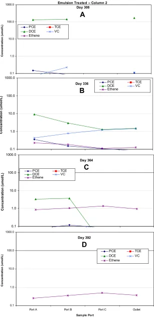
Figure 7: Chloroethene concentration profile over time in Emulsion Treated – Column 2: (A) Day 308 (B) Day 336 (C) Day 364 (D) Day 392.

Emulsion Treated -- Column 2 Day 308

A

Port A Port B Port C Outlet

Sam ple Port

Concent rat ion ( u mol/L) PCE TCE DCE VC Ethene Day 336

B

Port A Port B Port C Outlet Sample Port Co n cen trati o n (u mo l/ L ) PCE TCE DCE VC Ethene Day 364

C

Port A Port B Port C Outlet Sample Port Co n cen trati o n (u mo l/ L

) PCE_DCE TCE_VC Ethene Day 392

D

Port A Port B Port C Outlet

Sam ple Port

4.6.1 Emulsion Treated – Column 2

Figure 7 shows the spatial variation in the different ethenes in Column 2 following the third and

final bioaugmentation of the column on day 268. By day 308 the most prevalent compound in

all sample ports was DCE. This was expected since the average HRT is estimated at 33 days for

column 2. This means the bioaugmentation or yeast extract feed solution before

bioaugmentation was successful at stimulating reductive dechlorination to the point of DCE. By

day 336 DCE concentrations had declined by a factor of 10 in Port A and by a factor of 100 in

Port C. At this time, VC concentrations were increasing with distance along the length of the

column indicating gradual conversion of DCE to VC. On day 364, DCE was below detection in

the second half of the column, VC was below detection throughout the column, and ethene was

the dominant compound observed. All compounds other than ethene were non-detect by day

392. There was PCE in the effluent, but not in concentrations greater than the detection limit.

The general trend is for an initial production of DCE, followed by conversion of VC and ethene

once a large population of DCE degraders has developed. This suggests that for each daughter

product to be produced, a small acclimation period is needed for the microbes to adjust to the

changing contaminant environment. Once adaptation to the environment occurs, biodegradation

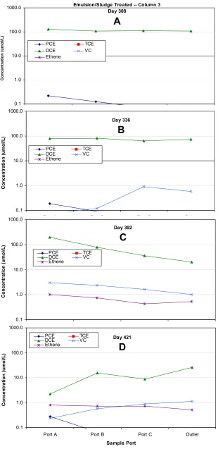
Figure 8: Chloroethene concentration profile over time in Emulsion/Sludge Treated – Column 3: (A) Day 308 (B) Day 336 (C) Day 392 (D) Day 421.

Emulsion/Sludge Treated -- Column 3 Day 308

A

Port A Port B Port C Outlet

Sample Port Co n cen trati o n (u mo l/ L ) PCE TCE DCE VC Ethene Day 336

B

Port A Port B Port C Outlet Sample Port Concentrati on (umol /L ) PCE TCE DCE VC Ethene Day 392

C

Port A Port B Port C Outlet Sample Port Concentrati on (umol /L ) PCE TCE DCE VC Ethene Day 421

D

4.6.2 Emulsion/Sludge Treated – Column 3

Figure 8 shows the spatial variation in the different ethenes in Column 3 following the third and

final bioaugmentation of the column on day 268. Similarly to column 2, addition of the

bioaugmentation culture and/or yeast extract solution was successful in stimulating DCE

production by day 308. By day 336, VC concentrations were beginning to increase with distance

from the inlet. By day 392, there was a significant decline in DCE concentrations over the

length of the column and production of significant amounts of VC. Significant levels of ethene

were also observed for the first time on day 392. By day 421, DCE concentrations were at the

columns lowest levels observed and VC concentrations were now increasing over the length of

the column. Ethene production on day 421 was sustained at a similar level to that on day 392

over the length of the column. The same trends observed in column 2 were also observed in

column 3, but at a somewhat slower rate. There was a period of DCE accumulation, followed by

VC production, then finally ethene production. However in column 2, DCE was degraded to

below detection by day 392 while significant levels of DCE were detected in column 3 past day

4251. The less effective conversion of DCE may be due to competition for available substrates

Figure 9: Chloroethene concentration profile over time in Soluble Substrate – Column 4: (A) Day 224 (B) Day 252 (C) Day 308.

Soluble Substrate -- Column 4 Day 224

A

Port A Port B Port C Outlet

Sample Port Concentration (umol/L) PCE TCE DCE VC Ethene Day 252

B

Port A Port B Port C Outlet

Sample Port Concentration (umolL) PCE TCE DCE VC Ethene Day 308

C

Port A Port B Port C Outlet

Sample Port

Concentration (umol/L)

PCE TCE

DCE VC

4.6.3 Soluble Substrate – Column 4

Figure 9 shows the spatial variation in the different ethenes in Column 4 following the second

bioaugmentation of this column on day 123. By day 224, DCE concentrations were already

declining with distance in column 4 with concurrent production of VC and ethene. By day 252,

DCE concentrations had declined further, with a slight decrease in VC and a slight increase in

ethene over the length of the column. On day 308, DCE was below detection in all sampling

ports, VC was low and ethene was the predominant compound in the column outlet. TCE, DCE

and VC were not observed in significant concentrations in any of the side sampling port in

column 4 on or after day 308. Degradation of PCE was more rapid and complete in column 4

than the other two live columns. The more efficient conversion of PCE in this column could be

due to: (a) the increased bioavailability of the soluble substrate (lactate) in the column feed, (2)

the presence of important nutrients in the yeast extract in the column feed, and/or (3) the longer

HRT of this column (30 days).

4.6.4 Summary of Results

By the completion of the project, all of the live columns (2, 3, and 4) were successful in reducing

PCE by over 99%. All columns also exhibited significant production of DCE before VC was

observed, and significant production of VC before production of ethene. By day 392, column 2

was only producing VC and ethene with ethene being the primary degradation product observed.

Column 3 took until day 392 to produce significant levels of ethene and by day 421 was still

producing substantial amounts of DCE. The lack of complete dechlorination in column 3 when

compared to column 2 may be due to methanogenic competition or the lower average HRT of

with lower levels of VC. The shorter acclimation period for complete dechlorination in Column

4 may be due to the greater bioavailability of the soluble substrate and/or trace nutrients in the

yeast extract feed.

Comparison of the side port monitoring results from columns 2 and 3 suggest that the observed

differences in contaminant degradation in these columns is not due to the shorter HRT of column

3. Most of the degradation occurred in the first 0.25 m of every column. Significant levels of

PCE and TCE were never observed in any of the side sampling ports. This suggests that

substrate availability may have limited contaminant biodegradation. Substrate could be limited

due to: (a) competition by high levels of methanogens; and/or (b) retention of most of the

organic substrate in the first 0.25 m of the column. In the carbon analysis section, results are

presented demonstrating that higher levels of organic substrate are present near the column inlet

with much lower levels present throughout the remainder of the column.

4.7 Final Chloroethene and Organic Carbon Distribution in Sediment

Sediment samples were collected after the completion of the PCE injection phase to determine

the final distribution of chloroethenes (PCE, TCE, and DCE) and carbon in the column sediment.

Two steel tubes were driven through the sediment. One tube was sectioned and analyzed for

chloroethenes while the second was analyzed for total carbon. In many cases, sediment samples

were not recovered from the full length of the column. As a consequence, the number and

location of samples analyzed for chloroethenes and carbon vary. For chloroethene analysis,

from 50 cm to 100 cm in column 2, from 80 to 100 cm in column 3, and from 30 to 100 cm in

column 4. For carbon analysis, samples were recovered in 10 cm increments from 20 to 90 cm

in column 1, and from 40 to 100 cm in columns 2, 3 and 4.

PCE, TCE and DCE concentrations versus distance from the inlet of each column are presented

in Figure 10. PCE and DCE concentrations in sediment are highest in the low pH column 1 with

much lower levels observed in the three live columns. The total mass of chloroethenes in each

column was estimated as the product of the arithmetic mean chloroethene concentration and the

mass of sediment in the column. In all cases, chloroethene concentrations were highest

immediately adjoining the column inlet. Where only a few sediment samples were analyzed, a

single high measurement could result in a biased estimate of the mass of chloroethenes recovered

in the sediment.

Total carbon concentrations versus distance from the inlet of each column are presented in

Figure 11. Significant amounts of organic carbon were distributed through out the length of the

three emulsion treated columns. However, there was also considerable variation between

adjacent samples indicating the emulsion was not uniformly distributed. With the exception of

one sample from the column 3 inlet, carbon concentrations were often significantly higher in low

pH column 1 than the two live emulsion columns (2 and 3) or soluble substrate column 4. The

higher levels of carbon remaining in column 1 is presumably due to the inhibition of biological

activity. The high carbon concentration in the column 3 inlet sample may have been due to

Figure 10: Chloroethene sampling over the length of each column: (A) Column 1 (B) Column 2 (C) Column 3 (D) Column 4.

Low pH -- Column 1 Sedim ent Sam pling Results

A

0 10 20 30 Distance from Inlet (cm)40 50 60 70 80 90 100

B

Em ulsion Treated -- Colum n 2 Sediment Sampling Results

B

0 20 40 60 80 100 120

Distance from Inlet (cm)

Chloroethene

Concentration (ug/g)

PCE TCE DCE

Emulsion/Sludge Treated -- Column 3 Sediment Sampling Results

C

0 20 40 60 80 100 120

Distance from Inlet (cm)

Chloroethene

Concentration (ug/g)

PCE TCE DCE

Soluble Substrate -- Column 4 Sediment Sampling Results

D

0 20 40 60 80 100 120

Distance from Inlet (cm)

Chloroethene

Concentration (ug/g)

Figure 11: Final carbon content versus distance for columns 1-4.

4.8 Chloroethene Mass Balance

An overall chloroethene mass balance was developed for each column by comparing the mass

injected with the cumulative mass in the effluent and mass sorbed to the sediment at the end of

the project. The cumulative mass of chloroethenes in the influent and effluent of each column

are shown in Figure 11. Cumulative mass was calculated as the sum of measured concentration

times the volume of water injected since the previous chemical analysis. During the

experimental period, there were four times when extremely high PCE concentrations were

detected in the column 1 influent samples. These very high concentrations are thought to have

occurred due to pumping non-aqueous phase PCE into the sample lines when the flow rates were

increased for sample collection. These very high concentrations are not believed to be

representative of what actually entered the column and were not included in the calculation of

cumulative mass entering the column. The observed concentrations may be high due to the

sampling method that requires the flow rate to be increased during the sample period. Overall

Carbon Sediment Samples with Distance

0.1 1 10 100

0 10 20 30 40 50 60 70 80 90 100

Distance from Inlet (cm)

Carbon (mg/g)

mass balance results for each column are presented in Table 3 including the amount of

Figure 12: Cumulative mass of ethenes in the influent and effluent: (A) Column 1 (B) Column 2 (C) Column 3 (D) Column 4.

Low pH -- Column 1

A

0 50 100 150 200 250 300 350 400 450 500

Time (days)

Total Ethenes

(umol)

Effluent Influent

Emulsion Treated Colum n 2

B

0 50 100 150 200 250 300 350 400 450 500

Tim e (days)

Total Ethenes

(umol)

Effluent Influent

Em ulsion/Sludge Treated Colum n 3

C

0 50 100 150 200 250 300 350 400 450 500

Time (days)

Total Ethenes

(umol)

Effluent Influent

Soluble Substrate Treated Column 4

D

0 50 100 150 200 250 300 350 400 450 500

Tim e (days)

Total Ethenes

(umol)

4.8.1 Column 1 – Low pH

As illustrated in Figure 12, substantially less chloroethene was discharged in the column 1

effluent than was introduced in the influent. However, most of this material was recovered as

PCE in sediment resulting in a final mass balance error of 18.6% ± 26%. The small residual

error may have been due to two leaks that occurred January 6 and May 12, 2003.

4.8.2 Column 2 – Emulsion Treated

In column 2, influent chloroethene mass was much greater than that of the effluent over the first

270 days. This difference indicates chloroethenes were being stored in the column and is

consistent with sorption of the more chlorinated species (PCE and TCE) to the entrapped

soybean oil. Around day 270, we see a rapid increase in effluent chloroethene mass due to high

concentration of DCE being released. However after day 350, total ethene levels in the effluent

remained low and influent mass remained greater than that in the effluent. By the end of the

experiment, the cumulative chloroethene mass in the influent was significantly greater than in

the effluent (Table 3). The total amount of chloroethenes recovered in the sediment at the end of

the experiment was less than 0.1% of the influent mass indicating that sorption to the sediment

was negligible.

In column 2, 36% of the influent mass was recovered in the column effluent with 64%

unaccounted for. The large mass balance error could be due to three factors: (1) errors in

estimation of the influent mass; (2) poor recovery of ethene in gas bubbles released from the

column; and (3) conversion of ethene to methane. As described above for column 1, excessively

high concentrations may have been due to the sample collection procedure and may not have

been representative of what was actually introduced into the column. However for column 2,

these high concentrations were retained in data set using for calculating influent mass. A portion

of the mass balance error could also be due to release of VC and ethene in gas bubbles. During

column operation, it was obvious that the gas collection procedure was not 100% effective and

some gas was being discharged in column effluent. However, based on the measured ethene

concentrations in the captured gas, this term is expected to make up only a small fraction of the

missing mass. Finally, ethene could potentially be oxidized to carbon dioxide or reduced to

methane as described by Bradley (2003).

4.8.3 Column 3 – Emulsion/Sludge Treated

Trends in cumulative influent and effluent chloroethenes in column 3 followed the same general

trends as in column 2. For the first 200 days, the influent mass of chloroethenes is much larger

than that of the effluent, which is consistent with sorption of PCE and TCE to the entrapped

soybean oil. Around day 200, there is a rapid increase in effluent chloroethene due to high

concentrations of DCE being released so by day 225, cumulative ethenes in the effluent are

approximately equal to those in the influent. From that point on column 3 continues to produce

chloroethene in the amount that are injected until significant VC and ethene production occur

around day 392. By the end of the experiment influent masses were greater than effluent

concentrations by 464 µmol (Table 3). Again, the difference is not due to sorption, but could be

4.8.4 Column 4 – Soluble Substrate

As shown in Figure 10, chloroethene mass recovery in the column 4 influent exceeded the

effluent until day 112. This indicates that significant sorption occurred in column 4, but not to

the extent in columns 2 and 3 which were treated with oil-water emulsions. Around day 112, the

effluent chloroethene mass recovery increased rapidly due to high concentrations of DCE being

released. By day 168, the total ethenes in the effluent are approximately equaled to that of the

influent. As occurred for columns 2 and 3, once significant levels of VC and ethene are

produced at around day 210, cumulative influent begins to exceed cumulative effluent.

Table 3: Summary of ethene mass balance results*.

In

(µmol)

Out (µmol)

Sediment (µmol)

Error (µmol)

Error (%)

Low pH - Column 1 1350 620 474 ± 345 256 ± 345 19 ± 26

Emulsion Treated -

Column 2 3380 1220 2.4 2158 64

Emulsion/Sludge

Treated - Column 3 4510 3910 136 464 10

Soluble Substrate -

Column 4 2010 1210 16 784 39

4.8.5 Summary of Chloroethene Mass Balance Results

In low pH column 1, sorption of PCE to the residual oil was significant. Sorption of PCE and/or

TCE was also important in the live emulsion treated columns. However once the columns were

effectively bioaugmented, the more highly chlorinated ethenes were converted to cis-DCE which

was rapidly discharged in the column effluent. These results are consistent with retardation

factors for PCE, TCE and cis-DCE estimated using a simple linear partition relationship and

published values of the octanol water partition coefficient.

In both columns 2 and 4, a significant fraction of the total ethenes introduced in the column

influent cannot be accounted for. These two columns were also very efficient in completely

dechlorinating PCE to gaseous endproducts. The poor mass balance observed in these two

columns may be due to poor recovery of ethene in gas bubbles released from each column or

further conversion of ethene to carbon dioxide or methane. While some portion of the ethene

mass was very likely released in the gas bubbles, it is unlikely that this can account for the entire

mass balance error.

4.9 Carbon Distribution in Column Effluent – Substrate Life

Figure 13 shows the cumulative mass of methane, organic, and inorganic carbon in aqueous

samples from the effluent of each column over the life of the project. Table 4 shows cumulative

carbon as methane, total organic carbon (TOC), and inorganic carbon (IC) as a mass and as a

percent of the organic carbon injected into each column as soybean oil emulsion or soluble

Figure 13: Effluent carbon distribution as methane, organic carbon, and inorganic carbon (A) Column 1 (B) Column 2 (C) Column 3 (D) Column 4.

Low pH -- Colum n 1

A

7 _{28 49 70 91}

112 155 196 238 280 322 364 406

Time (days)

Carbon (mg)

Organic Carbon

Inorganic Carbon

Emulsion Treated -- Column 2

B

7 _{21 35 49 63 77 91}

105 126 155 182 210 238 266 296 322 350 378 406 435

Tim e (days)

Carbon (mg)

M ethane Organic Carbon Inorganic Carbon

Em ulsion/Sludge Treated -- Column 3

C

7 _{21 35 49 63 77}

91 105 126 155 182 210 238 266 296 322 350 378 406 435

Time (days)

Carbon (mg)

M ethane Organic Carbon Inorganic Carbon

Soluble Substrate -- Colum n 4

D

7 _{21 35 49 63 77 91}

105 126 155 182 210 238 266 296 322 350 378 406 435

Time (days)

Carbon (mg)