University of Windsor University of Windsor
Scholarship at UWindsor
Scholarship at UWindsor
Electronic Theses and Dissertations Theses, Dissertations, and Major Papers
2011
Improving the Approximation Ratio of the Maximum Agreement
Improving the Approximation Ratio of the Maximum Agreement
Forest (MAF) on k trees and Estimating the Approximation Ratio
Forest (MAF) on k trees and Estimating the Approximation Ratio
of the Acyclic-MAF on k trees
of the Acyclic-MAF on k trees
Puspal Bhabak
University of Windsor
Follow this and additional works at: https://scholar.uwindsor.ca/etd
Recommended Citation Recommended Citation
Bhabak, Puspal, "Improving the Approximation Ratio of the Maximum Agreement Forest (MAF) on k trees and Estimating the Approximation Ratio of the Acyclic-MAF on k trees" (2011). Electronic Theses and Dissertations. 316.
https://scholar.uwindsor.ca/etd/316
IMPROVING THE APPROXIMATION RATIO OF THE MAXIMUM AGREEMENT FOREST(MAF) ON K TREES AND ESTIMATING THE
APPROXIMATION RATIO OF THE ACYCLIC-MAF ON K TREES
by
Puspal Bhabak
A Thesis
Submitted to the Faculty of Graduate Studies through Computer Science
in Partial Fulfillment of the Requirements for the Degree of Master of Science at the
University of Windsor
Windsor, Ontario, Canada
Improving the Approximation Ratio of the Maximum Agreement Forest(MAF) on k trees and Estimating the Approximation Ratio of the Acyclic-MAF on k trees
by
Puspal Bhabak
APPROVED BY:
Dr. Xiaobu Yuan School of Computer Science
Dr. Myron Hlynka
Department of Mathematics and Statistics
Dr. Asish Mukhopadhyay Advisor
School of Computer Science
Dr. Dan Wu Chair of Defence School of Computer Science
Author’s Declaration of Originality
I hereby certify that I am the sole author of this thesis and that no part of this thesis
has been published or submitted for publication.
I certify that, to the best of my knowledge, my thesis does not infringe upon
any-one’s copyright nor violate any proprietary rights and that any ideas, techniques,
quotations, or any other material from the work of other people included in my
the-sis, published or otherwise, are fully acknowledged in accordance with the standard
referencing practices. Furthermore, to the extent that I have included copyrighted
material that surpasses the bounds of fair dealing within the meaning of the Canada
Copyright Act, I certify that I have obtained a written permission from the copyright
owner(s) to include such material(s) in my thesis and have included copies of such
copyright clearances to my appendix.
I declare that this is a true copy of my thesis, including any final revisions, as approved
by my thesis committee and the Graduate Studies office, and that this thesis has not
Abstract
Molecular phylogenetics has long been a well-established field of scientific research
where the structure of the phylogenetic tree has been analysed to know about the
evolutionary process of the organism. In biology, leaf-labelled trees are widely used
to describe the evolutionary relationships. In this setting, the leaves of the tree
cor-respond to extant species, and the internal vertices represent the ancestral species.
However, for certain species, evolution is not completely tree-like. Reticulation events
such as horizontal gene transfer (HGT), hybridization and recombination play a
sig-nificant role in the evolution of the species. Suppose we have two phylogenetic trees
each of which is for a gene of the same set of species. Due to reticulate evolution
the two gene trees, though related, appear different. As a result, instead of the tree
like structure, a phylogenetic network is widely viewed as a most suitable tool to
represent reticulation. A phylogenetic network contains hybrid nodes for the species
evolved from two parents. The distance between two phylogenetic trees can be
com-puted with the help of a Maximum Agreement Forest (MAF) of those trees. The
fewer components in MAF, the greater is the similarity between the two trees. This
number of components in that agreement forest shows how many edges from each of
the two trees need to be cut so that the resulting forest agree after all forced edge
contractions. Recent research reveals that the MAF on k trees can be approximated
within a ratio of 8. We have given a better approximation ratio for the MAF on
k trees and also provide an approximation ratio for Maximum Acyclic Agreement
Dedication
to my
mother and father
Acknowledgements
I express my sincere gratitude to my advisor, Dr. Asish Mukhopadhyay for giving me
the opportunity to work under his supervision as well as for his guidance and support
in my research. I would like to thank Dr. Xiaobu Yuan for his valuable suggestions
and comments. I would also like to convey my sincere thanks to Dr. Myron Hlynka
for his advice and help.
I am thankful to my friends and colleagues in the Univeristy of Windsor for their
help and frequent assistance throughout my work and stay. Last but not the least, I
would like to thank my family for their love and confidence in my abilities that helped
Table of Contents
Page
Author’s Declaration of Originality . . . iii
Abstract . . . iv
Dedication . . . v
Acknowledgements . . . vi
List of Figures . . . ix
1 Introduction . . . 1
2 Basic Concepts . . . 5
2.1 Graph . . . 5
2.2 Binary Tree . . . 7
2.3 Phylogenetic network . . . 7
2.3.1 Properties of a hybrid network . . . 8
2.4 Agreement Forest . . . 9
2.5 Subtree Prune and Regraft(SPR) . . . 13
2.6 Tree Bisection and Reconnection(TBR) . . . 14
2.7 Nearest Neighbor Interchange(NNI) . . . 15
3 Literature review . . . 16
3.1 Hein et al. . . 16
3.2 Allen and Steel . . . 18
3.3 Baroni et al. . . 21
3.4.1 Fixed-Parameter Tractable . . . 23
3.5 Rodrigues et al. . . 23
3.6 Other work in this area . . . 24
3.7 Literature review with k(≥2) phylogeny trees . . . 25
4 Our Contribution . . . 32
4.1 Approximation Algorithms . . . 32
4.1.1 Terms and Definitions . . . 32
4.1.2 3-Approximation for MAF on k binary trees (rooted) . . . 35
4.1.3 2-approximation for MAAF on k rooted binary trees . . . 41
4.1.4 Heuristic . . . 45
4.2 Implementation . . . 46
5 Conclusion . . . 50
References . . . 52
List of Figures
1.1 Evolutionary Tree . . . 2
2.1 (a) Directed Graph (b) Undirected Graph . . . 6
2.2 Hybrid Network . . . 8
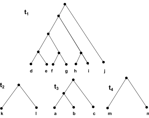
2.3 Three rooted phylogeny trees . . . 10
2.4 Agreement Forest of trees in Fig 2.3 . . . 11
2.5 A rooted treeT with leaf-set [a,b,c,d,e] , subtree T(L) and restriction subtreeT|L where L=[a,c,e] . . . 12
2.6 rSPR Operation . . . 13
2.7 TBR Operation . . . 14
2.8 This operation exchanges between B and C. Another NNI operation is possible between B and D . . . 15
3.1 Effect of a recombination. The genetic material (thick lines) that is now on one sequence was, just before the recombination, on two sequences, and the rest (thin lines) of the genetic material most likely does not have any descendent in the present sample. Recombination occurs at rp. [31] . . . 17
3.2 Two rooted binary phylogenetic trees reduced under Rule 1 . . . 19
3.3 Two rooted binary phylogenetic trees reduced under Rule 2 . . . 20
3.5 Topology of a tree with 3 leaves . . . 25
3.6 Conflicted Set of Triples. Any one leaf can be deleted from each tree to remove the conflict . . . 26
3.7 (i) A phylogeny treeT. The thick lines (rU) show the edges being cut to get the maximal size edge-disjoint set of triples and is stored in M1. (ii) A set of maximal size edge-disjoint set of triples have been cut from T according to Lemma 3.12 [18] . . . 29
3.8 If the maximal size edge-disjoint triple ((i,j),m) obtained from Fig 3.7 is a conflicted triple, sU is cut to remove the conflict and is added to M1. The leaf-set (g,h,k,l) will form the combination of triples in M2 . 29 3.9 (i) U1 = ((g,h),k) and U2 = (h,(k,l)) and w in this case is an edge. (ii) U1 = ((g,h),x) and U2 = (x,(k,l)) and w is a vertex. In either case remove the thick edges in case of incompatible triples in U1 and U2 . 30 3.10 i) 2 phylogeny trees T1 and T2. ii) Components in a forest which are topologically compatible in both T1 and T2. iii) For Separability check the components are in conflict with T1. So the graph has been formed with conflicted edges. The vertex cover of this graph will give d. So remove d from ii to get MAF. . . 31
4.1 Minimum incompatible triple is ab|c asab|c < xy|c . . . 33
4.2 Overlap Components [ [15], p:6] . . . 34
4.3 Central Lemma . . . 34
4.4 Layout of a minimal incompatible triple[ [15],p:5] . . . 36
4.5 MAF of T1 and T2 . . . 38
4.6 Directed Graph obtained from the MAF components in Figure 4.5. There is a cycle between t1 and t2. . . 40
4.7 MAAF obtained from the Directed Graph in Figure 5.6 . . . 41
4.9 Trees with leaf-set [A,B,C] and the MAF . . . 47
4.10 Trees with leaf-set [A,B,3,4,D,C] and the MAF . . . 48
Chapter 1
Introduction
Phylogenetic trees, or evolutionary trees are used in evolutionary biology to represent
the evolutionary history of biological entities such as present-day species or genes.
In a rooted phylogenetic tree, the leaves are uniquely labelled by the extant species,
while the internal nodes represent the ancestors. These are generally not labelled.
The universal common ancestor of all the species is represented as the root of the
tree. The out-degree of an internal node is the number of its children. The distance
between two nodes in an evolutionary tree represents evolutionary distance such as
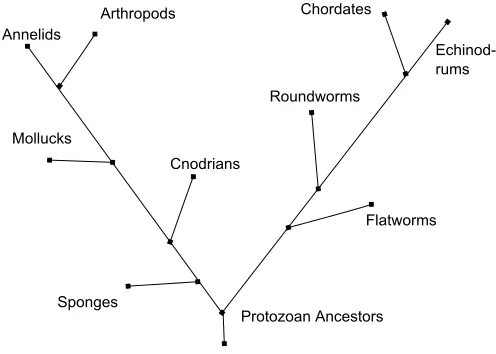
time or number of mutations. In figure 1.1 the evolutionary history of the Protozoan
Ancestors have been shown with the present-day species as the leaves of the tree.
This kind of representation is appropriate for many groups of species which include
the mammals. But it has been observed that not all groups follow the same
distri-bution of evolutionary patterns. Sometimes reticulation events come into play. This
type of evolution does not follow the tree like evolutionary process, rather the species
under reticulation events form a composite of genes derived from different ancestors.
The processes include hybridization, horizontal gene transfer and recombination.
re-Protozoan Ancestors Sponges Flatworms Roundworms Echinod-rums Chordates Cnodrians Mollucks Annelids Arthropods
Figure 1.1: Evolutionary Tree
search over the years that the evolutionary history of Eukaryotes contains
hybridiza-tion events that include certain groups of plants, birds and fish. Spontaneous
hy-bridization events have also been reported in the evolutionary history of some
mam-mals and even primates. Study on hybridization shows that at least 25% of plant
species and 10% of animal species, mostly the youngest species are involved in
hy-bridization events [43].
Several techniques have been devised to reconstruct phylogenetic trees from a given
set of species. Biologists are interested in determining the ’distance’ between two such
trees. Distance metrics such as NNI (Nearest Neighbor Interchange), SPR (Subtree
Prune and Regraft) and TBR (tree bisection and reconnection) have been proposed in
[53] for measuring the distance between the two phylogenetic trees. In an pioneering
paper Allen and Steel [2] proposed algorithms for estimating these distances. The
hybridization number and the rooted SPR (rSPR) distance have proven to be a very
useful tool in estimating the reticulation events that have occurred. Baroni et al. [5]
showed that rSPR distance provides a lower bound on the number of reticulation
Computing hybridisation number, rSPR and TBR distances have been shown to be
NP-hard problems [58]. Hence the interest in approximation algorithm and fixed
parameter tractable algorithm. Hein et al. [32] came up with the idea of Maximum
Agreement Forest(MAF) as a new tool to determine the distance between two
phy-logenies. They showed that a 3-approximation ratio algorithm exists for computing
the MAF for 2 trees is 3. They proposed a NP-hardness proof for computing SPR
distances. Allen and Steel [2] extended the NP-hardness idea of Hein et al. [32] to
prove that maximum agreement forest problem is NP-hard. In fact they rectified
cer-tain errors in the paper by Hein et al. [32] in their paper and showed that the TBR
distance between two trees is equal to the number of components in MAF. Rodrigues
et al. [53] with the help of certain instances showed that approximation ratio for the
size of MAF cannot be less than 4 which disproves the 3-approximation claim of Hein.
The approximation ratio later has been improved to 3 by Bordewich et al [15] for
the rSPR distance between two trees. Bordewich and Semple [16] showed that the
SPR distance between two rooted trees is also equal to the number of components in
MAF. Baroni et al. [5] introduced the concept of Maximum Acyclic Agreement
For-est(MAAF) and showed that the hybridisation number of two trees is one less than
the number of components in a MAAF. Chataigner [18] obtained an 8-approximation
ratio for the maximum agreement forest on k(≥2) trees.
In another approach to these problems, attempts have been made to find the Fixed
Parameter Tractable (FPT) algorithm when the distance between the two trees is
small. Allen and Steel [2] introduced certain tree reduction rules to obtain an FPT
algorithm for the TBR distance and the running time is O(k3k +p(n)) where k is
the distance between two trees and p(n) is a polynomial function of input size n.
Bordewich et al. [15] proposed an FPT algorithm for computing the rSPR distance
Our contributions in this thesis are the following:
A)A better approximation ratio in deriving the Maximum Agreement Forest on k
rooted phylogenetic trees
B)Estimate the approximation ratio of Maximum Acyclic Agreement Forest on k
trees.
C)An approximation algorithm for finding the rSPR distance between 2 trees, whose
approximation ratio we conjecture to be 2.
D)We have implemented the algorithm given in [15] on the 3-approximation ratio for
Chapter 2
Basic Concepts
This chapter introduces the basic concepts which have been used in this thesis.
2.1
Graph
This section deals with the prelimaries of graph theory. There are two kinds of graph:
directed and undirected.
A directed graph (or digraph) G=(V,E) consists of a set of verticesV and a set of
directed edges E such that for each edge e ∈ E there is a pair of vertices u,v ∈ V
connected at the two end-points ofe. Eacheis an ordered pair (u,v) so that the roles
of u and v are not interchangeable and we call u the tail of the edge and v the head.
In an undirected graph G=(V,E), the set of edges E consists of unordered pair
of vertices instead of having the ordered pairs. If an edge e ∈ E can be represented
by the pair of vertices (u,v) where u,v ∈ to the set of vertices V, then (v,u) also
represents the same edge e.
Many definitions for the directed and the undirected graphs are the same though there
1 2
3
4 5
1 2
3
4 5
a b
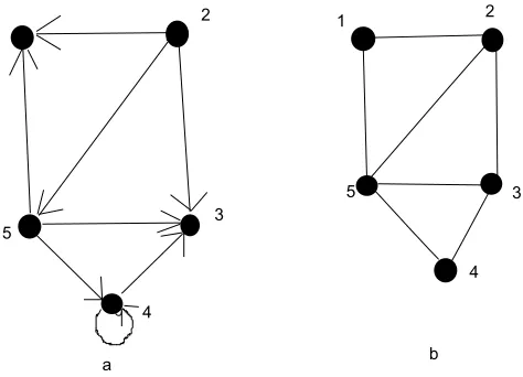
Figure 2.1: (a) Directed Graph (b) Undirected Graph
edge in a graph G= (V,E) we say that vertexv is adjacentto vertex u. When the
graph is undirected, the adjacency relation is symmetric. When the graph is directed
this symmetry is not always true. In figure 2.1(a) and (b) vertex 1 is adjacent to
vertex 2 since edge (2,1) belongs to both graphs. Vertex 2 is not adjacent to vertex
1 in figure 2.1(a) as the edge (1,2) does not belong to the graph.
The degree of a vertex in an undirected graph is determined by the number of
edges incident to it. In figure 2.1(b) the degree of the vertex 5 is 4. In a directed
graph, the out-degree of a vertex is the number of edges leaving the node and the
in-degree of the vertex is the number of edges entering it. So, in figure 2.1(a) the
out-degree of vertex 5 is 3 and the in-degree is 1.
A sequence of vertices <v0,v1,v2,...,vk> such that u=v0 and v=vk and (vi−1,vi) ∈
E, for i = 1,2, ..., k forms the path of length k from a vertex u to a vertex v in a
graph G= (V,E). The length of the path determines the number of edges in the
path. If v is reachable from u by a path p we write u ∼ v. In a directed graph a
path. In an undirected graph a path <v0,v1,v2,...,vk> forms a cycle if v0 = vk and
v0,v1,v2,...,vk are distinct. A graph with no cycle is called anacyclic graph. We say
an undirected graph is connected if every pair of vertices is connected by a path.
2.2
Binary Tree
A binary tree T is a data structure in which there are 3 disjoint set of nodes: a root
node, the subtree immediately to the left of root called left subtreeand the subtree
immediately to the right of the root known as the right subtree. Every internal
node in a binary tree other than the root is of degree 3. The nodes having degree 1
are called the leaves. The binary tree that contains no nodes is called a null tree. In
a binary tree the edges are directed away from the root. This gives an idea about the
parent-child relationship in a rooted binary tree [16]. Consider a node u in a rooted
tree T with root X. Suppose v be any node on the unique path from X to u in T.
Then v is known as the ancestor of u and u is the descendant of v. The length of
the path from the root X to a node u is the depth of u in T. The largest depth of
any node in T is the heightof T.
2.3
Phylogenetic network
In a phylogenetic tree The ancient ancestor is at the root of the tree. The leaf set
constitues the recent species and the internal nodes represent their ancestors. Due to
reticulation events, instead of the tree like structure, phylogenetic network is mostly
viewed as a tool to represent the reticulation which contains the hybrid nodes for
the species evolved from two parents [5]. Figure 2.2 shows the hybrid nodes cand f
a b c d e f g h i
Figure 2.2: Hybrid Network
2.3.1
Properties of a hybrid network
For a digraphD and a vertexv of D, we denote the in-degree and out-degree ofv by
d−(v) and d+(v), respectively. A hybrid phylogeny on the set of present-day species
X represented by the network H consisting of:
• a rooted acyclic digraph D in which the root has out-degree at least two and,
for all vertices v with d+(v) = 1, we have d−(v) ≥ 2
• the set of vertices of D with out-degree zero forms X.
It can be understood that, if|X| = 1, then the digraph consists of an isolated vertex
X. The setX corresponding to the set of present-day species is called the label set of
H and is denoted by L(H). Vertices of in-degree at least two are called
hybridiza-tion vertices. These vertices represent an exchange of genetic information between
hypothetical ancestors. For a hybrid H on X with root ρ the hybridization number
of H, denoted byh(H) is:
h(H) = X
v6=ρ
A rooted binary phylogenetic tree is a special type of hybrid phylogeny in which the
root has degree two and all other interior vertices have at least degree three. For two
rooted binary phylogenetic X-trees T and T0 [5], we get
h(T,T0) = min [h(H) : H is a hybrid on X that displaysT and T0]
2.4
Agreement Forest
LetT andT0be two rooted binary phylogenetic trees. We denote the set of leaf labels
of T as L(T), the set of branches as E(T). An agreement forest F for T and T0 is a
collection of rooted binary phylogenetic trees t1, t2,..., tn such that:
• for any tree ti, L(ti) ∈ L(T) and the union of L(ti) is equal to L(T)
• for eachti, the minimal subtree connecting the nodes inL(ti), denoted asS(ti),
is identical to ti when nodes with degree two of S(ti) are contracted
• for any two trees ti and tj, S(ti) and S(tj) are node disjoint
The size of a forest is the number of trees in the forest. An agreement forest is
ob-tained by cutting the same number of branches from bothT andT0 and after cleanup
gives rise to the same set of trees [60]. Agreement forests are an invaluable tool
for analyzing and understanding tree rearrangement operation. It can be observed
that the deleted edges are those which do not agree in T and T0 which suggest that
they represent the different paths of genetic inheritance i.e. hybridization events. An
agreement forest for T and T0 is a Maximum Agreement Forest (MAF) if, amongst
all agreement forests for T and T0, it has the smallest number of components.
The paper in [5] made an observation on the hybridization number problem which they
termed as Maximum Acyclic Agreement Forest (MAAF). This observation excludes
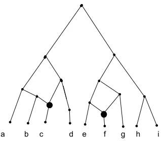
a b c k l
a b c
d e f g h i j
k l m n d e f g m n h i j
d e f g h i j
a b c
k l
m n
T1 T2 T3
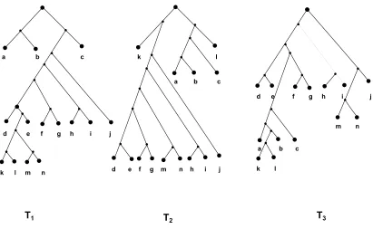
d e f g h i j
k l a b c m n
t
1t
2t
3t
4
Figure 2.4: Agreement Forest of trees in Fig 2.3
genetic information from its own descendants.
Let FA = [T1, T2, . . . , Tk] be an agreement forest for T and T0. Let GF be
the directed graph whose vertex set is FA and there is an edge from Ti toTj if i6=j
and either
• the root of T(L(Ti)) is an ancestor of the root of T(L(Tj)), or
• the root of T0(L(Ti)) is an ancestor of the root of T0(L(Tj)).
Since FA is an agreement forest, the roots of T(L(Ti)) and T(L(Tj)), and the roots
ofT0(L(Ti)) andT0(L(Tj)) are not the same. We say thatFAis an acyclic-agreement
forest if GF is acyclic. If FA contains the smallest number of components over all
acyclic-agreement forests forT and T0, we say thatFA is a Maximum Acyclic
Agree-ment Forest (MAAF) for T and T0. So, intuitively we can say a forest is a MAAF if
a b c d e
T
a c e
T(L) L = {a,c,e}
a c e
T|L
Figure 2.5: A rooted tree T with leaf-set [a,b,c,d,e] , subtree T(L) and restriction
subtree T|L where L=[a,c,e]
In [5], Baroni et al. established and proved a fundamental relation between
hy-bridization number and MAAF by the following theorem.
The hybridization number of T and T0 is equal to the size of the MAAF for T and T0
minus one.
Hence, it is essential to estimate the MAAF of two phylogenetic trees in order to
know their hybridization number.
Definition 1. For a tree T and a subset L of the leaf-set of T, the subtree
in-duced by L, noted as T(L) is the tree defined as the smallest connected subgraph of
T containing L. The restriction of T to L denoted as T|L is obtained from T(L) by
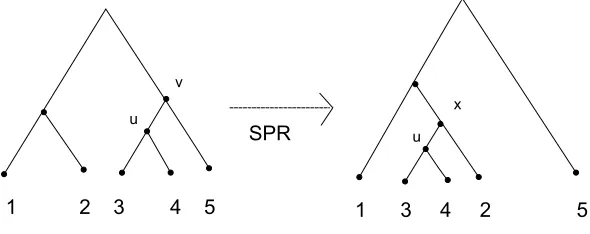
1 2 3 4 5
v
u x
u
1 3 4 2 5 SPR
Figure 2.6: rSPR Operation
2.5
Subtree Prune and Regraft(SPR)
Another very important tool used to understand reticulate evolution is the subtree
prune and regraft (SPR) [15] approach which measures the distance between
phylo-genies. If there are two phylogenies having the similar set of species but reticulation
has occurred, then this inconsistency in the parent-child relationship between the two
trees can be explained by the subtree prune and regraft operation. Given a subtree
T, an SPR operation on a particular edge e = [u,v] in T divides the tree into two
subtreesTu and Tv having the vertices uand v respectively. In order to reattach one
subtree say Tu to a different edge in Tv it bisects another edge f = [u0,v0] of Tv at
x and adds an edge between u and x. Finally the degree-two vertex v is contracted.
This kind of operation can take place in both rooted and unrooted trees. SPR(T,T0)
measures the minimum SPR operations required to transform T to T0. Figure 2.6
1 2 3 4 5
v
u
1 3 4 2 5
1 2 5 3 4
x
v
y u
x y
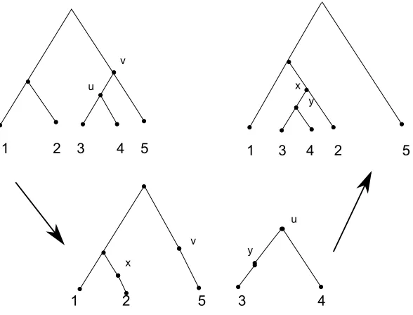
Figure 2.7: TBR Operation
2.6
Tree Bisection and Reconnection(TBR)
This method used to measure the distance between phylogenies works similar to SPR
with a slight modification. Given a subtreeT, a TBR operation on a particular edge
e = [u,v] in T divides the tree into two subtrees Tu and Tv having the vertices u
and v respectively. In order to reattach one subtree say Tu to a different edge in
Tv it bisects an edge in each of Tu and Tv atx and y respectively and adds an edge
betweenxandy. Finally the degree-two verticesuandv are contracted [2]. This kind
of operation can take place in both rooted and unrooted trees. TBR(T,T0) measures
the minimum TBR operations required to transform T to T0. Figure 2.7 illustrates
A
B
C
D
u v
A
D
u v
C
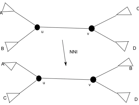
B NNI
Figure 2.8: This operation exchanges between B and C. Another NNI operation is possible between B and D
2.7
Nearest Neighbor Interchange(NNI)
This metric for measuring the distance between phylogenies has been introduced
in [44] and [52]. In a NNI operation two subtrees which are separated by an internal
edge can be swaped. By an internal edge (u, v) in a tree we mean neither u nor v
is a leaf of the tree. The operation only operates on the internal edge. NNI(T,T0)
measures the minimum NNI operations required to transform T to T0 [20]. Figure
2.8 explains an NNI operation.
Each of the metrics, TBR distance, rSPR distance and hybridization number, have
been proved to be one less than the number of components in a Maximum Agreement
Chapter 3
Literature review
In this chapter we deal with the work done about the computational aspect on
phy-logeny trees. To the best knowledge of our survey in this area, Hein (1993) [31] started
this area with his heuristic method to reconstruct the history of sequences subject
to recombination. Sections 3.1 to 3.6 contain the survey of the work done with 2
phylogeny trees. In Section 3.7 we have discussed about the work done on k trees.
3.1
Hein et al.
Hein (1993) [31] in his paper presented a heuristic method to reconstruct the history
of sequences due to recombination. In his paper he has shown the pictorial
represen-tation of the recombination. It has been proposed in his paper that the evolution of
a sequence with k recombinations could be described by k recombination points and
k+ 1 trees describing the evolution of thek+ 1 intervals, where two neighboring trees
were either identical or differed by the transfer of one subtree within the whole tree.
The heuristic algorithm in [31] generates trees that are one recombination away from
a given tree. The algorithm recursively visits all possible subtrees by visiting all
in-ternal edges. For every edge visited there will be a left and a right subtree. The left
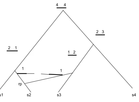
s1 s2 s3 s4 rp
1 1
2 1
1 2
2 3 4 4
Figure 3.1: Effect of a recombination. The genetic material (thick lines) that is now on one sequence was, just before the recombination, on two sequences, and the rest (thin lines) of the genetic material most likely does not have any descendent in the present sample. Recombination occurs at rp. [31]
one recombination away from a given tree.
Hein et al.(1996) extended their work [32] to show that computing the subtree-transfer
distance between two evolutionary trees is NP-hard and gave an approximation
al-gorithm with performance ratio 3. The idea of Maximum Agreement Forest came
from their work but it was not clearly defined. The basic idea behind this algorithm
is to select a pair of sibling leaves (a, b) in the first tree T1 at a time. If the pair a
and b are siblings in the second treeT2, this pair is replaced with a new leaf labeled
(a, b) in both the trees. Otherwise, T2 is being cut until a and b become siblings or
separated. This has been handled by considering 5 different cases. They have proved
a very useful relation which is stated below:
Lemma 3.1 [32]: The size of a MAF of T1 and T2 is one more than their
3.2
Allen and Steel
Allen and Steel (2000) in their paper discusses the problem of determining how far
apart two reconstructed trees are from each other or from the true historical tree. The
metrics they investigated are Nearest Neighbour Interchange (NNI), Subtree Prune
and Regraft (SPR), and Tree Bisection and Reconnection (TBR).
The main contributions in their paper are:
Lemma 3.2 [2]: 1. NNI ⊆ SPR ⊆ TBR
2.If dθ(T1, T2) denotes the minimum number of θ operations required to transform
the unrooted binary trees T1 to T2 where θ ∈ [NNI, SPR, TBR] then
a. dT BR(T1, T2) ≤ dSP R(T1, T2) ≤ dN N I(T1, T2)
b. dSP R(T1, T2) ≤ 2 * dT BR(T1, T2)
Allen and Steel [2] rectified certain errors in Lemma 3.1 [32] and showed that this
Lemma does not hold true for unrooted trees and also for SPR transformations. But
it is true if TBR operations are taken into consideration. This fact is established in
the following lemma:
Lemma 3.3 [2]: Suppose we have two unrooted binary treesT,T0 with L(T) = L(T0). Then,
1. dT BR(T,T0) = m(T,T0)
2. dSP R(T,T0) ≥ m(T,T0) where m(T,T0) is the size of MAF(T,T0) - 1.
They introduced the concept of Fixed Parameter Tractable (FPT) in measuring the
distance between two trees and showed the running time for the TBR distance is
A T1
a T'1
T2
T'2
A
a
Figure 3.2: Two rooted binary phylogenetic trees reduced under Rule 1
function of input size n. In order to establish the FPT, they have kernalised the
problem, that is the size of the problem has been reduced in such a way so that the
answer to the reduced problem is same as that of the original problem. In order to
kernalize the size of the problem in measuring the SPR or TBR distance they
pro-posed to apply the following 2 rules repeatedly:
Rule 1: Replace any pendant subtree that occurs identically in both trees by a
single leaf with a new label.
Rule 2: Replace any chain of pendant subtrees that occurs identically in both trees
by three new leaves with new labels correctly orientated to preserve the direction of
A1 A2
A3 An
a b
c
T1
T' 1
An
A3 A2
A1
c b
a
T2
T' 2
Figure 3.3: Two rooted binary phylogenetic trees reduced under Rule 2
1 2 3 4 1 3 2 4
T1 T2
1 2 3 4 H
Figure 3.4: T1, T2 are two phylogenetic trees and H is the hybrid network of T1
3.3
Baroni et al.
Baroni et al.(2004) in their paper [6] analyzed Acyclic directed graphs (ADGs) which
have been viewed as more appropriate for representing certain evolutionary
relation-ships, and have developed a framework for the analysis of these graphs which are
termed as hybrid phylogenies. Their work determines a hybrid phylogeny from a
given set of phylogenetic trees which shows the smallest number of hybridisation
events. They derived a very important equation:
h(H) ≥ |V| - 2|χ| + 1
where h(H) is the hybridisation number,V is the vertex set and χ is the leaf-set.
Baroni et al.(2005) in their paper [5] gave a very clear definition about the
con-cept of Maximum Agreement Forest and the conditions which need to be satisfied in
order to get a MAF between two rooted binary phylogenetic trees. The paper also
introduced for the first time the idea of Maximum Acyclic Agreement Forest(MAAF)
and the way to determine the MAAF from MAF by removing the cycles. The most
significant contribution of this paper has been the mathematical derivation of the
following Theorem:
Theorem 3.4 [5]: Let T and T0 be two rooted binary phylogenetic trees. Then h(T,T0) = mg(T,T0),
where h(T,T0) is the hybridisation number and mg(T,T0) is the number of components
in MAAF(T,T0) minus one
The paper also established the upper and lower bounds for h(T,T0).
χ-trees. Then for all n ≥ 2, drSP R(T,T0) ≤ h(T,T0) ≤ n-2
3.4
Bordewich et al.
Bordewich et al.(2004) [16] has showed that computing the rooted subtree prune and
regraft distance between two rooted binary phylogenetic trees on the same label set
is NP-hard. In this paper they have established the relation between rSPR distance
and the MAF of two rooted binary phylogenetic trees.
Theorem 3.6 [16]: Let T and T0 be two rooted binary phylogenetic trees. Then drSP R(T,T0) = m(T,T0), where m(T,T0) is the size of MAF(T,T0) - 1
Using the two reduction rules as mentioned in [2] they have shown that computing
the rSPR distance between two rooted binary phylogenetic trees is fixed parameter
tractable considering the rSPR distance itself to be the parameter.
Proposition 3.7 [16]: Let T1 and T2 be two rooted binary phylogenetic trees. LetT01
and T02 be two rooted binary phylogenetic trees obtained from T1 and T2 respectively
by applying either Rule 1 or Rule 2. Then dSP R(T1, T2) = dSP R(T01, T02)
Lemma 3.8 [16]: Let T1 and T2 be two rooted binary phylogenetic χ-trees. Let
T01 and T02 be two rooted binary phylogenetic χ0-trees obtained from T1 and T2
re-spectively by applying either Rule 1 or Rule 2 repeatedly until no further reduction is possible. Then |χ0| ≤ 28dSP R(T1, T2)
Bordewich and Semple(2007) in their work [17] has shown that computing the
two reduction rules.
Lemma 3.9 [17]: Let T and T0 be two rooted binary phylogenetic χ-trees and let P be an empty collection of 2-element subsets of χ. Let S andS0 be two weighted phy-logenetic χ0-trees obtained from T and T0, respectively, by repeatedly applying Rules 1 and 2 until no further reduction is possible. Then |χ0| < 14h(T, T0)
Bordewich et al.(2007) derived a 3-approximation algorithm SPR-APPROX(T,T0)
for the subtree distance between phylogenies [15]
Theorem 3.10 [15]: Let T and T0 be two rooted binary phylogenetic X-trees and let |X| = n. Let (F,k) be the output of SPR-APPROX(T,T0). Then F is an agree-ment forest for T and T0 and k is a 3-approximation for drSP R(T,T0).
Theorem 3.10 is the main contribution of this paper.
3.4.1
Fixed-Parameter Tractable
The running time of the SPR-EXACT algorithm [15] to compute the fixed-parameter
on the rSPR distance has been improved to O(4kk4+n3) by using the kernelisation
of Bordewich and Semple [17]. As a result upon the completion of the kernelisation
the resulting two rooted binary phylogenetic trees T and T0 have leaf sets of size at
most 28drSP R(T, T0).
3.5
Rodrigues et al.
Rodrigues et al. [53] with the help of certain instances showed that approximation
ratio for the size of MAF cannot be less than 4 which disapproves the 3-approximation
algorithms for this problem.
3.6
Other work in this area
Hallett and McCartin(2006) in their paper [29] have given an efficient fixed-parameter
tractable (FPT) algorithm for the MAF problem for 2 unrooted trees, and have
claimed to make a significant improve on an FPT algorithm given in [2]. The
run-ning time has been improved from O(k3k + p(|L|) in [2] to O(4k.k5)+ p(|L|) where k
bounds the size of the agreement forest and L is the leaf label set.
Hickey et al.(2008) in their paper [34] have shown that the unrooted SPR distance
computation is NP-Hard and has verified which techniques from related work can
and cannot be applied. They have also presented an efficient heuristic algorithm for
this problem and experimented with it on a variety of synthetic datasets. They have
claimed to provide an algorithm that computes the exact SPR distance between
un-rooted tree. With the help of the reduction rules to give a FPT approach to this
problem the running time of their algorithm isO(nk+2).
Bonet and St.John (2010) in [13] have shown that subtree prune and regraft (uSPR)
distance on unrooted trees is fixed parameter tractable with respect to the distance.
They have claimed to make progress on a conjecture of Steel [2] on the preservation of
uSPR distance under chain reduction and have improved on lower bounds of Hickey
et al. [34].
Wu and Wang (2010) in [60] have presented a new practical method to compute
the exact hybridization number. Their approach is based on an integer linear
a b c
b c a
c a b
Figure 3.5: Topology of a tree with 3 leaves
3.7
Literature review with
k
(
≥
2) phylogeny trees
In this chapter we describe Chataigner’s approximation ratio for finding the MAF on
k rooted binary trees. As per our knowledge this is the only work done in the field
regarding the computational aspect on k trees [18].
Definition 1. Given 3 leaves a,b,c of the tree T, we call the subtree connecting
the three leaves in T the triple in T. The topology of a tree T is the unique binary
tree of which T is a subdivision. For example, if T is a tree with three leaves [a, b,
c], there are 3 possible topologies for T, which can be represented as ((a, b), c), ((b,
c), a) and ((a, c), b) respectively. See figure 3.5.
Definition 2. For a tree T and a subset L of L(T), the subtree induced by L,
noted T|L is the tree defined as the smallest connected subgraph of T containing L.
Given two trees A and B, a triple of leaves U = [a, b, c] is a conflict if the induced
subtreesA|U and B|U have different topologies. See Figure 3.6.
a b c a c b
Figure 3.6: Conflicted Set of Triples. Any one leaf can be deleted from each tree to remove the conflict
iff they do not have any conflict.
A forest F can be obtained from a given set of trees Ti having similar species by
the partition of the leaves (species being represented by leaves) L such that:
Ptopo: for each j∈[1..m], the subtrees Ti|Lj induced by Lj have the same topology,
and the partition induces a subforest on T1
Psep: for each i∈[1..k], the subtrees Ti|Lj are vertex-disjoint.
Ptopo takes care of the first 2 rules for the formation of agreement forest described in
section 2.4 and Psep suffices the 3rd rule in the agreement forest formation.
Ptopo Check
be found in polynomial time.
This collection of the maximal size of edge-disjoint subtrees can also be found through
Integer Linear Programming(ILP) and this gives the lower bound in detrmining the
approximation ratio of MAF on k trees in their paper.
We start with a set of triples < in L(T) and another set M which contains the
minimal set of conflict edges. A decision variable de has been defined to take the
value based on the edges present inM. The main object is to have minimum number
of edges inM so as to maximise the agreement forest.
min X
e∈E(T)
de, E(T) is the edge-set of T
a ∈U, X
e:e∈T|a
de ≥ 1, U∈ <
de ∈ {0; 1}, de = 1 if e ∈ M
Relaxing this ILP to a linear program and taking the dual the maximal flow in the
tree has been determined.
max X
a∈U)
fa
e ∈E(T), X
a:e∈T|a
fa ≤ 1
fi ≥ 0, fi is the flow
This linear program can be strengthened to an integer program where fi ∈ [0; 1].
Max integral flow ≤ max fractional flow = min fractional multi-cut ≤ min multi-cut
Max integral flow (Υ) becomes the lower bound of the solution where Υ ⊂ <
Lemma 3.12 suggests it is possible to cut a collection of maximal size of edge-disjoint
set of triples Υ. For each triple U = [a, b, c], with topology ((a, b), c) for T|U , let rU
denote the root of T|U, defined as lca(a, c) [lca means lowest common ancestor] inT,
and sU denote the node lca(a, b). Let M1 be the set of edges entering the nodes rU
and sU , for all triples U∈Υ. Let us consider the set of triples <1∈U such that T|U
does not contain an edge in M1. Let the set beM2 which contains at least one edge
from<1. It has been illustrated in figures 3.7 and 3.8.
Lemma 3.13 [18]a triple U∈<1 sharing nodes with a triple V∈Υsatisfies r(T|U) ∈
T|V where r(T|U) is the root of T|U
Lemma 3.14 [18] a triple U∈<1 shares nodes with at most one triple from Υ.
For each triple V = [a, b, c]∈Υ, let <V be the set of triples in U∈<1 such that
T|U shares nodes with T|V = ((a, b), c). According to Lemma 3.13 [18] and Lemma
3.14 [18], <1 is a disjoint union of the UV.
Lemma 3.15 [18] if U1,U2∈<V are such that T|U1∩T|U2 6= φ, then there exists
w∈T|V such that w ∈ T|U1∩T|U2.
We now split <V in two parts. Let d be the parent of sV and let W1 be the set
a b c
i j g h k l m
d e f
ru
ru
(i) (ii)
a b c
i j m
d e f
Figure 3.7: (i) A phylogeny tree T. The thick lines (rU) show the edges being cut
to get the maximal size edge-disjoint set of triples and is stored in M1. (ii) A set of maximal size edge-disjoint set of triples have been cut from
T according to Lemma 3.12 [18]
i j g h k l m
su
Figure 3.8: If the maximal size edge-disjoint triple ((i,j),m) obtained from Fig 3.7
is a conflicted triple, sU is cut to remove the conflict and is added to
c g h k l b a c g h x k l b a
w w
(i) (ii)
Figure 3.9: (i) U1 = ((g,h),k) and U2 = (h,(k,l)) and w in this case is an edge. (ii) U1 = ((g,h),x) and U2 = (x,(k,l)) and w is a vertex. In either case remove the thick edges in case of incompatible triples in U1 and U2
common with T|d,c. By construction, <V =W1 ∪ W2
Lemma 3.16 [18] Either W1 = φ or W2 = φ
From Lemma 3.15 [18] and Lemma 3.16 [18] we can say any 2 triples in either W1
or W2 have some elements w common with T|V. w can be either an edge in which
M2 contains that edge or it can be a node in which 2 edges need to be added toM2.
This is illustrated in Fig 3.9. So altogether the size is bounded by 4|Υ|. Hence if the
size of the MAF is m∗, this step produces at most 4m∗ connected components. The
cut is being made on a single tree sayT1.
Psep Check
For every edge a of the forest F thus obtained from the above step, we consider
1 2 3 4 5 6 7 4 5 6 1 2 3 7
T1 T2
i)
1 2 3 7 4 5 6 a b d e f ii) iii) d a b
Figure 3.10: i) 2 phylogeny trees T1 and T2. ii) Components in a forest which are topologically compatible in both T1 and T2. iii) For Separability check the components are in conflict with T1. So the graph has been formed with conflicted edges. The vertex cover of this graph will give d. So remove d from ii to get MAF.
Ti under consideration. Chataigner’s algorithm proceeds as follows:
• build the graph G whose nodes represent the edges of F and an edge (a, b) ∈
E(G) represent a collision, i.e., some i such that Pi(a)∩Pi(b) 6=φ.
• compute a vertex cover ofG.
• for each node a of the vertex cover, remove one edge from P1(a).
This has been illustrated in figure 3.10.
If we consider the minimum number of components required to ensurePsepis bounded
by m∗ then at most 2m∗ edges can be removed. Since the minimum vertex cover
problem can be approximated within a ratio 2, the step needs at most 4m∗ edges
to be removed. Hence, altogether 8m∗ edges are removed from T1 which gives an
Chapter 4
Our Contribution
4.1
Approximation Algorithms
The work in this chapter has been motivated by the work of Bordewich et al. [15]. To
begin with, we introduce some terms and definitions that are relevant to our work.
4.1.1
Terms and Definitions
1. Partial Order [15]: In mathematics, Partial order means the concept of ordering
the arrangement of certain pairs of elements in a set. In the forestF of a phylogenetic
tree T, for two elements x and y (elements are the union of the vertex and edge sets
of F) which are in the same component of F, we write x < y if x 6=y and y lies on
the path from x to the root of this component.
2. Incompatible triple [15]: A triple is a rooted binary phylogenetic tree which
has 3 leaves. A triple with leaf set{a, b, c} can be denoted by ab|cif cdoes not lie on
the path from a tob in that triple.
If T and T0 be two rooted binary phylogenetic trees and {a, b, c} be the leaf set in
bothT and T0, then we say the tripleab|cis an incompatible triple of T with respect
a b x y c rabc
rab
Figure 4.1: Minimum incompatible triple is ab|cas ab|c < xy|c
the incompatible triple. Letab|cbe an incompatible triple inT and letrabc represent
the most recent common ancestor of a and c inT and rab represent the most recent
common ancestor ofaand binT. We sayab|c < xy|z if either i) rxyz lies on the path
fromrabc to the root ofT or ii)rxy is on the path fromrab to the root ofT if rabc and
rxyz are equal. We say an incompatible triple ofT with respect toT0 isminimal if it
is minimal with respect to this partial order.
3. Inseparable Components [15]: Let F be the forest obtained from the two
rooted binary phylogenetic treesT andT0 after all the incompatible triples have been
taken care of. Let Ts and Tt be the two components of F with leaf sets L(Ts) and
L(Tt) respectively such that no two edges or vertices of Ts and Tt are common in
T but they share at least a common element in T0, then Ts and Tt are said to be
inseparable components with respect toT0.
Figure 4.2: Overlap Components [ [15], p:6]
1 2 T1 T2 3 4
e f
ve vf
v'e v'f
4.1.2
3-Approximation for MAF on
k
binary trees (rooted)
The following lemma is central to our result.
Lemma 4.1 [15]: Let T be an X-tree, F a forest of T, e and f edges in the same component of F, and E a subset of edges of F such that f ∈ E and e ∈/ E. Let vf be
the end-vertex of f closest to e, and ve an end-vertex of e.
(i) If vf∼ve in F - E and
(ii) ¬(x∼vf) in F-(E+e) for all x leaf-set in F,
then F-E and F-(E-f+e) yield the same forest.
Figure 4.3 illustrates the main idea of the lemma. In order for the lemma to hold
good, the set of edges from e to f should be linear, that is, there should not be any
branching of subtree like T1 orT2 between the path v0e and v0f. Then we can take
any edge e ∈/ E and exchanged it with f ∈ E so as to have both F-E andF-(E-f+e)
as isomorphic forests.
The algorithm we present here is a 3-approximation algorithm for calculating MAF
on k rooted binary trees. The algorithm is inspired from the one described in [15]
for estimating the approximation ratio for the rooted SPR distance that is for rooted
MAF on 2 trees. We have extended the idea and have shown that for k trees it
holds a 3-approximation ratio for calculating the MAF. The algorithm MAF-Approx
takes k rooted binary phylogenetic trees {T1,T2,...,Tk} as input. It initially singles
out a tree, say T1, and proceeds to make edge cuts from the forest F of T1 until the
agreement forest ofktrees is obtained. The algorithm recursively computes the set of
minimal incompatible triples ab|cof F with respect to any one of the remaining k-1
trees Ti (i6=1) and deletes some associated edges from F. When all the incompatible
triples have been taken care of in the forest, the algorithm searches for the inseparable
Figure 4.4: Layout of a minimal incompatible triple[ [15],p:5]
accordingly edges are cut from forest F . The edges being cut have been introduced
in the paper [15]. In the next paragraph we give our readers a brief description of the
edges.
For a minimum incompatible tripleab|cinT1 with respect to anyTi, we considerrabc
as the most recent common ancestor ofaandcinT andrab represent the most recent
common ancestor of a and b in T. The child edge of rab leading to a is denoted by
ea and the child edge of rab leading to b is denoted by eb. We denote er as the child
edge of rabc leading to rab. Finally we represent ec as the first edge on the path from
rabc tocsuch that for elements c0 in the leaf-set of T-c belowec, there exists triples of
the form cc0|a and cc0|b in all the trees. For a pair of inseparable components tx and
ty in any Ti [i = 2,3, ..., k] with respect to T1, we define a minimal common vertex
vxy in tx∪ ty with respect to the partial order on the vertices in Ti. ex denotes the
minimal edge in T1 whose set of descendants in the leaf-set is also the descendants
the leaf-set is also the descendants of vxy inty.
MAF-Approx(T1,T2,...,Tk)
1. F ← T1;
2. while there exists an incompatible triple in T1 with respect to any Ti (i6=1)
do
2.1. Consider the minimal incompatible triple ab|c in T1 with respect
to that particularTi
2.2. E ←{ea, ec, er} inab|c
2.3. F ←F - E
end;
3. while there exists a pair of inseparable components in any Ti (i6=1) with respect
toT1
do
3.1. consider the inseparable components tx and ty in that particular Ti with
respect to T1
3.2. E ←{ex, ey} in tx and ty
3.3. F ←F - E
end;
4. return F;
Lemma 3.1.2: Let there be k rooted binary phylogenetic trees and let F be a forest of T1.
i)If there exists a minimal incompatible triple ab|c of F with respect to any of the (k-1) trees, then
e(F-{ea, ec, er},{T2, T3,...,Tk})≤e(F,{T2, T3,...,Tk}) - 1, where e(F,{T2, T3,...,Tk})
T
1T
2
1 2 3 4 5 6 7 4 5 6 1 2 3 7
7 1 2 3 4 5 6
MAF
Figure 4.5: MAF of T1 and T2
ii) If there is no incompatible triple of F with respect to any other tree, but there
exist two components tx and ty of F that overlap in any one of the other (k-1) trees,
then for some j {x, y},
e(F - ej, {T2, T3,...,Tk}) = e(F,{T2, T3,...,Tk}) - 1.
Proof: Though we have k trees, we have fixed one tree T1 and cut the edges of the
forestF of T1. While checking the incompatible triples at a time we are considering
two trees in our algorithm F and Ti where i6= 1. For this, we use Lemma 4.1 [15] as
a subroutine. Similarly for overlap components we consider two trees F and Ti at a
time.
Claim: α ≤ e(T1,T2,T3,...,Tk) ≤ 3α,α =α1 + α2
loop and α2 iterations of the algorithm in the 2nd while loop over allk trees.
We are going to show that α ≤ e(T1,T2,T3,...,Tk)≤ 3α where α =α1 +α2.
Let us assume that after iiterations, the minimum set of edge-cuts is represented by
e(Fi,T2,T3,...,Tk).
• Fori ≤ α1, (1st while loop)
According to Lemma 3.1.2. (i)
e(Fi,T2,T3,...,Tk) ≤ e(Fi−1,T2,T3,...,Tk) - 1
Hence, e(Fi,T2,T3,...,Tk) + i≤ e(F0, T2,T3,...,Tk)
⇒ e(Fi, T2,T3,...,Tk) + i ≤ e(T1, T2,T3,...,Tk) [F0 =T1]
Moreover, since Fi has 3 fewer edges thanFi−1 we can say
e(Fi−1,T2,T3,...,Tk)≤ e(Fi,T2,T3,...,Tk) + 3
⇒ e(F0, T2,T3,...,Tk) ≤ e(Fi, T2,T3,...,Tk) + 3i
⇒ e(T1, T2,T3,...,Tk) ≤ e(Fi, T2,T3,...,Tk) + 3i
• Fori >α1, (2nd while loop)
According to Lemma 3.1.2. (ii)
e(Fi,T2,T3,...,Tk) ≤ e(Fi−1,T2,T3,...,Tk) - 1
Hence, e(Fi,T2,T3,...,Tk) + i≤ e(F0, T2,T3,...,Tk)
⇒ e(Fi, T2,T3,...,Tk) + i ≤ e(T1, T2,T3,...,Tk)
Moreover, since Fi has 2 fewer edges thanFi−1we can say
e(Fi−1,T2,T3,...,Tk)≤ e(Fi,T2,T3,...,Tk) + 2
Thus, e(Ti, T2,T3,...,Tk)≤ e(Fi,T2,T3,...,Tk) + 3α1 + 2(i -α1)
At the end of all the while loops,
e(F, T2,T3,...,Tk) +α1 +α2 ≤e(T1, T2,T3,...,Tk)≤e(F,T2,T3,...,Tk) + 3α1 + 2α2
Now, when the MAF is generated, no further edge-cut is necessary. So, e(F,T2,T3,...,Tk)
1 2 3 4 5 6
7
t1 t2
t3
Figure 4.6: Directed Graph obtained from the MAF components in Figure 4.5.
There is a cycle between t1 and t2.
α1 + α2 ≤ e(T1, T2,T3,...,Tk) ≤ 3α1 + 2α2
⇒ α ≤ e(T1, T2,T3,...,Tk) ≤ 3α1 + 3α2
⇒ α ≤ e(T1, T2,T3,...,Tk) ≤ 3α
Hence, the claim of 3-approximation ratio.
The best known approximation algorithm for computing MAF on k trees is the
8-approximation ratio [18]. Our MAF-Approx algorithm gives a better 8-approximation
1 2 3 7 4 5 6
MAAF
Figure 4.7: MAAF obtained from the Directed Graph in Figure 5.6
4.1.3
2-approximation for MAAF on
k
rooted binary trees
For the definition of MAAF please refer to Section 2.4 of Chapter 2.
Whidden and Zeh(2009) in [58] derived a 3-approximation ratio algorithm for
com-puting the MAAF on 2 phylogenetic trees. To the best of our knowledge, an
approxi-mation algorithm for computing the MAAF onk trees had not been obtained before.
Lemma 3.2.1. Let F0 be a rooted tree in the Maximum Agreement Forest of k
trees (FA). Let e and f edges in the same component of F0, and E a subset of edges
of FA such that f E and e /∈ E. Let vf be the end-vertex of f closest to e, and ve
an end-vertex of e. If (i) vf∼ve in FA-E and (ii)¬ (x ∼ vf) in FA-(E+e) for all x
Proof: This proof is similar to the proof given in Lemma 5.1 of the paper of Bordewich
et al [15]. We need to show that if x, y χ, (χ is the leaf-set in F0), then x ∼ y in
FA - E if and only if x ∼ y in FA - (E-f+e). We will prove it by the method of
contradiction. We assume that x ∼ y in FA - E but no path between x and y in
FA - (E-f+e). The path from x to y in FA - E contains e but not f. From (i) we
can conclude that either x∼vf ory∼vf inF - (E+e) which is a contradiction to the
statement in (ii). So x∼ y in FA - (E-f+e).
Now, we assume thatx ∼y inFA - (E-f+e) but ¬(x∼y) inFA -E. The path from
x to y in FA - (E-f+e) contains e but not f. From (i) we can conclude that either
x ∼vf or y ∼vf inF - (E+e) which is a contradiction to the statement in (ii). So x
∼ y inFA - E. This completes the proof.
In the previous section we have described an algorithm to obtain an approximation
on the MAF fork rooted binary trees. In section 2.4 of Chapter 2 we define a directed
graph GF with the trees derived from MAF, FM = {t1, t2,..., tn}. Let us consider 2
trees ta and tb inFM which form a cycle in GF . Such a tree-pair in GF is said to be
infeasible. In order to obtain the Maximum Acyclic Agreement Forest FA from FM,
at least one of the trees of this infeasible tree-pair cannot be realized and the leaves
of this tree form isolated vertices in FA.
The algorithm MAAF-Approx initially colors all the root vertices of the trees in
FM white (not processed). It selects one white tree and changes the color to gray (in
process). It is checked against all other white trees to see whether there is any cycle.
Once processed, the color is changed to black (complete).
MAAF-Approx(T1,T2,...,Tk)
1. FA ←{t1,t2,..., tn}, the MAF obtained from k trees
2. color all the root nodes of the trees in FA as white
do
3.1. pick one white root (rp) and change the color to gray
3.2. check whether rp forms a cycle with any other white root in any one of the
trees Ti.
3.3. if there is no cycle change the color of rp to black.
3.4. if it forms a cycle with rq(white root)
3.4.1. CA←{rp, rq}
3.5. while there is a cycle in CA with respect to rq
do
3.5.1. r0p←{the subtree forming cycle with rq}
3.5.2. E ←{the two incident edges to the root of r0p}
3.5.3. CA ←CA - E
3.5.4. color the isolated vertices black
3.5.5. FA ← CA {the set of isolated black vertices and rq(white) }
end;
end;
4. return FA;
Lemma 3.2.2: Let F0 be a rooted tree of an infeasible tree-pair in GF obtained from
a Maximum Agreement Forest of k trees FM. Then there exists an edge f E in F0
such that if el and er are the set of two incident edges to the root of F0 then
i) the forestFA - (E - f + ei) is isomorphic to FA - E for some i {l, r}, where E is
the minimum set of edge-cuts required to produce a MAAF from a MAF of k rooted binary trees.
ii) e(FA - ei) ≤e(FA) - 1, where e(FA) is the minimum set of edge-cuts required to
produce MAAF from the MAF of k rooted binary trees and ei is an edge in F0.
root of F0. Assume that for all nodesl0L, we have ¬(l0∼rF) inFA -E. Letf be the
first edge in E on the path from rF tol0 in F0. According to Lemma 4.1 [15],FA -E
is isomorphic to FA - (E - f + el).
Similarly if for all nodes r0R, we have ¬(r0∼rF) in FA - E, then taking f to be the
first edge in E on the path from rF to r0 in F0, we haveFA - E is isomorphic to FA
- (E - f +er). This completes the proof of part (i).
ii) We have assumed that F0 is a tree in the MAF which forms an infeasible
tree-pair with another tree in the directed graph and F0 is not realised in MAAF. From
Lemma 3.2.2.(i) we can say there exists an f E and i {a,b} inF0 such that FA
-E is isomorphic to FA - (E - f + el). Note that E = e(FA). Hence FA - (E - f +
el) yields MAAF of FA - el. Thus e(FA - el) ≤ |E - f| = e(FA) - 1. This completes
the proof.
Claim: Assume there areβ iterations of the algorithm,β0 of which form the cycle in
CA where β≥β0.We claim that
β0 ≤ e(FA)≤ 2β0
Proof: Let e(F)θ be the forest generated after θ iterations
According to Lemma 3.2.2.(ii) e(F)θ ≤ e(F)θ-1 - 1
Hence after β0 iterations, e(F)β0 +β0 ≤ e(FA) [as e(F)0 = e(FA) ]
So, e(FA) ≥β0
Conversely, the algorithm MAAF-Approx(T1,T2,...,Tk) accounts for at most 2
edge-cuts for every iteration.
Hence, e(F)θ-1 ≤ e(F)θ + 2.
⇒ e(FA) ≤ e(F)β0 + 2β0
Now, after β0 iterations the Acyclic-MAF is generated and we do not require any
a b c rabc
rab
rc
ec
er
ea eb
Figure 4.8: An incompatible triple ab|c
This proves thatβ0 ≤ e(FA) ≤2β0 and hence our claim of 2-approximation ratio.
4.1.4
Heuristic
This section gives an approximation algorithm for finding the rSPR distance between
2 trees, whose approximation ratio we conjecture to be 2.
The work has been motivated from Lemma 5.4. [15] which states that in order
to remove the incompatibility of a triple, ab|c the edges ea, ec, er are removed. See
Figure 5.8. But here we have proposed a Lemma where we have proved that we will
have the same result by removing the edges ec and er.
Lemma 3.2.3:Let ab|c be an incompatible triple of F with respect to T0. Then there exists an edge f ∈E such that F-(E-f+{ec, er}) is isomorphic to a subforest of F-E.
Proof: The proof is in accordance with Figure:4.4.
Let us consider for all c0 C, we have ¬(c0 ∼ rc) in F-E. Further let f to be the
isomorphic to F - (E-f+ec).
Let us assume that for some y B +D1 the relation y ∼ rab ∼ a0 in F-E holds (a0
A). According to Lemma 5.4 [15] under this assumption F-E is isomorphic toF
-(E-f+er).
Now, let us suppose that there is no y B + D1 such that y ∼rab in F-E. Then in
particular, ¬(b0 ∼ rab) for allb0 B. Assume f to be the first edge in E on the path
fromrabtobinF. In order to show thatF-(E-f+{ec, er}) is isomorphic to a subforest
of F-E it is enough to show that for allx, y χ such that x∼ yinF-(E-f+{ec, er})
we have x∼y inF-E. In order to prove this by the method of contradiction, consider
i, j χ such that i ∼ j in F-(E-f+{ec, er}) but i, j have no path between them in
F-E. Under this assumption, the path from i to j in F-(E-f+{ec, er}) contains f
but none of the elements in {ec, er}. It now follows that if we consider i B then it
is true that j A. Moreover, by Lemma 5.1,F-E is isomorphic to F-(E-f+eb) which
concludes that j /∈ B. Again, since er is not in the path from i toj inF-(E-f+{ec,
er}), we can sayj D1implying thaty∼rab which is a contradiction. This completes
the proof of the Lemma.
4.2
Implementation
We have implemented the algorithm on 3-approximation ratio in [15] in Java and
tested with a few pair of phylogenetic trees to justify the validity.
In Figure 4.9, we have tested on two rooted binary phylogenetic trees having the
structures ((A,B),C) in one tree and ((A,C),B) in the other tree. It can be observed
that these two trees are incompatible. So the MAF is [(A,C) and B].
Figure 4.10 shows two rooted binary phylogenetic trees having the structures ((((A,B),3),4),(D,C))
Figure 4.11: Trees with leaf-set [A,B,3,4,D,E,C] and the MAF
[(A,D), B, 3, 4, C].
Figure 4.11 consists of two rooted binary phylogenetic trees having the structures
((((A,B),3),4),(D,(E,C))) in one tree and ((((A,(D,(E,C))),3),4),B) in the second tree.
Chapter 5
Conclusion
In this thesis we have provided an approximation ratio for finding the Maximum
Agreement Forest and the Maximum Acyclic Agreement Forest on k rooted
phylo-genetic trees. We have implemented the algorithm for k = 2 and tested with some
random pair of trees. As future work, we should look into larger random tests and
other biological datasets and make a thorough and rigorous test on these datasets.
Besides one can look into the aspect of extending the idea of finding the
approxima-tion ratio of MAF and MAAF on k unrooted trees. Whatever results we have are
based on the binary trees. It will be interesting to know the results if we havek trees
of degree d (d ≥ 2). So this can be another future course of research. In this thesis
we have proposed an approximation algorithm for finding the rSPR distance between
2 phylogenetic trees. We conjecture that the approximation ratio of this algorithm is
2. Efforts can be given to see whether this heuristic can be established with a definite
proof. Finally, it can be explored if the Fixed-Parameter Tractability approach can
be applied to the problems of calculating the MAF and MAAF on k rooted binary
References
[1] L. Addario-Berry, M. Hallett, and J. Lagergren. Towards identifying lateral
gene transfer events. In Pacific Symposium on Biocomputing, volume 290, pages
279–290, 2003. [51]
[2] B. L. Allen and M. Steel. Subtree transfer operations and their induced metrics
on evolutionary trees. Annals of Combinatorics, 5:2001, 2000. [2, 3, 14, 18, 22,
24]
[3] N. Amenta and J. Klingner. Case study: Visualizing sets of evolutionary trees.
In IEEE Symposium on Information Visualization, pages 71–74, 2002. [51]
[4] G. Ausiello, P. Crescenzi, G. Gambosi, V. Kann, A. Marchetti-Spaccamela, and
M. Protasi. Complexity and approximation. Springer, Berlin, 1999. [51]
[5] M. Baroni, S. Grunewald, V. Moulton, and C. Semple. Bounding the number of
hybridisation events for a consistent evolutionary history. Journal of
Mathemat-ical Biology, 51:171–82, 2005. [2, 3, 7, 9, 12, 21]
[6] M. Baroni, C. Semple, and M. Steel. A framework for representing reticulate
evolution. Annals of Combinatorics, 8:391–408, 2005. [21]
[7] B. R. Baum. Combining trees as a way of combining data sets for phylogenetic
inference, and the desirability of combining gene trees. Taxon, 41:3–10, 1992.
[8] B.DasGupta, X.He, T.Jiang, M.Li, J.Tromp, and L.Zhang. On distances between
phylogenetic trees. In Proceedings of the eighth annual ACM-SIAM symposium
on Discrete algorithms, pages 427–436, Philadelphia, PA, USA, 1997. Society for Industrial and Applied Mathematics. [51]
[9] R. G. Beiko and N. Hamilton. Phylogenetic identification of lateral genetic
transfer events. BMC Evolutionary Biology, 6(15), 2006. [51]
[10] R. G. Beiko, T. J. Harlow, and M. A. Ragan. Highways of gene sharing in
prokaryotes. InProceedings of the National Academy of Sciences, volume 102(40),
pages 14332–14337, 2005. [51]
[11] M. A. Bender and M. Farach-colton. The LCA problem revisited. In Latin
American Theoretical Informatics, pages 88–94. Springer, 2000. [51]
[12] M. Bonet, K. S. John, R. Mahindru, and N. Amenta. Approximating subtree
distances between phylogenies. Journal of Computational Biology, 13:1419–1434,
2006. [51]
[13] M. L. Bonet and K. S. John. On the complexity of USPR distance. IEEE/ACM
Transactions on Computational Biology and Bioinformatics, 7:572–576, 2010. [24]
[14] M. Bordewich, S. Linz, K. S. John, and C. Semple. A reduction algorithm for
computing the hybridization number of two trees. Evolutionary Bioinformatics,
3:86–98, 2007. [51]
[15] M. Bordewich, C. McCartin, and C. Semple. A 3-approximation algorithm for
the subtree distance between phylogenies. Journal of Discrete Algorithms, 6:458–
[16] M. Bordewich and C. Semple. On the computational complexity of the rooted
subtree prune and regraft distance. Annals of Combinatorics, 8:409–423, 2004.
[3, 7, 22]
[17] M. Bordewich and C. Semple. Computing the hybridization number of two
phylogenetic trees is fixed-parameter tractable. IEEE/ACM Transactions on
Computational Biology and Bioinformatics, 4:458–466, July 2007. [22, 23]
[18] F. Chataigner. Approximating the maximum agreement forest on k trees.
In-formation Processing Letters, 93:239–244, March 2005. [x, 3, 25, 26, 28, 29, 30, 40]
[19] M. Chlebik and J. Chlebikova. Inapproximability results for bounded variants of
optimization problems. Fundamentals of Computation Theory, LNCS 2751:123–
145, 2003. [51]
[20] B. DasGupta, X. He, T. Jiang, M. Li, J. Tromp, and L. Zhang. On computing the
nearest neighbor interchange distance. InProceedings of the DIMACS Workshop
on Discrete Problems with Medical Applications, volume 55, pages 125–143, 1999. [15]
[21] W. Day. Optimal algorithms for comparing trees with labeled leaves. Journal of
Classification, 2:7–28, 1985. [51]
[22] R. Downey and M. Fellows. Parameterized complexity. Springer, New York,,
1998. [51]
[23] N. C. Ellstrand, R. Whitkus, and L. H. Rieseberg. Distribution of spontaneous
plant hybrids. In Proceedings of the National Academy of Science, USA,
vol-ume 93, pages 5090–5093, 1996. [51]
![Figure 2.5: A rooted tree T with leaf-set [a,b,c,d,e] , subtree T(L) and restrictionsubtree T|L where L=[a,c,e]](https://thumb-us.123doks.com/thumbv2/123dok_us/1441686.1176605/24.612.210.423.76.251/figure-rooted-tree-t-leaf-set-subtree-restrictionsubtree.webp)