Structured Output Learning with Polynomial Kernel
Hajime Morita
Department of Computational Intelligence and Systems Science,
Tokyo Institute of Technology
[email protected]
Hiroya Takamura
Precision and Intelligence Laboratory,Tokyo Institute of Technology
[email protected]
Manabu Okumura
Precision and Intelligence Laboratory,Tokyo Institute of Technology
[email protected]
Abstract
We propose a new method which enables the training of a kernelized structured output model. The struc-tured output learning can flexibly represent a problem, and thus is gaining popularity in natural language pro-cessing. Meanwhile the polynomial kernel method is effective in many natural language processing tasks, since it takes into account the combination of features. However, it is computationally difficult to simultane-ously use both the structured output learning and the kernel method. Our method avoids this difficulty by transforming the kernel function, and enables the ker-nelized structured output learning. We theoretically discuss the computational complexity of the proposed method and also empirically show its high efficiency and effectiveness through experiments in the task of identifying agreement and disagreement relations be-tween utterances in meetings. Identifying agreement and disagreement relations consists of two mutually-correlated problems: identification of the utterance which each utterance is intended for, and classification of each utterance into approval, disapproval or others. We simultaneously use both of the structured output learning and the kernel method in order to take into account this correlation of the two problems.
Keywords
Structured Output Learning, Machine Learning, Passive-Aggressive Al-gorithm, Kernel, Meeting Records, Dialog Act, Adjacency-Pairs.
1 Introduction
Structured output learning is a method that learns a model in order to predict the structured label of an instance. Typ-ically, the structure is complex, and the set of possible la-bels is very large. Examples of structured lala-bels are graphs, trees and sequences. Recently, for the algorithms of struc-tured output learning, Support Vector Machine (Thochan-taridis, 04) and Passive Aggressive Algorithm (Crammer, 06) were expanded. Structured output learning plays an important role in natural language processing (NLP), in-cluding parsing and sequential role labeling.
In NLP, the polynomial kernel has proven effective be-cause it can take into account the interaction between fea-tures. For example, for complicated tasks like dependency structure analysis, we need to consider a combination of features (Kudo, 00). The use of a kernel is necessary for non-linear classification, as well as for improvement of per-formance. However, structured output learning is hardly ever used with a kernel, mainly because evaluation of all
possible labels by kernels would be necessary, and is com-putationally prohibitive. We construct a kernelized clas-sifier that identifies agreement/disagreement relations be-tween utterances in dialogue. Identifying agreement and disagreement relations consists of two mutually-correlated problems: identification of the utterance which each utter-ance is intended for, and classification of each utterutter-ance into approval, disapproval or others. This problem can be seen as the problem of finding edges between pairs of nodes, where the number of nodes is fixed, and it is equiva-lent to restricting the possible structure output in the output of structured output learning. We can apply our method to the problems that can be seen as identification of a graph with a fixed number of nodes.
Furthermore, when using structured output learning for complex NLP tasks, predicting a structure might include a number of different problems. In order to simultaneously learn a number of different problems as elements of a struc-tured label, we define cost functions in consideration of the case where the proportion of classes differs among the problems.
In this paper, we propose a method that transforms the kernel to reduce the computational complexity of learn-ing with restricted structured output and kernels, and pro-pose cost functions to take into account the different class proportions among the problems, in order to apply struc-tured output learning to a larger area of application. We evaluate our method on the task of identifying agreement and disagreement relations in the MRDA corpus (Shriberg, 04). On the large set of labels, experiments show that our method is exponentially faster than the conventional meth-ods.
2 Related work
In structured output learning, we need to find the best label from an exponentially large set of labels in order to predict the label. Therefore, the complexity of predicting the label determines whether the problem can be solved in practical time or not. Specialized algorithms for each problem to improve efficiency are thus used for predicting a label. For example, if the label is a sequence, the Viterbi algorithm might be useful (Sittichai, 08), and if the label is a parse tree, parsing algorithms like CKY can be used to search for the best label (McDonald, 05). In general, these problems are learned by linear models.
When training a kernel-based model, the increasing number of support vectors has a bad influence on the complexity. For this reason, Orabona (2008) proposed a method that approximates a new vector through the exist-ing support vectors in order to reduce the overall number of obtained support vectors. Similarly, the complexity of
classification increases according to the increase of the set of support vectors in the Support Vector Machine (SVM). Keerthi (2006) proposed a method to approximate the size of the support vector set.
Another approach to overcome the increase of the sup-port vectors is a technique that expands the kernel so that it avoids dealing with the support vectors (Moh, 08). This method expands a polynomial kernel in order to treat the induced feature space as the feature vector in linear mod-els. However, this is infeasible for a large feature set.
3 Passive Aggressive Algorithm
Passive Aggressive Algorithm (Crammer, 06) is a family of perceptron-like online max margin algorithms. It has linear complexity in the number of examples. Therefore, this al-gorithm is faster than batch-alal-gorithms such as SVM, and requires less memory. Crammer proposed an expansion to structured output learning, and a derivation algorithm for learning with a kernel. At each step, this algorithm conser-vatively updates the model so that it can correctly classify the misclassified instancex. For details, refer to (Crammer, 06).
Algorithm 1 shows the expansion to structured output learning with kernel. Each instance x(i) is paired with a
correct label y(i). We call the pair(x,y) added to the
modelW asupport vector, such as in SVM, andτ is the weight of the support vector. So the modelWis a set of tuples:( τ ,x,y). Each pair of an instance and a label corresponds to a feature vector that is given byΦ(x(i),y).
The prediction problem is reduced to finding the best label
ˆ
yfrom the possible labelsY:
¯
y= argmax y∈Y
∑
{τ(t),x(t),y(t)}∈W
τ(t)K(Φ(x(t),y(t)),Φ(x(i),y))
To assign a different cost for each misclassified instance during the learning, a cost functionρ(y,y0)is introduced,
associated with every pair of correct labelyand predicted labelyˆ. We assume thatρ(y,y0) = 0ify0 =yand that ρ(y,y0)≥0whenevery6=y0. At each update step, the
al-gorithm updates the model so that the following constraint is going to be satisfied,
Wupdated=W ∪(τ,x(i),y(i))∪(−τ,x(i),y¯).
At step 4, the algorithm maximizes the following expres-sion by finding the label that violates this constraint to the highest extent,
¯
y= argmax
y∈Y X
{τ(t),x(t),y(t)}∈W
τ(t)K(Φ(x(t),y(t)),Φ(x(i),y)) +qρ(y(i),y).(1)
At steps 5 and 6, unless there is a sufficient margin between the example with the correct label and the other examples, we calculate the weightτ.τ is a real number that ensures necessary margin between the example with the correct la-bel and the example with the resultant lala-bely¯. Step 7 up-dates the model byτandy¯as follows:
Wupdated=W ∪(τ,x(i),y(i))∪(−τ,x(i),y¯).
There are two problems with simultaneous use of struc-tured output and polynomial kernel. One is clear from for-mula (1). Following the increase in the number of support
Algorithm 1Passive Aggressive Algorithm
Input: S= ((x(1),y(1)), ...,(x(N),y(N))), C
1: initialize model
2: foriteration= 1,2, . . .do 3: fori= 1, ..., N do
4: get most violated labely¯
5: if(¯y6=y(i))then
6: calculateτfromρ(y(i),y¯)
7: update model
8: end if 9: end for 10: end for
11: return model
vectors, the computational complexity increases compared to a linear model. Since a maximization (1) is carried out at each iteration, the computational complexity increases not only during classification, but also during learning.
We should also notice that the number of support vectors tends to be large in online learning. In addition, since struc-tured output learning has as many examples as the number of pairs of an instance and a label, the number of support vectors tends to be even larger.
The second problem is that since the algorithm classi-fies the instances in the kernel space, we cannot evaluate the intermediate scores corresponding to the elements of label structures and their features. Therefore, most of the available conventional decoding algorithms such as Viterbi cannot be used. Moreover, since step 4 requires the max-imization of the sum of more than one polynomial kernel function, it is difficult to solve this problem efficiently.
4 Formal definition
In this section, we give a formal definition of the problem of applying the polynomial kernel to structured output pre-diction.
• labely
In this paper, we assume that the label is a binary vec-tor of length m. Most of the data structures, such as graphs or sequences, can be represented by binary vectors.
• instancex
xdenotes the vector representing an instance.
• Φfunction
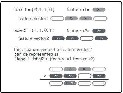
In algorithm 1, theΦfunction generates a feature vec-tor from a label and an instance. ⊕denotes an opera-tor that concatenates two vecopera-tors,mdenotes the label length, andyidenotes a label element. We define the Φfunction as follows,
Φ(y,x) = (y1x)⊕(y2x)⊕ · · · ⊕(ymx).
For example, for a given pair
y = (1,0,1,0),x = (1,2,3,4) , we obtain
each label element. That is, the weights of each fea-ture can be determined for each label element. We can decide whether the feature is a positive evidence or a negative evidence for each label element.
• cost function
We define three cost functions for the labels, each one of which is represented as a binary vector. Section 6 explains the cost functions in detail.
5 Transformation of the polynomial
kernel
As a kernelized learner, we often use a polynomial kernel in NLP in order to treat the combination of features such as words and dependencies. Letmbe the label length, and
K(v,v0)be apdegree polynomial kernel. We transform
this kernel to reduce the computational complexity. The transformation is composed of integrating theΦfunction and polynomial kernel, and decomposing the integrated kernel.
5.1 Integrating the
Φ
function and the kernel
Let us first consider reducing the computational complex-ity per kernel function evaluation. For calculating the ker-nel, we must regenerate the feature vector from xandy, or cache the kernel values. However it is impractical to hold all theN2mfeature vectors. In addition, we must deal
with all feature vectors at each iteration. The access to fea-ture vectors does not have locality of reference. Therefore caching support vectors is not efficient. For this reason, we calculate the kernel value directly, by integrating the poly-nomial kernel and theΦfunction.
Let us calculate the kernel between the vectors generated by theΦfunction in due order. For simplicity, the constant term in the polynomial kernel is dropped out, without loss of generality. Thepdegree polynomial kernel can be ex-panded as follows:
K(Φ(y,x),Φ(y0,x0))
= ((y1·x⊕y2·x⊕. . .⊕ym·x)· (y0
1·x0⊕y02·x0⊕. . .⊕y0m·x0))p.
Since in the kernel space an inner product can be obtained by the range of features corresponding to each label ele-ment, the above formula can be tranformed as follows:
K(Φ(y,x),Φ(y0,x0)) =
{(y1·y01)(x·x0) +. . .+ (ym·y0m)(x·x0)}p,
and we can extract the products of the dot-product of in-stance vectors(x·x0),K(Φ(y,x),Φ(y0,x0)) = ((y·y0)(x· x0))p.Thus, a kernel can be represented by a dot-product
of labels (y·y0) and a dot-product of instance vectors
(x·x0). It turns out that we can evaluate the polynomial
ker-nel without theΦfunction. Here, let the kernel integrated withΦfunction be denoted byKexas follows:
Kex(y,x,y0,x0) = ((y·y0)(x·x0))p. (2)
Refer to Figure 1 for intuitive explanation. Through the kernel integrated withΦ, we can evaluate a kernel by only the dot-product between the instance vectors, regardless of the label length.
If we do not integrateΦwith the kernel, evaluation of the kernel costs(label length)×(feature size) computa-tional time and memory. By contrast, evaluation costs only
Fig. 1:IntegratingΦfunction and kernel
(label length) + (feature size)for both in our calculation. Since we have to only cache the kernel between the in-stances, cache efficiency increases significantly.
5.2 Decomposing the kernel
In order to reduce the number of calls to the kernel function as much as possible, we expand the integrated kernel fur-ther, limiting ourselves to the case of second degree poly-nomial kernels for the sake of simplicity.
In the Passive Aggressive Algorithm with a kernel, the number of suppor vectors increases during the iterations, and becomes an arbitrarily large set. For this problem, Moh (2008) proposed a method that expands a second degree polynomial kernel to an induced feature space, and treated it as a linear model to avoid treating support vectors for memory complexity. However, since Moh’s method must treat a large space that is of a square of the size of a fea-ture set, this has the opposite effect that the computational space is increasing. Thus, this method cannot treat a large number of features. If we expand the kernel in a feature space, it cannot benefit from the kernel trick and it must treat a large feature space as in Moh(2008). We expand the kernel not only in the feature space, but also in the label space. Therefore, we can expand the kernel efficiently, if
label length<feature size.
Kexcan be decomposed and represented as a
combina-tion ofyithat belongs toy, where the constant term in a
polynomial kernel is dropped out without loss of general-ity,
Kex(y,x,y0,x0)=((y·y0)(x·x0))2=(y)2((y0)2(x·x0)2).
Here, we consider the calculation of the kernel score
S(y,x)between an example(y,x)and the support vec-tors{τ(t),y(t),x(t)}. We decomposeyandy(t) to each yi and y(it), and expand the square. So let γij denote ∑
{t|(τ(t),y(t),x(t))∈W}τ(t)yi(t)y(jt)(x·x(t))2, becauseγij
is constant in terms ofy. We then obtain the score of the example:
S(y,x) = ∑
(τ(t),y(t),x(t))∈W
τ(t)Kex(y,x,y(t),x(t))
= ∑
{i,j|i6=j, i,j<m}
yiyjγij+ ∑
{i|i≤m} y2
iγii.
As shown above, support vectors can box in the parame-ters γ ∈ Rm2
same model, we can calculate the score usingγfor eachy
without calls to the kernel. We call the expanded kernel a “transformed kernel”.
5.3 Predicting with polynomial kernelization
At step 4 of Algorithm 1, we solve the maximization prob-lem. We exploit the expansion so that we obtain the label which violates the constraints to the highest extent.
Algorithm 2 predictsy¯using the transformed kernel. 1
denotes the label, each element of which is 1. eidenotes
a label that is the vector with a1in thei-th element and 0 elsewhere. And τ(k) denotes the weight on thek-th
sup-port vector.svki= Φ(ei,SVk)denotes the feature vector
generated by Φfrom thek-th support vector andei. We
henceforth definey(0)as always equal to 1, so that we
cal-culateγwith a constant term, and the label whose length is
mimplicitly includes the constant termy(0).
Algorithm 2for findingy¯.
Input: x= Φ(1,x), τ,W={SV1,...,SVn}
Input: true y//correct label(in training only) 1: for all {(i, j)|0< i≤j≤m} do 2: γij=
∑
svk∈W
τ(t)β
ijK(svki,x)K(svkj,x)
βij= {
1 if(i=j) 2 otherwise
3: end for
4: for 0≤i≤mdo 5: γ0i=γi0=
∑
svk∈W
τ(t)K(sv
ki,x)
// processing constant terms. 6: end for
7: y¯= argmax
y∈{0,1}mS(y,x) //when classifying
¯
y= argmax
y∈{0,1}mS(y,x) +ρ(true y,y) //when training 8: return(¯y)
Calculatingγrequires calling the kernel functionn(m+ 1)2times, but the evaluation of each label requires only the
calculation of the polynomial expression whose coefficient is γ. Thus, even the evaluation of all possible labels has only to call the kerneln(m+ 1)2times.
Additionally, the Passive Aggressive Algorithm trains the model incrementally, and the weight of the support vec-tor added to the model does not change. In this way, if we holdγfor all instances,γcan be updated according to the support vectors newly added to the model. Thus, complex-ity can be reduced even further.
5.4 Discussion
Here, we discuss the computational complexity of the learning. LetNbe the number of examples, and lethbe the number of support vectors included in the model at a given point. LetH be the number of the final support vectors,
I be the number of iterations needed to obtainHsupport vectors, andmbe the label length.
We assume that the misclassification rate of training data is constant while training the model. We then need to per-form classification calculationλ = N I
H times in order to
obtain one support vector. In the following, we will see the number of calls to the kernel required to obtain all the
support vectors for each case of without transformation and with transformation.
• Without kernel transformation
Since evaluation of each example requiresh2mcalls
to the kernel function, obtaining one support vector requiresh2mλcalls. Thus, the number of calls to the
kernel to obtainHsupport vectors is,∑Hh=1hλ2m=
NI(H+ 1)2m−1.In practice, misclassifications
de-crease in number with training and one support vector requires more classification examples. Hence com-plexity can become larger.
• When transforming the kernel
Since evaluation of the examples requires only the cal-culation of the kernel of the new support vectors, it needs H(mI+1)2 calls to the kernel function on aver-age. Therefore, the number of calls to the kernel to get
Hsupport vectors is,HH(mI+1)2λ=NH(m+ 1)2.
In the cases where the label length is long or training needs many iterations, the computational complexity ben-efits from the transformation of the kernel.
6 Cost function
In structured output learning, for a given pair of labels, a cost is calculated by a cost function. Hereby, we can in-troduce a “near error” and a “distant error”, and impose a little penalty to near error and a large penalty to distant error. We define three cost functions. Each cost function defines what is ”near” and ”distant”.sis a scale parameter in the following.
• 0/1 cost
ρ0/1(y,y0) = {
0 ify=y0 s otherwise
It returnssif the labels differ, and 0 otherwise. It is the most basic cost function that can be defined for general labels.
• average cost
ρaverage(y,y0) = m1 ∑mi=1 {
0 if y(i)=y0(i) s otherwise
It returnss×(the number of different elements in the label)divided by the label length. It means that errors in several label elements induce a larger penalty.
• Asymmetric cost
ρasm(y,y0) = m1 m ∑
i=1
0 y(i)=y0(i) s·ji y(i)= 1, y(i)6=y0(i)
s otherwise
This cost function returnss·jiif a positive element
Table 1:Dialogue example
A wait, is this a computer science conference ? A or is it a
B um, well, it’s more . . . B it’s both right.
B it’s it’s sort of t- cognitive neural psycho linguistic B but all for the sake of doing computer science B so it’s sort of cognitive psycho neural plausibly
motivated architectures of natural language processing B so it seems pretty interdisciplinary
reserved. We assign different parametersji to each
label, so that this function can absorb the positive and negative bias that is different for each element.
7 Experiments
We examine the task of identifying agreement and dis-agreement between utterances to verify the efficiency and the effectiveness of our method. Identifying agreement and disagreement between utterances is to predict whether each utterance shows agreement or disagreement, and inter-utterances have a link.
7.1 Data
We used the MRDA corpus that has been used by related works (Galley, 2004). This corpus contains dictated text and audio data collected from 75 multi-party meetings in ICSI. The meetings, one hour duration each, have been held on a weekly basis by 6.5 researchers on average. For all utterances in this corpus, annotators labeled that the Dialog Acts, speakers, Adjacency-Pairs, etc.
Each Dialog Act is a category of utterances defined ac-cording to their intent. There are 44 Dialog Acts. Among them, we regard 4 tags, Acknowledge-answer(“bk”), Ac-cept(“aa”), Accept-part(“aap”), Maybe(“am”), as agree-ment. We regard other 2 tags, Reject(“ar”), Reject-part(“arp”) as disagreement. Adjacency-Pairs are another kind of tags. We regard an utterance pair is linked if they are annotated with the Adjacency-Pairs tag. We show the dialogue example in Table 1.
7.2 Experimental settings
In this experiment, we aim to predict the agreement and disagreement relations between the utterances, segmented into groups of 3 continuous utterances: first, second, and third utterances. There are 3 possible links. For each link, there are 3 possible values: agreement, disagreement, oth-ers. Therefore, the label lengthmis9. In this paper, we train and classify shifting the segments by 1 utterance. That is, the second utterance from an example is the first utter-ance on the next example. We also used as features the preceeding and succeeding 3 utterances, 7 utterance in all, to classify on our method. The features that denote the content of utterances are the word length, uni-grams, bi-grams, tri-bi-grams, head 2 words, and tail 2 words. The fea-tures that denote relations between utterances are whether the speaker is the same or not, and the time interval. We cannot evaluate this problem precisely by accuracy, since the classes are biased in size. Thus, we used F-value in order to evaluate. We used 12499 examples to train, and 9200 examples for testing. We do not determine an itera-tion limit in the Passive Aggressive Algorithm; instead, we
used the model of the point of convergence. The second degree polynomial kernel was used, and the constant term is set to 1.
7.3 Execution time
We also measure the execution time. When the kernel is not integrated, the execution time tends to be prohibitively long. So we experimented with a small training dataset in that case.
Additionally, we used fixed parameters, because param-eters influence the execution time. The number of iterations is 15. We used the average cost. We set the scale factor of the cost functionsto 10. We used the second degree poly-nomial kernel in the evaluations of both the transformed and non-transformed kernels.
8 Results
8.1 Effect of the cost function
We show the result of our examination of the performance of the cost function in Table 2. We first compare the re-sult with the zero-one cost with the rere-sult with the average cost. When the zero-one cost is used, the utterance posi-tion changes the result significantly, but classifying each position utterance is the same problem.
On the other hand, when the average cost is used, the utterance position does not change results much. Since the zero-one cost judges only the overall correctness of the predicted relations, it learns to reserve margin against both near errors and distant errors. As a result, it reserves over-sized margin against mistakes of the label elements during learning. But, when the average cost is used, the mistakes of label elements change the score; So it learns to reserve an appropriate margin against elements of each label.
Furthermore, when the asymmetric cost is used, the method performs well for all label elements. This is be-cause this asymmetric cost absorbs the proportion of pos-itive contents and negative contents, by implementing dif-ferential penalty for the mistakes. We show the effect of the parameters of asymmetric cost in the next section.
Table 2:Performance of the cost function
Cost function 0/1 Average Asymmetric(j=3) Agreement (utterance 1) 0.337 0.394 0.490 Agreement (utterance 2) 0.170 0.343 0.462 Agreement (utterance 3) 0.097 0.237 0.414 Disagreement (utterance 1) 0.016 0.000 0.134 Disagreement (utterance 2) 0.000 0.032 0.032 Disagreement (utterance 3) 0.000 0.000 0.076 Link( utterance 1-2 ) 0.030 0.074 0.305 Link( utterance 2-3 ) 0.021 0.088 0.366 Link( utterance 1-3 ) 0.012 0.083 0.277
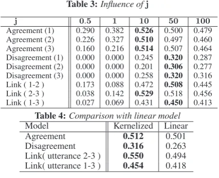
8.2 Effect of the parameters
j
We show the results with different values of parameters
j ∈ {ji}min Table 3. We can change the penalty that is
Table 3:Influence ofj
j 0.5 1 10 50 100
Agreement (1) 0.290 0.382 0.526 0.500 0.479 Agreement (2) 0.226 0.327 0.510 0.497 0.460 Agreement (3) 0.160 0.216 0.514 0.507 0.464 Disagreement (1) 0.000 0.000 0.245 0.320 0.287 Disagreement (2) 0.000 0.000 0.201 0.306 0.277 Disagreement (3) 0.000 0.000 0.258 0.320 0.316 Link ( 1-2 ) 0.173 0.088 0.472 0.508 0.445 Link ( 2-3 ) 0.038 0.142 0.529 0.518 0.456 Link ( 1-3 ) 0.027 0.069 0.431 0.450 0.413
Table 4:Comparison with linear model
Model Kernelized Linear
Agreement 0.512 0.501
Disagreement 0.316 0.263
Link( utterance 2-3 ) 0.550 0.494
Link( utterance 1-3 ) 0.454 0.418
8.3 Effect of the kernel
Based on the results above, we optimized the weightjfor agreement/disagreement and link, and compared with the linear model. The weight parameters are as follows:
jyea = 3,jnay = 10,jlink1−2,2−3 = 6, jlink1−3 = 5.
We set the scale factor of the cost function s to 5. In linear model: jyea = 3,jnay = 100,jlink1−2,2−3 = 6,
jlink1−3 = 5. We set the scale factor of linear model
slinearto 4. We chose the parameters for test data. Thus,
the results are the upper limit that we can obtain by tuning the parameters.
We show the results with this settings in Table 4. The lin-ear model cannot deal with corresponding words among the utterances because it cannot treat a combination of features, and slows down the performance, especially when classi-fying links. In classification of agreements/disagreements, the polynomial kernel improves the performance, too.
8.4 Computational complexity
We measured the execution times and compared them in Table 5. For both cases of using transformation or not, the execution time is proportional to (example size)×
(support vector size).
Without overheads, the difference of these execution times is close to the theoretical complexity difference when the kernel is called2m= 512times and the complexity for
each kernel ism = 9times higher, coming together as in total 4608 times.
Table 5:Execution time
Number of training examples 50 100 150
Support vectors 118 183 294
Using non-transformed kernel 15523s 56227s 139590s Using transformed kernel 3. 19s 8.14s 28.65s
Ratio ×4866 ×6907 ×4872
9 Conclusion
In this paper, we proposed the cost functions to take into account the different class proportions between the prob-lems, and a method that transforms the kernel to reduce the computational complexity of learning with structured out-put and kernels. This algorithm is based on one of the on-line max margin algorithm, Passive Aggressive Algorithm, so it learns fast and uses a small amount of memory. We evaluated our method on the task of identifying agreement and disagreement relations, and we empirically and theo-retically showed the computational complexity of the
pro-posed method, and also the efficiency of using a polyno-mial kernel for structured output learning.
References
[1] Koby Crammer, Ofer Dekel, Joseph Keshet, Shai Shalev-Shwartz, Yoram Singer, Online Passive-Aggressive Algo-rithms.Journal of Machine Learning Research, Vol. 7, pp. 551–585, 2006.
[2] Michel Galley, Kathleen McKeown, Julia Hirschberg, Eliz-abeth Shriberg, Identifying agreement and disagreement in conversational speech: Use of bayesian networks to model pragmatic dependencies. InProceedings of the 42nd Annual Meeting on Association for Computational Linguistics, pp. 669–676, 2004.
[3] Taku Kudo, Yuji Matsumoto, Japanese dependency struc-ture analysis based on support vector machines. In Proceed-ings of the 2000 Joint SIGDAT Conference on Empirical Methods in Natural Language Processing and Very Large Corpora, pp. 18–25, 2000.
[4] Elizabeth Shriberg, Raj Dhillon, Sonali Bhagat, Jeremy Ang, and Hannah Carvey, The ICSI meeting recorder di-alog act (MRDA) corpus. InProceedings of the 5th SIGdial Workshop on Discourse and Dialogue, pp. 97–100, 2004. [5] Ioannis Tsochantaridis, Thomas Hofmann, Thorsten
Joachims, Yasemin Altun, Support Vector Learning for In-terdependent and Structured Output Spaces. InProceedings of the 21st International Conference on Machine Learning, pp. 823–830, 2004.
[6] Yasemin Altun, Ioannis Tsochantaridis, Thomas Hofmann, Hidden Markov Support Vector Machines. InProceedings of the 20th International Conference on Machine Learning, pp. 3–10, 2003.
[7] Yvonne Moh,Thorsten, Joachim Buhmann, Kernel Expan-sion for Online Preference Tracking. Inproceedings of The International Society for Music Information Retrieval, pp. 167–172, 2008.
[8] Ioannis Tsochantaridis, Thomas Hofmann, Thorsten Joachims, Yasemin Altun, Support Vector Learning for in-dependent and Structured Output Spaces. InProceedings of the 21st International Conference on Machine Learning, p. 104 , 2004.
[9] Francesco Orabonal, Joseph Keshet, Barbara Caputo, The projectron: a bounded kernel-based Perceptron. In Pro-ceedings of the 25th International Conference on Machine Learning, pp. 720–727 , 2008.
[10] Jiampojamarn Sittichai, Cherry Colin, Kondrak Grzegorz, Joint Processing and Discriminative Training for Letter-to-Phoneme Conversion. In Proceedings of 2008 Annual Meeting on Association for Compurational Linguistics and Human Language Technology Conference, pp. 905–913, 2008.
[11] S. Sathiya Keerthi, Olivier Chapelle, Dennis DeCoste, Building Support Vector Machines with Reduced Classifier Complexity.The Journal of Machine Learning Research, Volume 7, pp. 1493–1515, 2006.