Comparative Study between Various Classification Algorithms for Classification of Cardiotocogram Data

(1)

CSEIT1724172 | Received : 10 August 2017 | Accepted : 21 August 2017 | July-August-2017 [(2)4: 651-657]

651

Comparative Study between Various Classification Algorithms

for Classification of Cardiotocogram Data

Jagannathan D

M.Phil. (PG Scholar), Department of Computer Science, Dr. C. V. Raman University, Chhattisgarh, India

ABSTRACT

Cardiotocography (CTG) is a simultaneous recording of fetal heart rate (FHR) and uterine contractions (UC). It is one of the most common diagnostic techniques to evaluate maternal and fetal well-being during pregnancy and before delivery. By observing the Cardiotocography trace patterns doctors can understand the state of the fetus. There are several signal processing and computer programming based techniques for interpreting a typical Cardiotocography data. Even few decades after the introduction of cardiotocography into clinical practice, the predictive capacity of the these methods remains controversial and still inaccurate. In this paper, we implement a model based CTG data classification system using a supervised SVM, Decision Tree, MLP and Navie Bayes which can classify the CTG data based on its training data. We used specificity, NPV, Precision, Recall, G-Mean, F-Measure and ROC as the metric to evaluate the performance. It was found that, the ANN based classifier was capable of identifying Normal, Suspicious and Pathologic condition, from the nature of CTG data with very good accuracy.

Keywords : CTG, Data mining, Classification, Support Vector Machine, Decision Tree, Multilayer Perceptron and Navie Bayes.

I. INTRODUCTION

Data mining and knowledge discovery in databases (KDD) are extracting novel, understandable and useful information, knowledge or patterns from huge amount of available data. In the other words, data mining has capabilities for analyzing the large datasets, finding unexpected or hidden relationships between various attributes and summarizing the extracted information more understandable and useful to data users or owners. In the traditional model for transforming data to knowledge, some manual analysis and interpretation are executed. For example, in medical centers, generally doctors or specialists manually analyze current trends, disease and health-care data, then make a report and use this report for decision making or planning for medical diagnosis, treatments and etc. The problem of this type of data analysis is that, this form of manual data analysis is slow, expensive, time consuming, and highly subjective.

Data mining has two main tasks:

Predictive tasks: with applying various techniques or algorithms, it can make decisions or predict the unknown or future values of other variables. This technique includes classification, association rule and etc.

Descriptive tasks: describe the data or find human understandable patterns and present the results in tables, diagrams and etc., which can be understand easily by data owners or data users.

(2)

data mining is to haul new and previously unknown clinical solutions and patterns to aid the clinicians in diagnosis, prognosis and therapy. Moreover application of software solutions to store patient records in an electronic form is expected to make mining knowledge from clinical data less stressful .

Figure 1. Examples of CTG trace FHR(top) and utrine activity(bottom)

Cardiotocography (CTG), consisting of Fetal Heart Rate (FHR) and Tocographic (TOCO) measurements, is used to evaluate fetal well-being during the delivery.FHR patterns are observed manually by obstetricians during the process of CTG analyses. For the last three decades, great interest has been paid to the fetal heart rate baseline and its frequency analysis. Fetal Heart Rate (FHR) monitoring remains widely used as a method for detecting changes in fetal oxygenation that can occur during labor. Yet, deaths and long-term disablement from intrapartum hypoxia remain an important cause of suffering for parents and families, even in industrialized countries. Confidential inquiries have highlighted that as much as 50% of these deaths could have been avoided because they were caused by non-recognition of abnormal FHR patterns, poor communication between staff, or delay in taking appropriate action. Computation and other data mining techniques can be used to analyze and classify the CTG data to avoid human mistakes and to assist doctors to take a decision.

II. DATASET DESCRIPTION

The cardiotocography data set used in this study is publicly available at ―The Data Mining Repository of University of California Irvine (UCI)‖. By using 21 given attributes data can be classified according to FHR pattern class or fetal state class code. In this study, fetal state class code is used as target attribute instead of FHR pattern class code and each sample is classified

into one of three groups normal, suspicious or pathologic. The dataset includes a total of 2126 samples of which is 1655 normal, 295 suspicious and 176 pathologic samples which indicate the existing of fetal distress.

Attribute information is given as:

LB—FHR baseline (beats per minute) AC—# of accelerations per second FM—# of fetal movements per second UC—# of uterine contractions per second DL—# of light decelerations per second DS—# of severe decelerations per second DP—# of prolongued decelerations per second

ASTV—percentage of time with abnormal short term variability

MSTV—mean value of short term variability ALTV—percentage of time with abnormal long term

variability

MLTV—mean value of long term variability Width—width of FHR histogram

Min—minimum of FHR histogram Max—Maximum of FHR histogram Nmax—# of histogram peaks Nzeros—# of histogram zeros Mode—histogram mode Mean—histogram mean Median—histogram median Variance—histogram variance Tendency—histogram tendency

CLASS—FHR pattern class code (1 to 10)

NSP—fetal state class code (N = normal; S = suspect; P = pathologic)

III. CLASSIFICATION

Classification is called as supervise learning. It take some of data (named as training set) which has collection of records and each record contain set of attributes and define one attribute named as class. The main goal of classification is producing a model with capability of predicting the value of class attribute in previously unseen records as accurately as possible. A test set is used for predicting the accuracy of the created model. Some applications of classification in medical diagnosis are: classifying tumor cells, analyzing the effectiveness of treatment and etc.

(3)

C4.5, Hunt’s Algorithm and etc.,), Rule-Based Methods, Memory-Based Methods (such as: k-Nearest-Neighbor), Genetic Programming, Naïve Bayes and Bayesian Classification, Artificial Neural Networks, Support Vector Machines (SVMs), Ensemble Methods and etc.

3.1 Support Vector Machine

Support Vector Machine (SVM) is a supervised machine learning algorithm which can be used for both classification and regression challenges. However, it is mostly used in classification problems. In this algorithm, we plot each data item as a point in n-dimensional space (where n is number of features you have) with the value of each feature being the value of a particular coordinate. Then, we perform classification by finding the hyper-plane that differentiates the two classes very well. The black line that separate the two cloud of class is right down the middle of a channel.The separation is In 2d, a line, in 3D, a plane, in four or more dimensions an a hyperplane. Mathematically, the separation can be found by taking the two critical members, one for each class. This points are called support vectors. These are the critical points (members) that define the channel.The separation is then the perpendicular bisector of the line joining these two support vectors. That's the idea of support vector machine.

Figure 2. Optimal hyper plane separating the two classes

SVM Algorithm

Algorithm: Generate SVM

Input: Training Data, Testing Data Output: Decision Value

Method:

Step 1: Load Dataset

Step 2: Classify Features (Attributes) based on class labels

Step 3: Estimate Candidate Support Value While (instances! =null)

Do

Step 4: Support Value=Similarity between each instance in the attribute

Find Total Error Value Step 5: If any instance < 0 Estimate

Decision value = Support Value\Total Error Repeat for all points until it will empty End If

3.2 Navie Bayes

The Naive Bayes Classifier technique is based on the so-called Bayesian theorem and is particularly suited when the dimensionality of the inputs is high. Despite its simplicity, Naive Bayes can often outperform more sophisticated classification methods.

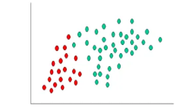
To demonstrate the concept of Naïve Bayes Classification, consider the example displayed in the illustration above. As indicated, the objects can be classified as either GREEN or RED. Our task is to classify new cases as they arrive, i.e., decide to which class label they belong, based on the currently exiting objects.

Since there are twice as many GREEN objects as RED, it is reasonable to believe that a new case (which hasn't been observed yet) is twice as likely to have membership GREEN rather than RED. In the Bayesian analysis, this belief is known as the prior probability. Prior probabilities are based on previous experience, in this case the percentage of GREEN and RED objects, and often used to predict outcomes before they actually happen.

Optimal Hyperplane X

2

Maxim um margin X

(4)

Thus, we can write:

Since there is a total of 60 objects, 40 of which are GREEN and 20 RED, our prior probabilities for class membership are:

Having formulated our prior probability, we are now ready to classify a new object (WHITE circle). Since the objects are well clustered, it is reasonable to assume that the more GREEN (or RED) objects in the vicinity of X, the more likely that the new cases belong to that particular color. To measure this likelihood, we draw a circle around X which encompasses a number (to be chosen a priori) of points irrespective of their class labels. Then we calculate the number of points in the circle belonging to each class label. From this we calculate the likelihood:

From the illustration above, it is clear that Likelihood of X given GREEN is smaller than Likelihood of X given RED, since the circle encompasses 1 GREEN object and 3 RED ones. Thus:

Although the prior probabilities indicate that X may belong to GREEN (given that there are twice as many GREEN compared to RED) the likelihood indicates otherwise; that the class membership of X is RED (given that there are more RED objects in the vicinity of X than GREEN). In the Bayesian analysis, the final

classification is produced by combining both sources of information, i.e., the prior and the likelihood, to form a posterior probability using the so-called Bayes' rule (named after Rev. Thomas Bayes 1702-1761).

Finally, we classify X as RED since its class membership achieves the largest posterior probability. Naive Bayes can be modeled in several different ways including normal, lognormal, gamma and Poisson density functions:

The Naive Bayesian classifier is based on Bayes’ theorem with independence assumptions between predictors. A Naive Bayesian model is easy to build, with no complicated iterative parameter estimation which makes it particularly useful for very large datasets. Despite its simplicity, the Naive Bayesian classifier often does surprisingly well and is widely used because it often outperforms more sophisticated classification methods.

3.3 Decision Tree

(5)

branches (e.g., Sunny, Overcast and Rainy). Leaf node (e.g., Play) represents a classification or decision. The topmost decision node in a tree which corresponds to the best predictor called root node. Decision trees can handle both categorical and numerical data.

A decision tree is built top-down from a root node and involves partitioning the data into subsets that contain instances with similar values (homogenous). ID3 algorithm uses entropy to calculate the homogeneity of a sample. If the sample is completely homogeneous the entropy is zero and if the sample is an equally divided it has entropy of one.

To build a decision tree, we need to calculate two types of entropy using frequency tables as follows:

a) Entropy using the frequency table of one attribute:

b) Entropy using the frequency table of two attributes:

The information gain is based on the decrease in entropy after a dataset is split on an attribute. Constructing a decision tree is all about finding attribute that returns the highest information gain (i.e., the most homogeneous branches).

Step 1: Calculate entropy of the target.

Step 2: The dataset is then split on the different attributes. The entropy for each branch is calculated. Then it is added proportionally, to get total entropy for the split. The resulting entropy is subtracted from the entropy before the split. The result is the Information Gain, or decrease in entropy.



T X



Entropy

 

T Entropy



T X



Gain ,   ,

Step 3: Choose attribute with the largest information gain as the decision node.

Step 4a: A branch with entropy of 0 is a leaf node. Step 4b: A branch with entropy more than 0 needs further splitting.

Step 5: The ID3 algorithm is run recursively on the non-leaf branches, until all data is classified.

3.4 Multilayer Perceptron

Multilayer perceptron classifier (MLPC) is a classifier based on the feed forward artificial neural network. MLPC consists of multiple layers of nodes. Each layer is fully connected to the next layer in the network. Nodes in the input layer represent the input data. All other nodes maps inputs to the outputs by performing linear combination of the inputs with the node’s weights ww and bias bb and applying activation function. A multi-layer perceptron (MLP) has the same structure of a single layer perceptron with one or more hidden layers. The backpropagation algorithm consists of two phases: the forward phase where the activations are propagated from the input to the output layer, and the backward phase, where the error between the observed actual and the requested nominal value in the output layer is propagated backwards in order to modify the weights and bias values.

It can be written in matrix form for MLPC with K+1K+1 layers as follows:

y(x)=fK(...f2(wT2f1(wT1x+b1)+b2)...+bK)y(x)=fK(...f 2(w2Tf1(w1Tx+b1)+b2)...+bK)

Nodes in intermediate layers use sigmoid (logistic) function:

f(zi)=11+e−zif(zi)=11+e−zi

Nodes in the output layer use softmax function: f(zi)=ezi∑Nk=1ezkf(zi)=ezi∑k=1Nezk

The number of nodes NN in the output layer corresponds to the number of classes.

IV. EXPERIMENTATION RESULT

4.1 Performance Evaluation

This is a measurement tool to calculate the performance

Accuracy = _ _

  



FN FP TN TP

TN TP

Sensitivity = _ _ FN TP

(6)

Specificity =_ _ proportion of positive cases that were correctly identified

 The false positive rate (FP) is the proportion of negatives cases that were incorrectly classified as positive

number of predictions that were correct.

 The Sensitivity or Recall the proportion of

actual positive cases which are correctly identified.

 The Specificity the proportion of actual

negative cases which are correctly identified.

 The Positive Predictive Value or Precision the

proportion of positive cases that were correctly identified.

 The Negative Predictive Value the proportion

of negative cases that were correctly identified.

Decision Tree

SVM Navie Bayes

MLP

Accuracy 97.4130 97.9304 84.8542 98.256 Sensitivity 95.4520 96.9135 70.9042 97.544 Specificity 97.7919 99.2001 85.5353 99.231 PPV 95.8897 95.5561 72.5203 97.356 NPV 97.6064 97.7207 98.235 98.354 ROC 89.9895 98.0568 78.2197 98.155

V. CONCLUSION

This work has evaluated the performance of the four methods with respect to confusion matrix and accuracy. The performance neural network based classification model has been compared with SVM, DT, NB and MLP. According to the arrived results, the performance of the supervised machine learning based classification approach provided significant performance. It was found that the DT classifier was capable of identifying Normal, Suspicious and Pathologic condition, from the nature of CTG data with very good accuracy. This work trains the system with all the classes of samples, there is a chance by which the trained system may be incapable of identifying suspicious record. That is why we are getting comparatively poor average performance while classifying suspicious records. It is a major weakness of the system and it should be overcomes in future design. One may address the way to improve the system for getting proper training with different classes of CTG patterns. Future works may address hybrid models using statistical and machine learning techniques for improved classification accuracy.

VI. REFERENCES

[1]. G. Georgoulas, D. Stylios, P. Groumpos, Predicting the risk of metabolic acidosis for new borns based on fetal heart rate signal classiﬁcation using support vector machines, IEEE Trans. Biomed. Eng. 53 (2006) 875–884. [2]. S.L. Salzberg, On comparing classiﬁers: pitfalls

to avoid and a recommended approach, Data Min. Knowl. Discov. (2007) 317–328.

[3]. M. Cesarelli, M. Romano, P. Bifulco, Comparison of short term variability indexes in cardiotocographic fetal monitoring, Comput. Biol. Med. 39 (2009) 106–118.

[4]. K. Bache, M. Lichman, Cardiotocography data set, in: UCI Machine Learning Repository, 2010. http://archive.ics.uci.edu/ml/datasets/cardiotocog raphy

[5]. N. Krupa, M. Ali, E. Zahedi, S. Ahmed, F.M. Hassan, Antepartum fetal heart rate feature extraction and classiﬁcation using empirical mode decomposition and support vector machine, Biomed. Eng. Online 10 (2011) 6. [6]. R. Czabanski, J. Jezewski, A. Matonia, M.

(7)

rate signals as the predictor of neonatal acidemia, Expert Syst. Appl.39 (2012) 11846–11860. [7]. C. Sundar . "Performance Evaluation of K-Means

and Hierarchal Clustering in Terms of Accuracy and Running Time. "International Journal Computer Science Application (2012)

[8]. E. Yilmaz, C. Kilikcier, Determination of fetal state from cardiotocogram using LS-SVM with particle swarm optimization and binary decision tree, Comput. Math. Methods Med. 2013 (2013) 487179.

[9]. Tomas Peterek, Petr Gajdos, Pavel Dohnalek, Jana Krohova, Human Fetus Health Classification on Cardiotocographic Data Using Random Forests , Intelligent data analysis and its applications , volume II,pp:189-198,(2014) [10]. Hakan Sahin∗, Abdulhamit Subasi ,

Classiﬁcation of the cardiotocogram data for anticipation of fetal risks using machine learning techniques , International Burch University, Faculty of Engineering and Information Technologies, Francuske Revolucije b.b., Ilidza, Sarajevo 71000, Bosnia and Herzegovina, Applied Soft Computing 33 (2015) 231–238. [11]. V.N. Vapnik and A. Chervonenkis, "A note on

one class of perceptrons", Automation and Remote Control, 25, 1964

[12]. J.R.Quinlan, "Induction of decision tree". Journal of Machine Learning 1, 1986, Pg.no:81-106. [13]. V. N. Vapnik, "The Nature of Statistical

Learning Theory", Springer, New York, NY, USA, 1995.

[14]. Mark A. Hall, Lloyd A. Smith, Feature Subset Selection: A Correlation Based Filter Approach, In 1997 International Conference on Neural Information Processing and Intelligent Information Systems (1997), pp. 855-858.

[15]. Han and Kamber, - "Data Mining; Concepts and Techniques", Morgan Kaufmann Publishers, 2000.