Robust Dynamic Mechanisms

(1)

Robust Dynamic Mechanisms

Thesis by

Mohamed Mostagir

In Partial Fulfillment of the Requirements for the Degree of

Doctor of Philosophy

California Institute of Technology Pasadena, California

2012

(2)

(3)

Acknowledgements

The following people and places have made my time at Caltech an educational and enjoyable expe-rience.

Mentors: John Ledyard, Preston McAfee, Tom Palfrey, and Jean-Laurent Rosenthal. Further advice from Marina Agranov, Colin Camerer, Federico Echenique, Erik Snowberg, Leeat Yariv, and Adam Wierman.

Friends: Greg and Pia, Dustin and Katya, Sera, Ines, Salvo, Julian, Gui, Andrea, Maggie, Boosey, Marjan, Andrej, Ian, Marwa Mabrouk, Dani and Gabri, Lisa and Costia, Xiao Jun.

Friends-at-a-distance: Theo, Katy, Peach, Khaldoun, and Kostas.

Student Life: Tim! Sue, Barbara, John, Geoff, Mike, Juan, and all the wonderful people at Caltech Housing.

Administrative: Edith, Laurel, Suzanne, Gloria, Gail, Sheryl, and Victoria. The Mediterranean Cafe!

Lloyd House: the highlight of my time at Caltech. I live and die for those I love. Family: Mesbah, Mona, and Mai.

I have spent the best years of my life in Pasadena. This in no small part was due to the fact that my days were consistently brightened up by Hadil’s exuberant presence. Laila Hikaru made her appearance towards the end and life became even more beautiful. I would dedicate this thesis to the two of them, but I will instead save that for my best work, which is still ahead of me.

(4)

Abstract

This thesis presents and solves two dynamic problems. The first problem comes from online display advertising. In display advertising, a publisher displays an ad for an advertiser when a targeted user visits a webpage related to the advertiser’s products or services. However, the publisher cannot control the supply of display opportunities, and hence the actual supply of ads that it can sell is stochastic. I consider the problem of optimal ad delivery, where the advertiser demands a certain number of impressions to be displayed over a certain time horizon. Time is divided into periods, and in the beginning of each period the publisher chooses a fraction of the still unrealized supply to allocate towards fulfilling the publisher’s demand. The goal is to be able to fulfill the demand at the end of the horizon with minimal costs incurred from penalties associated with shortage or overdelivery of impressions. For a special case of this problem I describe an optimal policy that is very easy to implement. The general version of the problem is more computationally demanding, but I describe policies that are both implementable and arbitrarily close to the optimal solution.

(5)

(6)

Contents

Acknowledgements iii

Abstract iv

1 Introduction 1

1.1 Display Advertising . . . 2

1.1.1 Contribution . . . 3

1.1.2 Methodology . . . 4

1.2 Exploiting Myopic Learning . . . 5

1.3 Best Response and Fictitious Play . . . 6

2 Optimal Delivery in Display Advertising 9 2.1 Introduction . . . 9

2.2 Model and Notation . . . 12

2.3 Single Advertiser . . . 15

2.4 Single Advertiser — General Case . . . 21

2.5 Extensions . . . 28

(7)

2.5.2 Additional Delivery Constraints . . . 31

2.6 Discussion . . . 32

3 Exploiting Myopic Learning 34 3.1 Introduction . . . 34

3.2 Model . . . 38

3.2.1 The Cheat-Audit Game . . . 39

3.2.2 Learning Dynamics . . . 41

3.3 Myopic Principal . . . 43

3.3.1 Average Cheating and Audit Rates . . . 45

3.4 Forward-Looking Principal . . . 45

3.4.1 Objective . . . 46

3.4.2 Optimal Policy . . . 47

3.4.2.1 Single Round . . . 47

3.4.2.2 General Policy . . . 48

3.5 Comparison With The Nash Equilibrium . . . 50

3.6 Examples . . . 51

3.7 Other Applications . . . 54

3.7.1 Equilibrium Selection and Technology Adoption . . . 54

3.8 Robustness . . . 57

3.8.1 Single-Round . . . 58

3.8.2 Multi-Round . . . 59

4 Best Response and Fictitious Play Learning 63 4.1 Introduction . . . 63

4.2 Model . . . 64

(8)

4.3 Analysis . . . 65

4.3.1 Best Response . . . 67

4.4 Simulation . . . 77

4.5 Comparison with Nash Equilibrium . . . 83

5 Conclusion 85

Appendices 88

A Proofs of Chapter 3 89

B Code for Simulations 101

(9)

List of Figures

3.1 The Cheat-Audit Game . . . 39

3.2 Phase Portrait of Cheating and Auditing Activity . . . 46

3.3 US Copyright Infringement Cases 1993-2009 . . . 53

3.4 Coordination Game . . . 55

4.1 Best Response withc1= 1, c2= 3, c3= 10, andαN = 0.25 . . . 78

4.2 Best response withc1= 1, c2= 3, c3= 10,δ= 0.93, andαN = 0.15 . . . 79

4.3 Fictitious play withc1= 1, c2= 3, c3= 10,y= 0.1,δ= 0.6, andαN = 0.25 . . . 80

4.4 Fictitious Play withc1= 1, c2= 3, c3= 10,y= 0.4,δ= 0.6, andαN = 0.25 . . . 81

(10)

Chapter 1

Introduction

This thesis studies optimization problems in dynamically changing environments. Unlike static optimization problems, where all the relevant information for solving the problem is available to the decision maker in advance, dynamic problems present a myriad of difficulties that arise for a multitude of reasons. Uncertainty about the state of the world presents one such difficulty: the state that the environment is in may be revealed in stages instead of all at once. This requires the decision maker to continuously change their actions in order to respond to a variety of possible scenarios. The complexity of dealing with and responding optimally to such contingencies can be very high, often making it infeasible for the decision maker to develop fully-contingent plans.

Another source of difficulty arises from interacting repeatedly with an opponent. Such interac-tions require the players to think ahead about the future in order to decide on their best course of action, again taking into account the possibly huge joint action space when charting out their plan. In contrast to static problems, solving a dynamic problem requires the decision maker to not just optimize for today, but to think about how current decisions affect future payoffs. A decision that is optimal for today’s problem may not be ideal when one takes the future into account. This tension between short and long-term objectives usually adds to the difficulty of problems that take place in a dynamic setting.

(11)

environ-ments that agents find themselves in with no prior experience. The standard approach to decision making in economics assumes that rational agents will always make optimal decisions regardless of the situation they find themselves in or whether they have played the game before. In reality, many games are played repeatedly and it would be expected that agents would behave differently as they become more familiar with the game and with their opponents. In that sense, thinking about dynamic problems becomes not a mere technical curiosity, but a more accurate depiction of various situations that arise daily when agents interact amongst themselves or with their environment.

The thesis examines the preceding issues in the context of two dynamic problems. The first problem comes from the field of online advertising. In this problem, the decision maker is optimizing against an uncertain environment and has to deal with the aforementioned array of difficulties that comes along in such environments. The second problem involves a decision maker, or a principal, who is interacting with a crowd of learning agents in the context of a repeated game. In both problems, my main concern is deriving and understanding the structure of the optimal policies that the principal should use to maximize his payoff. Various related questions are answered as an extension of the main results that address finding the optimal policies: How do these policies compare to other policies that may be less computationally burdensome but only approximate the optimal solution? How does thinking about agents as learning, evolving entities instead of fully rational computing machines change how the principal should play the game? Are there situations that are better described by these models than the standard economics model?

The following is a description of the problems addressed in this thesis, as well as a summary of the results and contribution.

1.1

Display Advertising

(12)

on. Because the publisher has little control over internet traffic, the supply of display opportunities is stochastic. I consider the problem of optimal ad delivery, where an advertiser requests a number of ads to be displayed by the publisher over a certain time horizon. Time is discrete and divided into periods. In the beginning of each period the publisher chooses fractions of thestill unrealized

supply to allocate towards fulfilling the advertisers’ demands. If the publisher fails to deliver the agreed-upon demand at the end of the horizon, it is charged a penalty per each undelivered ad. At the same time, if the publisher supplies more ads than required then there is also a penalty associated with overdelivery. Possible reasons for the existence of such a penalty are given in the next chapter. The goal is to be able to fulfill the demand at the end of the horizon with minimum costs incurred from penalties associated with shortage or overdelivery of ads as well as advertiser-specific delivery constraints.

This is an example of a dynamic problem where the main source of difficulty comes from uncer-tainty (of the supply). If supply in each period was certain, then the problem would be trivial: the publisher just assigns fractions of the supply in each period until demand is fulfilled, with no risk of running over at any point. The problem becomes trickier when supply is uncertain as there are too many contingencies to plan for and the computational burden becomes too high.

1.1.1

Contribution

There are two main contributions in this chapter:

• The first is isolating a special case of the display advertising problem and fully characterizing

the optimal policy, in terms of both its structure and how it can be computed. The optimal policy in this case has a surprisingly simple structure — characterized by a vector of positive numbers, one for each period— that can be efficiently computed and used on the fly at any point in the problem to determine the optimal fraction of supply to assign, regardless of the path that the problem has taken prior to that point.

• When the general case is considered, the problem becomes more difficult to solve optimally, as

(13)

in the input size (Garey and Johnson (1979)). This means that the complexity of solving the problem directly depends on some of the values in the input (so that for example, a problem where the demand is 1000 is considerably more difficult to solve than one where the demand is 100). To get around this problem, I design a complexity/cost trade-off scheme that allows the publisher to get as close as it wants to the optimal solution at the expense of a more complex problem to solve. Thus a publisher who is looking for a quick solution and doesn’t mind an extra bit of expense can approximate the problem more roughly (and incur more cost) than a publisher who is willing to wait for the solution of a more complex problem.

1.1.2

Methodology

The techniques used in this chapter rely on finite horizon dynamic programming. One can show that the cost-to-go/value function is always convex in the state and decision variables. For the special case of the problem, this reduces to finding a solution to a series of disjoint convex minimization problems, which can be done efficiently and allows for nice closed-form solutions for the optimal policy.

(14)

1.2

Exploiting Myopic Learning

The second chapter shifts focus from the straightforward dynamic optimization under uncertainty problem to a more game-theoretic setting. In this chapter, I consider a repeated interaction between a principal and a population of learning agents. The learning model considered is that of the replicator dynamics, where agents copy the strategies of their more successful counterparts. I analyze a game, called the Cheat-Audit game, which is a variation on asymmetric matching pennies. The game is played by the principal on one side and the population on the other, and the goal is for the principal to manipulate the learning dynamics to control or limit the fraction of agents taking an action that the principal considers harmful. As I discuss in the chapter, there are a variety of applications of the model, most notable is the one on illegal (music) file sharing.

The driving question behind the work in this part of the thesis is whether it is possible to obtain results that improve on the standard model of decision making in economics when some kind of learning is incorporated into the agents’ behavior, so that agents do not immediately respond to changes in the environment, but instead there is some lag between when a certain action is taken and the time most of the population starts responding optimally to this action.

This dynamic aspects of this problem are different from those in the first chapter. There is no uncertainty here as I consider an infinite population of agents and state transitions take place with probability one. The principal’s actions reverberates through the population through social learning, which takes some time to happen, and the main difficulty comes from the tension between optimizing for the current period and optimizing for the future.

1.2.1

Contribution

There are three main contributions in this part of the thesis

• I show that by understanding the dynamics of the population and taking the future into

(15)

meaning that I do not just show that it is possible for the principal to obtain better payoffs, but I give a detailed description of how he should play the game to guarantee such payoffs.

• I provide practical examples that show that the standard way in which the game is played,

with everyone being fully rational, is not always a good description of reality, and that the learning model I use is able to provide a better explanation of such examples.

• On the conceptual front, I argue that imperfect decision making in a population —as exempli-fied by learning— can in some cases be considered a resource that most system planners fail to utilize.

1.2.2

Methodology

This part of the thesis uses methods from optimal control theory. I derive the optimal policy for the principal via the use of Hamiltonian and variational calculus techniques. These techniques provide necessary but not sufficient conditions that an optimal policy should fulfill. I prove the existence of an optimal policy and use the necessary conditions to show that the policy derived is unique.

When considering the case for a myopic population and a myopic principal, the equations of motion that describe the evolution of each party’s actions constitute a dynamical system that has a unique non-hyperbolic equilibrium. I solve the dynamical system by examining the Hartman-Grobman linearization of the Jacobian of that system near the equilibrium.

1.3

Best Response and Fictitious Play

(16)

can conceal temporary deviations from his course of play in the overall average of past play, leading to potential gains in payoff.

The question is indeed whether one can obtain similar results to the ones obtained under the replicator dynamics model. The answer turns out to be mixed: while it is indeed possible in most situations to improve on the Nash solution, the resulting policies are very sensitive to parameter values, such that very slight differences in value can lead to a complete change in policy.

1.3.1

Contribution

The contributions in this chapter are both theoretical and computational:

• On the theory side, I characterize the optimal policy for the principal when agents are using

best response. I show that depending on the parameters of the problem, the policy either alternates between periods of auditing and not auditing, or audits at a constant low rate. In either case, the principal can always do better than the Nash solution.

• I computationally find the optimal policy when agents are learning according to fictitious play,

and show that there is a strong resemblance to the best response optimal policies. In particular, one candidate for the optimal policy is a threshold strategy, where the principal only audits the entire population when the history of auditing becomes weak (as in, according to history, there has not been too much recent audit activity). Whether the principal can perform better than the Nash solution depends on the parameters of the problem. In particular, the cost in the Nash solution does not depend on the Nash audit rate whereas in fictitious play it plays a major role in determining the optimal policy and its cost.

1.3.2

Methodology

(17)

(18)

Chapter 2

Optimal Delivery in Display

Advertising

2.1

Introduction

Display advertising has become one of the most profitable areas of online services, responsible for approximately $24 billion in business (Ghosh, McAfee, Papineni, and Vassilvitskii 2009). Unlike sponsored search, where textual ads are displayed along the results of a keyword search, display advertising targets specific audiences by showing graphical banner ads on regular content pages. Targeting can be specific by focusing on certain demographics, so that for example, an ad is only shown to people from a certain age group living in a particular geographic location. Typically, display advertising is handled through direct contracts between the publisher and the advertiser. These contracts are characterized by the publisher committing to the delivery of a pre-specified number of ads to the target audience during a certain time period. Because the supply of display opportunities is uncertain, it is possible that the publisher is unable to fully meet the advertiser’s demand, in which case the advertiser is compensated via a penalty (per undelivered impression, for example). Additionally, overdelivering, or providing an advertiser with more impressions than their requested demand can be costly for a variety of reasons.1 The tension between the shortage and overdelivery costs in addition to the stochasticity of the supply is what makes the publisher’s

1_{For example, there may be an opportunity cost associated with giving the ad away instead of selling it to another}

(19)

problem difficult. The basic question I deal with in this chapter is the following: Given an advertiser’s demand, a finite planning horizon, and a time-variable supply distribution, how should the publisher dynamically choose fractions2_{of the}_{still unrealized} _{supply in each period so that the total expected} cost is minimized under the various penalties?

As in other forms of online advertising, ads are assigned to advertisers through the use of auctions. Because of the intricacies and complexities of these auctions and the overhead required by the advertisers to handle them, many advertisers simply opt to let the publisher manage their campaigns and do their bidding on their behalf. As in Feige, Immorlica, Mirrokni, and Nazerzadeh (2008), the advertiser indicates a maximum price that it is willing to pay per impression, and the publisher uses this constraint when bidding on impressions for the advertiser. With the volume of traffic generated over the internet, these auctions take place at an extremely fast rate. It would thus be inefficient, if not completely impossible, to adjust the advertiser’s bid after every single auction. Therefore, the advertiser’s bid, placed by the publisher, remains effective for a certain period of time until it is re-adjusted for the next time period. By having a constant bid placed over all the auctions taking place in a time period, one can expect to win a fraction of these auctions. I will make use of this correspondence between bids and fractions in my formulation by thinking of the decision variables as fractions of the uncertain supply instead of bid values for each time period. This has been the standard approach in recent work on the problem (e.g., Boutilier, Parkes, Sandholm, and Walsh (2008) and Ghosh, McAfee, Papineni, and Vassilvitskii (2009)). Like these papers, I think of the supply of ads as a ’channel’ with an uncertain capacity. However, unlike the area of literature that focuses on selecting the optimal set of contracts to maximize revenue in such a setting (for example, Babaioff, Hartline, and Kleinberg (2008), Constantin, Feldman, Muthukrishnan, and P´al (2008), and Feige, Immorlica, Mirrokni, and Nazerzadeh (2008)), I take the contract as input and focus on how tooptimally fulfill the demand under supply uncertainty. I assume that the only control that a publisher exerts over the supply is to decide on a fraction of the channel to allocate towards fulfilling an advertiser’s demand before the actual supply is realized for that period. Instead of formulating

(20)

the problem as that of profit maximization —by fulfilling as much as possible of the demand for the negotiated price per impression— I think of it as a cost minimization problem, where one tries to minimize the number of ads not served (equivalent to lost revenue in the maximization model) in addition to the overdelivery penalty discussed earlier. The main question I am interested in here is similar to some of the questions asked in Boutilier, Parkes, Sandholm, and Walsh (2008). There, the authors aimed to give a very general, all-encompassing framework to the problem at the expense of giving solutions that provide no performance guarantees. In contrast to their work, I focus on the specific problem described above and I am able to completely characterize the optimal policy under reasonable assumptions. I also show that while we cannot obtain such a solution for the general case, we can get arbitrarily close to the optimal solution.

Our understanding of online advertising has evolved from looking at the problem as a sequence of seemingly unrelated single-round auctions to become more of a carefully planned campaign that admits more expressive requests from the advertiser’s side. For example, as noted earlier, advertisers can be very specific in defining their target groups. In addition, there can be other side constraints or terms added to the publisher’s contract. As an example, a contract can specify that, in addition to requiring a certain number of impressions to be delivered over a period of thirty days, the delivery should also be spread as evenly as possible, so that if the demand is, say, 300,000 impressions, then the advertiser would ideally prefer to display 10,000 impressions every day for the duration of the contract. This way the advertiser gets a more steady exposure instead of a possible burst in delivery followed by no advertising that the earlier setting allows (for example, by delivering all ads on the first day and then doing nothing for the rest of the planning horizon). One can easily imagine many ways in which the advertiser can amend their contract to include constraints like the above example. I will give a sufficient condition under which the methods in this chapter extend to more expressive contracts.

(21)

and stochastic supply (Yano and Lee (1995)). Until recently, the focus of this literature has been on identifying the structure of the optimal policies for these problems without much regard to the feasibility of actually computing such policies. Most of these policies were based on dynamic pro-gramming formulations and solving the dynamic program was costly and in many cases impossible. Later work was successful in finding approximate policies that either do not rely on dynamic pro-gramming, for example, Levi, Pal, Roundy, and Shmoys (2007) or that exploit the structure of the dynamic program to provide near-optimal solutions without the computational burden (Halman, Klabjan, Mostagir, Orlin, and Simchi-Levi (2009)).

The rest of the chapter is organized as follows. Section 2.2 gives a formal definition of the problem, while Section 2.3 derives the optimal policy for a special but important case. Section 2.4 derives an approximation scheme for the general case. Section 2.5 shows how to extend the solution to the case with multiple advertisers as well as extensions to more expressive contracts. Section 2.6 concludes the chapter and suggests possible extensions to the results obtained herein.

2.2

Model and Notation

I will highlight some of the methods used throughout the chapter by focusing on the single-advertiser case for most of this section, and so I present the model for this case first. The extension to multiple advertisers is given in Section 2.5. First, consider the demand side of the problem. An advertiser requests a number of ads that it would like displayed over a certain time horizon. Time is discrete and is divided into periods, with the planning horizon consisting ofT periods. The advertiser wishes to have a total ofD impressions delivered over the entire horizon. Later on I will discuss the case when the advertiser can also specify additional requirements, like even spacing of impressions over time, etc.

The supply is stochastic and time-variable. In each time periodt, t= 1, ..., T, the publisher gets a random numberXtof display opportunities that are related to the advertiser’s target group. Here,

Xt is a random variable that is distributed according to a known distribution Ft(x), with density

(22)

(23)

period is again a Bernoulli random variable, taking the value 50 with probability and 100 with probability1−. Denote by α1 andα2 the fraction of supply assigned to the advertiser in periods1

and2, respectively, and let the cost of the myopic policy beCostmyopic and the cost of the optimal

policy be Costopt. Any myopic policy will set α1 > 0 as it tries to fulfill some of the demand in

period 1, and therefore incurs positive expected cost. In fact, for this example a myopic policy that tries to optimally balance overdelivery and shortage costs in the first period setsα1= 0.8and incurs

an expected cost of 20 in the first period alone. This can be checked as the optimal solution to the following problem

min

α1

E[α1X1−40]++ 3E[40−α1X1]+,

which is what the myopic policy tries to solve. As goes to zero however, an optimal solution can

setα∗₁= 0 andα∗₂= 0.4, and the optimal cost approaches zero, making Costmyopic

Costopt → ∞.

Obviously, as soon as overdelivery occurs in one period and the associated costs are incurred, there is no reason to assign any future supply to the advertiser. One can think of fulfilling the demand over multiple periods as an opportunity to avoid overdelivery in any one particular period by spreading the delivery over the entire horizon.

Unsurprisingly, the sequential nature of the problem lends itself to a dynamic programming framework. Let the state variable at time t be dt, the number of remaining impressions to be

displayed over the rest of the planning horizon. The sequence of events in periodtis as follows. dtis

observed and the fractionαtis set to some value. The supplyXtis then realized and the yieldαtXt

goes towards fulfilling part or all of the advertiser’s demand. The state variable for the next period,

dt+1, is set equal to (dt−αtXt)+. I will denote by gt(dt) the optimal expected cost-to-go function;

that is,gt(dt) is the optimal expected cost at timet when there aredtremaining impressions, and

(24)

2.3

Single Advertiser

I start the analysis by focusing on the case of a single advertiser. It is worth noting that in addition to the benefits of illustrating the structure of the solution in a simplified context, this case is also of relevant practical interest. In the multiple-advertisers case, the advertisers’ problems are linked through the constraint that the sum of the fractions of supply assigned to them is at most one. Since in some scenarios it is not uncommon for the publisher to have more supply than the aggregate demand, this constraint becomes non-binding, and the problem can be decoupled into separate single advertiser problems. Taking this view further, I formalize the preceding point in the assumption that follows. Let the optimal fraction in periodt,t= 1, ..., T be denoted byα∗_t and consider:

Assumption 2.3.1. In the optimal solution to the single advertiser delivery problem, α∗_t <1 for allt.

(25)

(26)

(27)

(28)

(29)

(30)

(31)

1/to compute. In this section, I prove the following result:

Theorem 2.4.1. The optimal ad delivery problems admits an-approximation that can be efficiently

computed.

Consider the general case of the problem when the optimal fraction α∗_t,t= 1, ..., T, can take on its maximum value of one. As I will show, this slight change will unfortunately have a strong effect on the complexity of the problem, making it significantly more difficult than the case discussed in the previous section. I start with the following proposition:

Proposition 2.4.2. The function gt(dt)is convex for all t.

Proof. I prove the proposition by induction. Consider periodT, which is equivalent to a single-period problem, as the base case. The optimal α∗_T in this last period is still given by (2.5). If dT < kT,

then the optimal expected cost is convex (in fact, linear) indT as shown earlier. If dT ≥kT then

α∗_T = 1, and the optimal expected cost is given by

hT(dT) =p1

Z dT 0

(dT −xT)dF(xT) +p2

Z ∞

dT

(xT −dT)dF(xT),

which is easily verified to be convex indT. This means that gT(dT) consists of two parts: a linear

function for dt < kt and a convex function fordT ≥ kT. ForgT(dT) to be convex over its entire

domain, the slope should be increasing at the break pointkt. To show that this is the case consider

the unconstrained problem, whereα∗ can take on any value regardless of whetherdT < kT or not,

then gT(dT) =uTdT is a lower bound on the optimal value of gT(dT) for all values of dT. This

means that for any valuedT > kT the graph of the constrained solution can only lie on or above the

line uTdT, which implies a nondecreasing slope at kT. Another way to see this is to note that the

function max{uTdT, hT(dT)} for values of dT ≥kT is convex (the maximum of linear and convex

functions), and is always equal tohT(dT). It follows that the overall optimal cost function gT(dT)

(32)

(33)

produces a solutionA(I) such thatA(I)≤(1 +)Opt(I),where Opt(I) is the optimal solution to I. The FPTAS I construct for this problem relies on geometric rounding techniques and relies on

the fact that the cost-to-go function is monotonic or consists of a bounded number of monotonic functions. Our goal will be to evaluate each gt at only a subset of values of dt such that the

cardinality of this subset is bounded by a polynomial in the input size, as well as the inverse of the accuracy parameter. The loss of accuracy is a result of ignoring information by focusing only on a subset of values. The following definitions will be helpful.

Definition 2.4.3. (δ-approximation function) Letδ >1 and letf :D→_R+ be a function. We say

that fˆ:D→_Ris aδ-approximation of f if for all d∈D we havef(d)≤fˆ(d)≤δf(d).

Definition 2.4.4. (δ-approximation set) Letδ >1and letf : [L, U]→R+ be a monotone function.

Aδ-approximation set off is an ordered setS={i1< ... < ir} of integers satisfying

1. L, U ∈S⊆ {L, ...U};

2. for eachj= 1 tor−1, if ij+1> ij+ 1, then f(ij)

δ ≤f(ij+1)≤δf(ij).

Let f : [L, U] → _R+ be a monotonically increasing function with maximum value fmax. Let

tf be the time it takes to evaluate f. A δ-approximation set of f can be computed in time

O(tflogδfmaxlog (U−L)) by performing binary search on [L, U]. A δ-approximation function

is constructed from aδ-approximation set using the following definition.

Definition 2.4.5. Let δ > 1 and let f : [L, U] → R+ be a monotonically increasing function.

Let S be a δ-approximation of f. A function fˆ defined as follows is called the approximation of f corresponding to S: For any xsuch that L≤ x≤U and successive elements ik, ik+1 ∈ S with

ik < x≤ik+1, we setfˆ(x) =f(ik+1).

I now proceed with approximating the problem. Consider the last period. As I have shown, calculating the value kT for that period is not difficult, but I need to calculate the value ofgT(dT)

for each value ofdT wheneverdT > kT. Depending on the distribution and the costsp1andp2,kT

(34)

(35)

that the points in ˆgT come from the convex functiongT. I then use ¯gT in place of ˆgT in (2.7) above

to define

ˇ

gT−1(d) = min

αT−1

Ehp2(αT−1xT−1−d)++ ¯gT(d−αT−1xT−1)+

i

. (2.8)

This is a convex minimization problem that can be solved efficiently and whose minimizer I will denote by ˆαT−1. I would like to understand how the solution produced by ˆαT−1on ˇgT−1(d) compares

to the solution produced by the optimalα∗_T₋₁ on the original problem of minimizinggT−1(d). The

relationship is summarized in the following simple lemma.

Lemma 2.4.7. For any0≤d≤D, we havegˇT−1(d)≤δgT−1(d).

Proof. From Lemma 2.4.6 and Definition 2.4.5, we know that for any value ofdin [a, b], whereaandb

are in theδ-approximation set ofgT, we have ˆgT(d) = ˆgT(b)≤δgT(d). Since ¯gT is linear between any

two consecutive points in theδ-approximation set (likeaandbhere), the relationship ¯gT(d)≤gˆT(b)

holds, and therefore ¯gT(d) ≤ δgT(d). Comparing equations (2.6) and (2.8), we see that the first

term in both expectations is the same, and for any value of αT−1 we have ¯gT(d−αT−1xT−1) ≤ δgT(d−αT−1xT−1) as shown. Consider α∗T−1 as a solution to (2.8). By the preceding discussion, the value produced by this solution is such that ˇgT−1(d)≤δgT−1(d). It follows that there exists a

minimizer ˆαsuch that the relationship given in the statement of the lemma holds.

I have thus shown that for a fixed value of d, we can find a solution to the penultimate period that is not more than a multiplicative error ofδaway from the optimal solution for this value ofdin that period. I then proceed to find ˆgT−1(d), the delta approximation function of ˇgT−1(d), as before.

Notice that as we do so, we accumulate more errors since ˆgT−1(d)≤δgˇT−1(d) by Definition 2.4.3,

and hence ˆgT−1(d)≤δ2gT−1(d) by Lemma 2.4.7. The whole process is repeated for each of the time periodsT−2, ...,1. The following lemma generalizes Lemma 2.4.7 and summarizes the relationship between ˆgt(d) andgt(d) for allt.

Lemma 2.4.8. In periodt,t= 1, ..., T, we have ˆgt(d)≤δT+1−tgt(d).

(36)

(37)

(38)

(39)

k1, ..., km−1 such that Condition (2.10) is satisfied for all i and j. In addition, since determining

ki, i = 1, ..., m−1 determines αi, i = 1, ..., m−1, it also determines αm through the relation

αm= 1−P_i₆₌_mαi. The resultingαmshould satisfy Condition (2.10). Without loss of generality, let

the costspi be arranged such that p1≥p2≥...≥pm. If we follow the approach from the previous

section, we can try to find values ofki such that the following holds for alliandj

Rki 0 xf(x)

Rkj 0 xf(x)

=pj

pi

. (2.11)

A set of values for ki, i= 1, ...mthat solves (2.11) and leads to a vectorαwithPiαi= 1 gives

a solution to the problem. From (2.11) and the fact that X is a nonnegative random variable, one can see that advertisers with low index have lowerkvalues. The immediate implication is that these advertisers get more share of the supply if the demands of all advertisers are the same or comparable (since lowk values correspond to high values for αwhen the demands are the same). This agrees with intuition and suggests that the optimal single-period policy has a greedy flavor, allocating more shares to those advertisers that have higher penalties. In fact, it is possible that advertisers with high indices (low pi) get assigned zero impressions, since the only way the condition is satisfied is

if their corresponding values of ki are set to infinity. Of course, since the conditions above also

depend ondi, it is not always the case that high-index advertisers receive fewer impressions — the

important thing is that the optimality conditions are satisfied.

When one considers the multiple-period problem, applying the same policy in a myopic fashion turns out to again be suboptimal. Consider the following example:

Example 2.5.1. Assume there are two advertisers with demandsd1= 30andd2= 60andp1= 20,

p2= 1. There are two periods, withX1in the first period being distributed uniformly over[0,100]and

in the second-period an almost degenerate distribution on 30, so thatP r(X2= 30) = 1−. A myopic

policy assigns α1

1= 1andα12= 0. Thus whatever happens in the first period, the second advertiser

will get at most 30 impressions, and the cost is bounded below by30p2= 30. Consider a policy that

(40)

(41)

(42)

as the single-advertiser one. If instead of the modification we introduced in the multiple-advertiser scenario we had each advertiser still maintain under- and overdelivery penalties then a myopic policy is no longer optimal and the problem becomes quite difficult even to approximate.

(43)

Chapter 3

Exploiting Myopic Learning

3.1

Introduction

Repeated interactions between a principal and a population of agents are at the core of many fun-damental models in economics, business, and politics. Most of these models consider the interaction between the principal and the agents in isolation, without accounting for the interactions amongst the agents themselves and how these interactions shape their decisions through social learning. At the same time, social learning research has witnessed a large boom, prompted in large part by the mounting evidence of its importance to business success, forming political opinions, and the spread of information and trends. The overwhelming majority of theoretical results in this area assume a population that learns in accordance with Bayes’ rule. While these results are interesting in their own right and provide a useful benchmark, they disregard the voluminous amount of experimental evidence that suggests that people do not in fact seem to act in a Bayesian fashion.1 _{This highlights} the need for a) developing non-Bayesian learning models that have the power to predict actual observed behavior and b) understanding how such models can be manipulated by a principal to maximize gains. In this chapter, I address both of these points in the context of a simple behavioral learning model.

The learning model I employ is that of replicator dynamics (Borgers and Sarin (1997)). This class of learning dynamics was developed in an attempt to understand how a population arrives at a

1_{For example, see Tversky and Kahneman (1974), Tversky and Kahneman (1981), Camerer (1987), Griffin and}

(44)

steady state of a dynamical system, and was further pursued in economics as an explanation of how agents arrive at a Nash equilibrium. Under this model, a large pool of agents plays a game repeatedly. After each round of the game, agents are paired together randomly to compare and contrast payoffs. If agentiis paired with agentj and agentjhas obtained a better payoff than iin the last round of the game, theniswitches toj’s strategy in the next round with a probability that is proportional to the difference in payoffs between the two. This way the proportion of strategies that are performing better than average grows in the population as the share of poorly-performing strategies shrink, and more often than not these dynamics lead to a Nash equilibrium of the underlying game.2 _What makes replicator dynamics particularly appealing is that it is a simple form of learning dynamic that nicely straddles the line between behavioral and rational models. On one hand, agents update their strategies in a myopic fashion based on simple comparisons with how their peers are doing, but on the other hand this seemingly simple behavior can and does lead to fully rational equilibrium outcomes. Another behavioral aspect captured by the model is the tendency of human decision makers to fall into habit as a result of the aversion to try new strategies if one is unaware of others for whom these strategies have performed well. Even in the case of meeting others with more successful strategies, the switching is only probabilistic. This underlies the fact that agents do not instantaneously react to their environment, and that switching to a new strategy is not always costless.

The central idea developed in this chapter is that a principal can exert an important indirect influence on agents’ decisions by exploiting their learning dynamics. I focus on games where the principal’s and the population’s interests are diametrically opposed, though as I discuss later, the methods readily extend to a variety of other settings. I will give a formal definition of the class of games I consider in Section 3.2.1, but an informal description follows. There is a population where each member makes a choice from two pure actions. For simplicity, one can think about these actions as whether to cheat or to be honest. There are a multitude of examples that fall under this setting: agents can decide whether to misreport their income or not, break the speed limit, accept a bribe, or put low effort into their work, etc. The principal’s action against each member of the population is

2_{See, for example, Bomze (1986), Fischer and Vocking (2004), Fischer, Racke, and Vocking (2006), and the survey}

(45)

either to audit the agent at a cost, or to ignore the agent and run the risk of incurring a higher cost if the agent is cheating.3 _{Agents are interested in maximizing their payoffs, while the principal tries} to minimize the costs from auditing and cheating. The game is repeated indefinitely. The principal’s move in each round consists of choosing a fraction of the population to audit. As I will show, under traditional rationality assumptions this game has a unique Nash equilibrium where the agents cheat with some fixed probability and the principal audits the same fraction of the population in each round. The question is whether the principal can improve on the Nash outcome if the population learns according to replicator dynamics.

The primary contribution of this chapter is twofold. On the conceptual front, I argue that imperfect decision making in a population —in its various formats— can in some cases be considered a resource that most system planners fail to utilize. The second contribution is methodological, where this abstract idea is implemented in the context of naive social learning. The main results of the chapter can be summarized as follows:

1. If the principal is myopic, reacting to the actions of the population without taking the future into account, then the interactions between the principal and the population leads to outcomes with a cyclical nature. As I discuss, such cycles are widely observed in the real world. This suggests that the learning model I consider captures essential elements of how people actually behave, and that the approach advanced in this chapter not only provides a prescription for optimizing systems with a social learning component, but is also able to make positive predictions about how some existing systems actually operate.

2. By understanding the dynamics of the population and taking the future into account, the principal can obtain a higher payoff than that of the Nash equilibrium while doingstrictly less

auditing than what the Nash solution requires. I provide a real-world example that shows that such optimal policies are possibly already implemented in practice in certain contexts.

This chapter is related to several strands of literature on (behavioral) mechanism design and

3_{One can think of non-policing scenarios that have a similar structure. For example, the agent can be a consumer}

(46)

social learning. Whether requiring an agent to update its information in a Bayesian fashion or to have perfect look-ahead and recall, standard economic theory endows the traditional rational agent with a set of abilities seldom found in human decision makers, and all the classic mechanism design results have been derived under that framework. There is however a recent stream of literature that studies agents under more realistic assumptions in order to match theoretical results with observed behavior. For example, Crawford and Iriberri (2007) argue that bidders who behave in accordance with the empirically plausible level-kmodels (Stahl et al. (1994) and Stahl and Wilson (1995)) can explain overbidding and the winner’s curse in auctions. Crawford, Kugler, Neeman, and Pauzner (2009) give examples where it is possible under that model to obtain more revenue than what is feasible under full rationality (Myerson (1981)). Earlier this decade, Nisan and Ronen (2001) launched the field of algorithmic mechanism design, an area that continues to thrive on questions of how the computational limits of decision makers affect their incentives as well as the outcomes obtained under the traditional agent models. In the same spirit as these works, the agents I consider here are not fully rational, as their behavior is one of simple imitation. In addition, they base their decisions only on their most recent experience, paying no attention to their past history playing the game.

(47)

can manipulate Bayesian agents, albeit outside of a social learning setting. The critical departure in this chapter is the focus on bothbehavioral social learning and how it can be taken advantage of by a principal.

Finally, repeated games and reputation building is a topic with an extensive body of work in the economics literature. The main results in this area are folk theorems that show what outcomes can be obtained if a game is repeated indefinitely. The traditional approach to proving such results relies on retaliation and punishment among players, a method that fails in a setting with a large population, since the identity of a deviator cannot be detected (Fudenberg and Maskin (1986)). Indeed, as alluded to earlier, for the class of games I consider here the unique equilibrium of the repeated game is the same as the one-shot version and no better outcomes can be implemented under the rational model.

The rest of the chapter is organized as follows. Section 4.2 presents the class of games that I will focus on for the rest of the chapter. Section 3.3 discusses the case of a myopic populationand

a myopic principal. Section 3.4 derives the optimal policies when the principal is forward-looking and Section 3.5 discusses how these policies improve over the rational population case. Section 3.6 provides some empirical examples that support the predictions of the model. Section 3.7 gives other applications for the methods used in the chapter. Section 3.8 quantifies how the degree of sophistication of the population impacts the principal, and Section 3.9 concludes the chapter.

3.2

Model

(48)

A

I

C

H

0,

c

1

v

1

,

c

2

v

3

,

c

3

v

2

,0

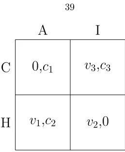
Figure 3.1: The Cheat-Audit Game

be to ignore that agent. Of course, it might be the case that auditing leads to catching a cheating agent, in which case the principal obtains a higher payoff than if he had chosen the costless action. By the same token, not auditing an honest agent is a better action for the principal, since auditing in this case expends auditing resources with no useful returns and — depending on how one sets up the model — can also incur a social cost in the form of the disutility or inconvenience that honest agents suffer because of auditing.

3.2.1

The Cheat-Audit Game

The example above is part of a large class of games that I call Cheat-Audit games. The payoffs of these game are as shown in Figure 3.1, with the principal being the column player. Each agent is considered a row player and has the row player’s payoffs. The actions available to an agent is to either be honest (action H) or cheat (action C). The principal either audits (action A) or ignores (action I) each agent. An agent’s payoffs satisfy 0 < v1 ≤v2< v3. To conserve notation, I will assume that v1 = v2, so that an agent is indifferent to auditing as long as he is honest. This assumption has no impact on any of the structural results I obtain. An agent is interested in

(49)

and no crime is committed, and the payoff to this outcome is normalized to zero. Similarly, an agent’s least preferred outcome is (C, A), and is also normalized to zero. Notice that the principal’s least preferred outcome, (C, I), is also the agent’s most preferred one.

Because of the large population assumption, the principal’s action consists of choosing a fraction 0≤α≤1 of the population to which he will apply actionA. I will call this fraction theaudit rate. The upper bound onαdoes not have to be equal to 1, but can instead be set to ¯αto indicate that it is not possible to audit the whole population. That the principal’s action consists of choosing a fraction to audit implicitly assumes anonymity of the agents in the population. In particular, the principal reacts to the distribution of play produced by the population, not the action of each individual.4 _{I formalize this in the following assumption.}

Assumption 3.2.1. (Anonymity) All members of the population in the Cheat-Audit game look the

same to the principal.

The diametric opposition of the principal’s and agents’ interests implies that the game has no pure strategy equilibria, as indeed can be checked from Figure 3.1 and the relationship between the various payoffs. In fact, similar to a game of matching pennies, the single-stage game possesses only a unique equilibrium in mixed strategies. Let the equilibrium audit rate and the fraction ofC

players in the fully rational setting be given byαN andxN, respectively. With the assumption that

v1=v2, it is straightforward to verify that

αN =

v3−v2

v3

; (3.1)

xN =

c2

c3+c2−c1

.

As mentioned, I consider an infinitely repeated setting where at each moment in time the game in Figure 3.1 is played. Discrete time and how it affects the results I obtain is discussed in Section 3.6. I will let the state of the system at time t be the fraction of the population taking action C 4_{One can think of scenarios where the identity of the player can be useful in the punishment phase, but not the}

(50)

at that time, and will denote this fraction by x(t). The principal’s choice of audit rate at timet is denoted byα(t). The large population assumption together with anonymity immediately imply the following result.

Proposition 3.2.2. The infinitely repeated Cheat-Audit game has a unique equilibrium in mixed

strategies. This equilibrium is the same as that of the stage game.

Proof. See Appendix.

The reason why Proposition 3.2.2 is true is that, because each agent is a negligible part of the continuum, any individual action has no effect on the distribution of play and thus no bearing on the future treatment of that agent.

Given a state x(t), audit rate α(t), and denoting the payoff to the principal at time t by

g(x(t), α(t)), the cost to the principal at timet is given by

g(x(t), α(t)) = c1α(t)x(t) +c2α(t)(1−x(t)) +c3(1−α(t))x(t)

= (c1−c2−c3)α(t)x(t) +c2α(t) +c3x(t), (3.2)

where the terms in the first equation in (3.2) correspond to the costs discussed above. The first term is the cost associated with catching offending agents, the second term represents the cost of auditing honest agents, and the last term is the cost of ignoring agents who were in fact playing actionC.

3.2.2

Learning Dynamics

(51)

Assumption 3.2.3. At the beginning of the horizon each strategy is played by a positive share in

the population, i.e., 0< x(0)<1.

Under this model, there are only two possible scenarios that can lead to switching strategies: an agent who obtained the outcome (C, A) considers changing his strategy if he meets an agent who playedH. Similarly, an agent who playedH considers changing his strategy toC if he meets an agent who obtained the outcome (C, I). The probabilities with which these changes in strategy occur depend on the differences in payoffs between agents, as well as a transmission factor k >0. One can think ofkas a ’speed of transmission’: the willingness of an agent to change their strategy when they meet someone with a better experience. Without loss of generality, I will assume that an agent who obtains payoff u switches to the strategy of an agent who obtained payoff v with probability max{0,v−_vu}. From Figure 3.1, the probability of switching in the first scenario is simply min{kv1−0

v1 =k,1}. The probability of switching in the second scenario is given by min{k

v3−v1

v3 ,1}. It

is important to stress that the way these probabilities are defined does not affect any structural results I obtain. Any scheme where the switching probabilities are proportional to the payoff differences, so that the share of strategies that perform better grows in the population, essentially leads to the same results. I will make the derivations less cumbersome and more general by assuming that switching in the first scenario happens with probabilitypand in the second scenario with probabilityq, and later substitute forp andq with the quantities above. Utilizing this notation, the fraction of switchers from C to H at any moment t is equal to the fraction of C players who were audited, α(t)x(t), multiplied by the probability of meeting an H player, which is 1−x(t), times the probability of switching p. Likewise, the fraction of switchers fromH to C is equal to the fraction ofH players, 1−x(t), who meet C players that were not audited, which is x(t)(1−α(t)), multiplied by the probabilityq. I can then write the dynamics of the system as a function ofx(t) andα(t)

˙

x(t) =f(x(t), α(t)) = q(1−α(t))x(t)(1−x(t))−pα(t)x(t)(1−x(t))

(52)

3.3

Myopic Principal

Before discussing the optimal policy for the principal, I consider the following question: what happens if the principal is myopic? Although there is strong reason to believe that the principal is more sophisticated than the population, there are many scenarios that encourage a short-sighted principal. A politician can pander to an electorate in the hopes of obtaining an immediate reward, or a corporate manager can make decisions with the goal of improving short-term gains as a response to pressure from investors. I will analyze such situations in this section by assuming that the principal learns in a myopic fashion and does this by adjusting his strategy after each round of the game in a similar manner to the population. This necessitates an assumption similar to Assumption 3.2.3.

Assumption 3.3.1. At the beginning of the horizon the princpal assigns positive weights to each

strategy, i.e.,0< α(0)<1.

Like the previous section, the cost of actionαisc1αx+c2α(1−x), while the cost to (1−α) is equal to the cost of those cheating agents who went away undetected, and is equal to c3(1−α)x. After each round, the principal observes the costs from both actionsH andI and adjusts the proportion by which they are played in the next round according to how well they did in the current round. Of course, the principal has no way of knowing whether the members of the population who were not audited were cheating or not. This is easily overcome by the large population assumption, since the fraction of the population that the principal audits identifies the fraction of cheaters in the population with probability one, and this fraction can then be used to estimate the costs incurred from not auditing.

(53)

oscillation. The following result gives a more precise description of the nature of interaction between the principal and the population under this setup.

Theorem 3.3.2. The fluctuations of the population ofCplayers and the audit rate of the principal

are periodic. The period depends on the values of the problem as well as the initial conditions. The

unique mixed equilibrium of (3.1) is a center of the dynamical system induced by the repeated play of the Cheat-Audit game.

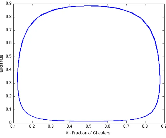
Informally, the equations with which the fraction ofCplayers and the audit rate evolve describe a dynamical system with a unique non-hyperbolic equilibrium. This equilibrium corresponds to the Nash equilibrium in (3.1), and — because the system has only two eigenvalues on the imaginary axis— is also a center of the system. This means that small perturbations push the system away from equilibrium. Being a center also implies that the path of any solution to the dynamical system is a closed orbit around the center. Thus, the system revisits each point in its evolution periodically. Figure 3.2 displays a phase portrait of the system, with the fraction of C players on thex-axis and the audit rate on they-axis. The closed orbit represents a solution that satisfies that following system

α(t)(1−α(t))[(c3+c2−c1)x(t)−c2) (3.4)

and

x(t)(1−x(t))[(v2−v3−v1)α(t) +v3−v2] (3.5)

(54)

to extreme auditing of the population that eventually drives the majority to playH again, and the cycle repeats. As I discuss in Section 3.6, this cyclical nature can be observed in various real-world phenomena that correspond to the Cheat-Audit game.

3.3.1

Average Cheating and Audit Rates

It is natural to ask how the scenario analyzed above differs from the rational case. It turns out that if the game is played long enough, then the players’ actions, averaged over time, are equal to the corresponding values in the fully rational setting. This accentuates the early discussion about replicator dynamics: even though they are following very simple rules, both the principal and the agents are able to approximate the behavior of their rational counterparts. In particular, the fraction of C players and the principal’s audit rate over any period are the same as those obtained in the mixed equilibrium solution given by (3.1). The following result formalizes this fact.

Theorem 3.3.3. The average audit rate of the principal and the average fraction of cheaters over

any period are the same as the corresponding Nash equilibrium values.

Having shown that the outcome of the game between the myopic principal and the population is close to the fully rational outcome, I proceed to show how a forward-looking principal can improve on the results of the fully rational setting.

3.4

Forward-Looking Principal

(55)

Figure 3.2: Phase Portrait of Cheating and Auditing Activity

3.4.1

Objective

The principal’s problem is the following: Given the different values in Figure 3.1 and the learning dynamics, the principal is interested in minimizing the long-run discounted cost. This long-run cost is the discounted sum of all costs accrued from playing the game over time. Recall that the payoff at time t is given by (3.2) and the equation of motion of the population by (3.3). The principal’s problem can then be written as

min

α(t)

R∞

0 e

−rt₍₍_c

1−c2−c3)α(t)x(t) +c2α(t) +c3x(t))dt (3.6) s.t. x˙(t) =x(t)(1−x(t))(q−α(t)(q+p))

0≤α(t)≤1

(56)

(57)

(58)

(59)

Theorem 3.4.3. There is a valuex¯such that the optimal policy audits everybody wheneverx(t)>x¯

and does nothing whenx(t)<x. If¯ x(t) = ¯xthen the optimal policy setsα∗(t) = _p₊q_q and the system stays in this state indefinitely.

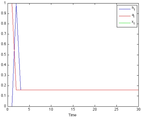
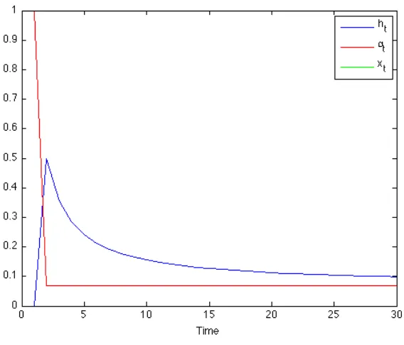
Theorem 3.4.3 indicates that, depending on a threshold value, the optimal solution either audits indiscriminately or does nothing. If the system hits the value |barx, then the system audits at a constant rate. The structure of the optimal policy then is quite different from the myopic principal case, where the principal’s strategy oscillates continuously. As I discuss in Section 3.6, the optimal policy can oscillate too, as a result of considering the model in discrete time.

3.5

Comparison With The Nash Equilibrium

How does the solution for the class of games considered here fare under the forward-looking principal in comparison to the fully rational Nash equilibrium outcome? I have already discussed in Section 3.2.1 and in Theorem 3.2.2 that the (fully rational) repeated game possesses a unique equilibrium in mixed strategies, given by (3.1). As I have shown in Theorem 3.3.2, this equilibrium is also acenter

of the repeated behavioral game. This means that, under the replicator assumption, there exists a strategy such that if the game is played long enough, the fraction with which each action is played is the same as the corresponding fraction in the Nash equilibrium, i.e., the principal can implement the Nash outcome in the behavioral setting, if he so desires. However, the optimal solution that I obtained in Section 3.4 is not the Nash equilibrium, indicating that the Nash solution is dominated by the policy in Theorem 3.4.3. Furthermore, as I show below, as soon as the game reaches steady state, the optimal policy involves less auditing than the Nash solution. Because of this, the Nash solution never coincides with the policy in Theorem 3.4.3, so that the optimal solution always gives a strictly better outcome for the principal while at the same time reducing the amount of auditing required.

(60)

a principal can obtain when facing a behavioral population. The principal is able to both perform less auditing and, if concerned enough about the future, keep the fraction ofCplayers close to zero.

Theorem 3.5.1. The steady-state audit rate in the behavioral setting is strictly less than the Nash

audit rate. Letr >0 be a discount factor, thenlimr→0¯x= 0, i.e., as the principal cares more about

the future, the fraction ofC players is driven close to zero. This contrasts with the Nash fraction of

C playersxN, which is insensitive to the effect of discounting.

This result highlights the stark difference between the behavioral and rational settings. Discounting has no bearing on the outcome in the rational case since, as Theorem 3.2.2 shows, the principal cannot influence the future actions of the population. Furthermore, from Theorem 3.3.3, the outcomes in the behavioral setting are close to the Nash solution when the principal responds myopically. By taking the future into account however, the principal is able to obtain outcomes that were not possible under these other scenarios. As I discuss in the next section, the results in Theorems 3.3.2 and 3.4.3 are widely observed in practice.

3.6

Examples

Eeckhout, Persico, and Todd (2010) define crackdowns as intermittent periods of high-intensity mon-itoring. Crackdown cycles occur when these periods are interwoven with periods of lax enforcement. There is a wealth of examples of this phenomenon. Di Tella and Schargrodsky (2003) study crack-downs on corruption in hospitals in Buenos Aires, Lui (1986) describes crackcrack-downs on corruption in China, the Recording Industry Association of America (RIAA) utilizes crackdowns to combat illegal file sharing, and police in Belgium intermittently crack down on speeders. I discuss some of these examples and show how they relate to the results of the previous sections.

(61)

years, ending in June of 1952. The campaign was characterized by a highly intensive effort that managed to reduce crime from 500,000 cases in 1950 to an average of 290,000 cases over the following 15 years. Thesan fanwas not just characterized by severe punishments, but also by extremely high auditing activity, and during the crackdown period crime steadily declined to very low rates. As the cycle in Figure 3.2 predicts, the post-crackdown period was characterized by low crime ratesandlow monitoring activity, and has nowadays come to be known as ’the golden age of honesty’ in China6, where as Lui puts it, ’the Chinese government did not spend any significant amount of resources on auditing’. Eventually though, corruption started to increase again, and the government cracked down on both corruption and dissidence in the middle of the 1960s. The pattern was then repeated as the decrease in monitoring after the second crackdown led to a rise in corruption levels, which by 1979 were getting out of control. This led to a third crackdown that started in 1982 and lasted for more than three years.

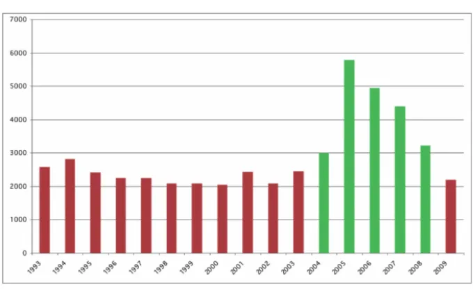
A more recent example is how the RIAA and the Motion Picture Association of America (MPAA) fight online piracy and illegal file sharing. Figure 3.3 shows copyright infringement lawsuits in the United States over the period 1993–2009.7 _{The beginning of the millennium witnessed a huge} increase in the number of file sharers, where platforms like Napster had a record 26 million users at one point. The percentage of internet users who were also illegal file sharers continued to grow, hitting a high of 29% of all US internet users.8 _{As one can see in the figure, the RIAA responded} with a severe crackdown that started around 2004 and lasted for five years. During the crackdown, the amount of infringement lawsuits tripled. Most of these lawsuits targeted anonymous, ’John Doe’ defendants. The crackdowns resulted in a drop in the percentage of file sharers from 29% to 14%, with the number stabilizing somewhere around 18%.9 _{In 2008, the RIAA announced that it has} stopped its mass-lawsuit practice but that it will continue to sue users at a lesser rate. Although in 2010 it is early to tell, this pattern bears a striking resemblance to the policy in Theorem 3.4.3, where a severe crackdown brings the fraction of offenders down to a certain level, after which auditing

6_{Lui (1986)}

7_{Source: Administrative Office Of The Courts}

8_{Source: PEW Internet and American Life Project Data Memo}

(62)

continues at a lower rate. Of course, there are many factors that go into a campaign like the one launched by the RIAA, including publicity of, and backlash against, the lawsuits, but the overall agreement of the pattern with the results obtained in this chapter suggests that the core driving factors are captured by the model.

(63)

observations are explained by the model in this chapter. The recurrence of the crackdowns takes place as the police tries to bring the fraction of speeders to an optimal level, and since the evolution of the population of speeders can be determined from the current state and future controls of the system, the time at which such a crackdown would be necessary can be determined in advance as well.

3.7

Other Applications

3.7.1

Equilibrium Selection and Technology Adoption

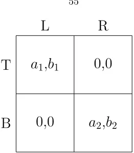
The framework I use in this chapter can also be used as a device for equilibrium selection. The fact that a game may possess multiple equilibria makes it more difficult to design mechanisms that select for a particular equilibrium with certain desired outcomes. Balcan, Blum, and Mansour (2009) consider the problem of moving a population from one equilibrium to another one with more socially desirable properties. Their framework uses public advertisement as a means to influence decisions in the rational agent population, and they analyze the effectiveness of this method even when only a small fraction of the population follows the advertisement. In many cases, the proposed method fails to move the population between equilibria. For coordination games like the one in Figure 3.4, I show how a principal can steer the population towards an equilibrium that is worse for them but is beneficial for the principal.

(64)

L

R

T

B

a

1

,

b

1

0,0

a

2

,

b

2

Figure 3.4: Coordination Game

The situation described above is depicted in the coordination game in Figure 3.4, with the principal being the column player. Assume a1 < a2 and b1 > b2, so that the principal’s preferred outcome is (T, L), while the population prefers outcome (B, R). Similar to the setup in Section 4.2, I denote the fraction with which the principal plays action Lat time t byα(t), while the fraction of the population playing L is denoted by x(t). One can interpret αas the fraction of the firm’s resources that it devotes to sustaining techology L and 1−x(t) as the fraction sticking with the old technology. By Assumption 3.2.3, the share of the population playing either strategy at the beginning of the horizon is positive. This corresponds to the fact that the new technology has early adopters. The question then is whether the principal can facilitate the migration of the population towards an equilibrium that is more desirable for him, which in Figure 3.4 corresponds to equilibrium (T, L).

As before, I will first consider the outcome of this interaction when the principal adopts a myopic approach. For scenarios like the one discussed above, it is reasonable to expect that the system starts somewhere close to the (B, R) equilibrium, where most of the population has still not adopted the new technology and the firm still offers extensive support for the old technology. Under this setting, a myopic principal cannot move the population near equilibrium (T, L). In fact, the following result shows that a myopic principal gets stuck at the (B, R) equilibrium forever.

Theorem 3.7.1. If the system starts in an interior state wherex(0)> b1

b1+b2 andα(0)>

a2

a1+a2, then

(65)

(66)

for the old product, leading the population to migrate towards using the new one.10 _{As the principal} cares more about the future, it is willing to sustain some ’transitory costs’, the costs that it incurs as a result of unsatisfied customers, in order to accumulate later gains. In this sense the optimal policy is similar to the policy in the Cheat-Audit game: crackdown on the population in the optimal strategy incurs costs from auditing H players, or not auditing anyone incurs costs from lettingC

players go undetected. These costs are, agai