PROOF THAT P 6=NP∗
1
JAMELL IVAN SAMUELS†
2
Abstract. The question does P = NP has confounded mathematicians and computer scientists
3
alike for over 50 years and although there is an almost unanimous agreement that it in fact does not,
4
there still is no absolute proof. In this paper, I attempt to prove to that P does not equal NP.
5
Key words. NP, P, Computational Complexity
6
AMS subject classifications. 68Q12, 68Q17
7
1. Introduction.
8
In 1971 Stephen Cook [1] proposed a fundamental question to the theory of computer 9
science. The question does NP = P has serious ramifications across a broad range of 10
subjects from cryptography to DNA synthesis and a solution to this problem has been 11
deemed worthy of a Millennium Prize. In this paper I establish the proof through the 12
use of basic fundamentals. 13
2. Counting.
14
In mathematics the two basic operations are counting and totalling. 15
Definition 2.1. 16
Counting is the acting out of a method using a unit measure. Example there are a
17
hive of bees, I count the bees using my unit measure| as||||||.
18
Definition 2.2. 19
Totalling is the explicit use of number to sum a count, I sum my count||||||using my
20
numerical system1,2,3,4.... as6.
21
Counting and totalling inhabit a region named the Method SpaceM, which is an 22
area used to categorise and derive operations. 23
Definition 2.3. A Method M is any operation or process used to solve a problem.
24
In the Method Space, methods are represented as M(current operation, next variable),
25
wheren ∀Randi ∀R.
26
Definition 2.4 (Limit of Counting to 0). 27
The limit of counting to 0M(n, i) limi→0M(1,0) 28
The limit of totalling to 0M(n+ii, ii+1) limi→0M(n,0) 29
Definition 2.5 (Limit of Counting to∞). 30
The limit of counting to infinityM(n, i) limi→∞M(1,1) 31
The limit of totalling to infinityM(n+ii, ii+1) limi→∞M(∞,∞) 32
Using the method of slopes to measure the difference between counting and to-33
talling . 34
(2.1) d∆T
d∆C =
M(∞,∞)−M(n,0)
M(1,1)−M(1,0) =
M(∞,∞)
M(0,1) ≡
(∞,∞) (0,1) 35
Dividing to resolve this equation you obtain. 36
(2.2) (1,∞)
37
∗Submitted to the editors 02/07/2020.
†Imperial College London, London, ([email protected],http://www.researchgate.com/∼ddoe/).
Thereby establishing 0 as a non countable number. 38
3. Checking and Solving.
39
Definition 3.1. Checking is the process where you assure that the solution you
40
have gained is valid.
41
Definition 3.2. Solving is the method used to acquire a solution. 42
Lemma 3.3. Your best solving method can not run faster than your best checking 43
method. Solving lim−−−−−→M ethod Checking
44
4. Probability.
45
Probability can be stated as the likelihood that an event will occur. It is counted as 46
the number of times an event will occur given the total number of possible events. Any 47
probability outside the boundaries of [0,1] does not exist on the probability plane and 48
therefore can only be interpreted for it’s meaning rather than stated as an absolute 49
definition of chance. 50
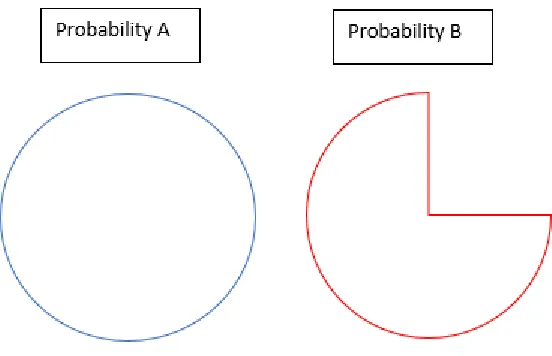
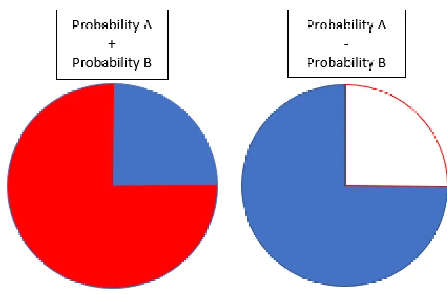
4.1. Planes and Cylinders of Probability.
51
Probabilities must remain on the same plane and in truth they can only be added or 52
subtracted. The use of multiplication can be considered the resolution of a stack of 53
probabilities (and therefore multiple events) that exist on separate planes which you 54
have resolved to one. Therefore we can define a probability plane or cylinder as. 55
Fig. 2.Probability Cylinder.
• A probability plane is the area in which a probability exists or acts upon. 56
Probabilities may exist on separate planes, but they must be resolved to act 57
on one. 58
• A probability cylinder is a stack of multiple planes, a cylinder must be resolved 59
to act on one plane to calculate the probability of the single event. 60
4.2. The Fundamental Probability - Derivation of Given.
61
The most fundamental probability to calculate is the probability that event(B) is not 62
going to happen given that event(A) has or is going to happen. All other probabilities 63
that can be calculated, fundamentally rely on this and although can be calculated in 64
other ways, risk losing the information contained within. Henceforth we are going to 65
state the probabilities in the order that they are calculated. 66
(4.1) P(!B|A) =P(A)−P(B) 67
(4.2) P(B|A) =P(A)−P(!B|A) 68
4.3. A note on Circular Logic.
69
The statement P(B|A) = P(A)−P(A|!B) is self refuting and is therefore contra-70
dictory. Probabilities as a matter of fact can not be self proving or self refuting as 71
both are a form of circular logic. It is also not possible to circumvent this by stating 72
P(B|A) =P(A)−P(!B|A), because a ’not’ case, not derived from an initial ’is’ case, 73
technically comes from a separate ’world’ of probability. Example 74
(4.3) P(A) = 1; P(B) =1
2 75
76
P(A) +P(B) =3 2 77
78
P(!A) +P(!B) =1 2 79
It can be seen that the two sums are distinctly different and therefore they can 80
not be considered to come from the same case. 81
4.4. Simultaneous Occurrences.
82
Probabilities must exist on a single plane and as a single event. Any event with more 83
than one possible outcome can be considered a simultaneous event. When resolving 84
multiple events to a single plane or in a single plane, the probabilities must be fully 85
counted to not lose or create inconsistencies in the information contained. 86
4.4.1. Probability of∧.
87
If you recall the standard probability definition of ”and” isP(A∧B) =P(A)×P(B). 88
P(A) = 1; P(B) =1 9 89
90
1×1 9 =
1 9 91
Therefore. 92
P(A∧B) =P(B) 93
And you can henceforth state that the eventP(A∧B) is not dependent onP(A). The 94
same argument can also be made forP(A|B). And ergo P(A∧B) is fundamentally 95
contradictory. This can be stated because the use of multiplication is the loss of 96
information. For example. [5 + 5 + 5 + 5 + 5] contains more information than 5×5. 97
It is therefore better to state that P(A∧B) =P(A|B)×P(B|A). And to treat all 98
P(A∧B) =
P(A|B)
P(B|A) (4.4)
100 101
4.4.2. Probability of∨.
102
Although the probability of (A∨B) can be considered a fundamental probability as 103
it can be calculated as P(A) +P(B), it is actually one of the derived probabilities 104
as it has more than one possible outcome and therefore must be resolved as a single 105
event. 106
P(!A∨!B) =
P(!A|B)
P(!B|A) (4.5)
107 108
P(!A∨!B) =P(A∧B) +P(!A∧!B) (4.6)
109 110
P(A∨B) = 1−P(!A∨!B) (4.7)
111 112
5. Non-Polynomial Time Problems.
113
Any Non-Polynomial problem is the result of two distinct and independent variables. 114
I shall refer to these as the value and the order. 115
• Valuevis the property of a variable that makes it distinct. 116
• Ordero is the particular arrangement of properties in manner that is trans-117
ferable to a base 1 count. 118
An example of this is Sudoku, where the values are placed in a particular order 119
to solve the problem. Any problemS which can be described in this manner is what 120
we shall consider a Non-Polynomial problem for the sake of this argument. 121
Definition 5.1. Polynomial Problems 122
S =f(v, o) 123
o=f(v) 124
S =f(v) 125
P(S) =P(A) 126
127
Definition 5.2. Non-Polynomial Problems 128
S=f(v, o) 129
o6=f(v) 130
S6=f(v) 131
P(S) =P(A|!B) 132
133
5.1. Proof the Problem is exponential.
134
In the previous section, it was stated that non-polynomial problems are dependent 135
on v and o. When solving a non-polynomial problem it is typical to say a solution 136
is found when both events A and B occur,P(A∧B). However in truth, a solution 137
is found when given event A, B has occurred which can only be written as P(B|A). 138
However, when deriving a solution P(A|!B) must be used as P(A|B) as previously 139
5.1.1. P(!B|A). We are now going to derive the algorithm as given event A has 141
occurred, event B will not happen. Where A is the probability that the order is 142
correctB is the probability the value was correct and nis length of the problem i.e. 143
the number of possible solutions . 144
P(A) = 1 The order is always assumed correct
(5.1) 145
P(B) = 1
nThe value is assumed as typical to be
1 n
146
P(A|!B)Algorithm=P(A)−P(B) 147
148
• For an algorithm to be correct the probability of finding a solution must equal 149
1. 150
P(A|!B)Algorithm = 1.
(5.2) 151 152
• Forn2required solutions the probability of finding the correct solution is. 153
P(A|!B)Algorithm= (P(A)−P(B))n2= 1n2 (5.3)
154 155
Using the binomial identity 156 n2 X k n2 k
An2−kBk= 1.
(5.4) 157 158
• Where k represents a single step i and is equal to 1 159
• This can be expanded as 160
n2
0
An2B0−
n2−k
k
Bk+
n2−2k
2k
B2k...+
0
n2k
B2n2k
(5.5) 161 162
• AsB is applied as a negative, every (k+ 1)thstep is impossible and therefore 163
incalculable. We must therefore increase the total length of the algorithm to 164
2n2 165
2n2
0
A2n2B0+
2n2−2k
2k
B2k...+
0
2n2k
B2n2k
(5.6) 166 167
• SubstitutingBk= 1
n k 168
2n2
0
An2
1
n
0
+
2n2−2k
2k 1 n 2k ...+ 0
2n2k
1
n
2n2k
(5.7) 169 170
• As previously stated, you can not count 0. And therefore the expression for 171
the algorithm becomes 172
2n2−2k
2k
1
n
2k
+
2n2−4k
4k 1 n 4k ...+ 0
2n2k
1
n
2n2k
= 1.
5.1.2. Limit Of Probability.
175
If we are to assume that the solution we are checking is correct, the probability that 176
the value and the order are correct are both 1. 177
P(A)Check= 1 (5.9)
178
P(B)Check= 1 (5.10)
179
P(A∧B)Check= 1 (5.11)
180
P(A|B)Check= 1 (5.12)
181 182
A property of a check is that it is self proving. So given the nature of the problem 183
the probability of the check can be defined asP(A|B). The probability of a check can 184
also be stated to beP(A∧B) as an efficient polynomial checking algorithm will only 185
total. Removing the co-efficients from the previously stated algorithm and taking 186
the pure calculation, synonymous to reducing the algorithm from a non-deterministic 187
algorithm to a deterministic algorithm. 188
P(A|!B)Algorithm= 1 n 2 + 1 n 4 + 1 n 6 +... 1 n
2n2
= 1 (5.13)
189 190
The limit of the sum is. 191
ΣP(A|!B)Algorithm →lim 1.
(5.14) 192
193
And therefore, for non-polynomial problems, as the probability that any poly-194
nomial algorithm cam correctly solve the problem can never equal 1, there is no 195
deterministic algorithm that can solve the problem in P time. 196
5.1.3. Proof of Exponential Nature.
197
Proof. Recalling that the relationship betweenP(A),P(B) andnis 198
199
Πn2
k=1P(A)n
2−k
P(B)k= 1
n
P2k
wherek=
n2
1 200
As the left side is checking, let it be said that P(A) =P(B) = 1 201
1 = 1
n
Pn
2 1 2k
202
ln|1|=−Pn2
1 2kln|n| 203
0 =−Pn2
1 2kln|n| 204
0 = −
Pn2
1 2k
n derivative 205
e0=e
−Pn2
1 2k
n
206
1 =e− Pn2
1 2k
n
207
Thereby proving that the problem is naturally exponential. This expression can be 208
calculated as, 209
1 =−1. 210
And as the modulus of 1 = | −1| we can conclude the problem is correctly solved, 211
however, as−16= 1 we can also conclude thatN P 6=P. 212
5.2. The Argument of Intent.
214
P(!B|A) represents an algorithm with the intention of getting it wrong/’can be said 215
to be not knowing’. However, by some miracle it manages to get it right, if only once, 216
as it’s limit approaches 1. However, P(B|A) which is equal to (1−8
9) can never get 217
it right. As the algorithm that intends to get it right, can not get it right, and the 218
algorithm that intends to get it wrong can, we can therefore state that there is no 219
single intentional method that can solve this problem and we can therefore conclude 220
that no efficient polynomial solution exists. 221
222
5.3. Upper Bound.
223
As previously stated inLemma3.3, the limit for solving is checking. 224
Solving lim−−−−−→M ethod Checking (5.15)
225 226
e
−Pn2
1 2k
n lim−−−−−→M ethod 1
227 228
2n2e
−Pn2
1 2k
n lim−−−−−→M ethod 2n2
229
And therefore we can state that the Upper Bound is equal to 230
2n2e
−Pn2
1 2k
n .
231
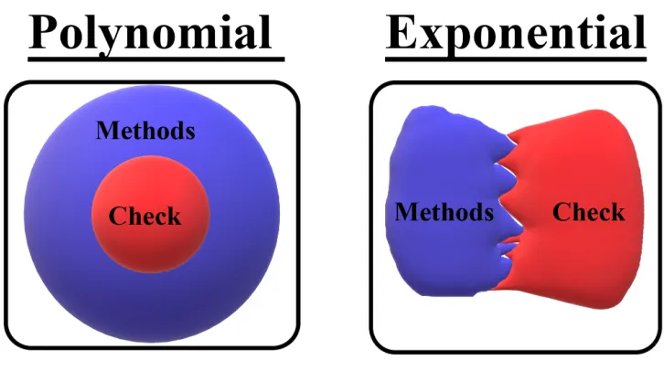
Fig. 4.’Method Space’ for polynomial and non-polynomial problems.
Acknowledgements. Thank you to Sergei Chernyshenko for dissecting an ear-232
lier copy of my work. 233
REFERENCES
234
[1] Cook. A.S, ”The P versus NP Problem”Clay Mathematics,