225
Volume LIX 23 Number 7, 2011
ELASTICITY OF DEMAND OF
THE CZECH CONSUMER
J. Luňáček, V. Feldbabel
Received: August 31, 2011
Abstract
LUŇÁČEK, J., FELDBABEL, V.: Elasticity of demand of the Czech consumer. Acta univ. agric. et silvic. Mendel. Brun., 2011, LIX, No. 7, pp. 225–236
The price elasticity of demand enables to set the real “correct price” to the seller guaranteeing the highest income. Despite the fact that the price elasticity of demand is very important in the economic practice, no work that would deal with it in greater details seems to be elaborated till now. The available sources show practically only and exclusively coeffi cients of the price elasticity of demand in the United States. These coeffi cients can naturally be utilized, but for certain goods only (e.g. salt, etc.), where the demand is the same irrespectively of where we fi nd ourselves globally. There are certain products and services where the demand is determined by the socio-cultural aspects following from certain traditions of the country in question. The values established for conditions of the Czech Republic are certainly available nowadays, but with respect to expensiveness and scope of these researches we cannot consider them comparable with the results from the USA.
Objective of this paper is to draw curves of demand of 20 commonly used commodities in the Czech Republic and to determine coeffi cients of the price elasticity of demand a erwards, from which the basic recommendations for their sellers will follow. In light of the facts above comparison of these coeffi cients with the data from the USA would be very interesting to be able to create the picture about dissimilarities in demand of the average Czech and American consumer.
demand, elasticity of demand, statistics evaluation, questionnaire investigation, modelling
Economics in practical use should serve for understanding of a deeper relationship between individual phenomena on the market. At the beginning of this research it is necessary to realize that in case of each market transaction there must be a buyer and the seller who − if he wants to succeed − must unconditionally understand how the market transaction works on the demand side and what are the main determinants of the demand. The theory of demand deals with this assignment within the scope of the microeconomics.
Unfortunately it is not enough, though the theory of demand enables to understand the customer’s behaviour, but would not be useful explicitly by itself for us, the sellers. We would assume that with the rising product price the demanded quantity would fall naturally, but the most interesting fact for us should be, how the demand will change precisely.
To fi nd a satisfactory answer to the question above, the microeconomics has a very eff ective instrument in the form of the price elasticity of demand. It is able to describe the said consumers’ reaction to the changes best of all and, moreover, the well understood price elasticity of demand refutes the widespread idea among the laymen that the sellers off er their goods “for the highest possible price”. By selling for the highest possible prices they would in fact harm themselves in many cases, because headless price increase would result in reduction of their receipts ultimately.
according to our opinion it represents a reasonable compromise between miscellaneous approaches to data collection from individual respondents. It is possible that other methods (e.g. interview) could enable easier aff ection and directing of the respondent so that his/her answers may not steer away from the context of established facts, but the questionnaire research is much more advantageous from the point of time consumption. On the other side it is necessary to point out the no type of the public opinion research in the fi eld of demand should be overestimated, because the absolutely perfect prediction of demand of the individual is principally not possible, as we are always speaking about the attempt to estimate consumer’s behaviour as reaction to certain price impulses, which, contrary to the „ceteris paribus“ rule, are the integral part of a certain complex of decisions following not only from the buyer’s eff ort to maximize his/her profi t, but also from the buyer’s reaction to certain fashion and social trends and conventions, which can change relatively quickly in time.
The questionnaire research of the market demand is quite adequate with respect to its possibilities; possible deviations of the established values from the real ones are only the matter of data processing through a suitable statistical apparatus which is able to characterize such deviations exactly. To reach the least possible statistical error, the questionnaires were selected thoroughly prior to loading the data into the selective set. The selection consisted in elimination of the questionnaires fi lled in contrary to the introductory instruction, and/or the questionnaires that presented unreal values of consumption, both with respect to fi nancial possibilities of the respondent and factual possibility of consumption of the shown goods quantities. Such data, when incorporated into statistical calculations, would become the source of the so called gross errors and could misrepresent the obtained results explicitly.
Description of questionnaire
Our research was focused on determination of the demand curves of 20 commodities and structure, content and formal appearance of the questionnaire was adapted to this purpose. In conformity with the basic rules of creation of the questionnaires the respondent was familiarized in the short introductory part with importance and objectives of the questionnaire research and was assured about anonymous character of the whole research. The respondent was also notifi ed that consumption of his family as the elementary social unit created by a certain number of respondents, the family having a certain fi nancial budget, is the subject matter of the study; and the important „ceteris paribus“ condition was clarifi ed as well.
In the next part the respondents indicated number of members of their household and fi lled in the monthly demanded quality of the commodity in relevant units for a certain price broken down
into several price zones into the pre-printed tables. The term of one month has been chosen, because the fi nal part contains the question concerning the net family income per month. Only in case of the goods, consumption of which per month is so low that estimate of the monthly consumption would be diffi cult for the respondents, the time period has been modifi ed to one year.
The average income of one member of the household and the average income falling on one respondent a erwards can be determined very easily from the indication concerning the net income of the household. It is necessary to point out here that this income is quite naturally broken down even into the non-earning members of the household (i.e. children, unemployed persons, etc.), because for existential reasons even the non-earning persons must satisfy their basic and other needs. From the words above it follows that it is advisable to calculate the average earning falling on each member of the family, incl. the children, as the theoretical sum, which is available for each member of the household for satisfaction of his/her needs, though this ratio can in fact be diff erent to a certain degree.
The price zones applied for individual goods commodities have been chosen, based on two principles. The fi rst principle consisted in the requirement that the “common price” of the given goods must lie in the average zone of the price range, with subsequent price range passing into the zones of extremely low and extremely high prices. The second principle concerned the price zone width; it was chosen so that the points of consumer demand may lie in uniform spacing along the demand curve, thus enabling more precise analytical processing and estimate of the course of the demand curves themselves.
Determination of the selective set size
The data obtained from the questionnaire research will be processed, using the elementary statistical methods and therefore, should the obtained data be relevant adequately, the optimum size of the selective set must be determined, because this set will represent opinions of the remaining consumers creating the basic statistical set (e.g. inhabitants of the Czech Republic). This objective can again be reached by applying the correct procedure of the mathematical statistics.
• Share of the really examined selective units must not depend on the size of the selective set. In practice large sets are so demanding from the organizational point of view, that the percentage of persons caught and engaged for cooperation falls with their scope as a rule.
• No non-selective, systematic error, caused for instance by unclear understanding of certain questions, unwillingness to release certain data, etc., may exist.
Simple random selection with repetition and/ or without repetition is most frequently used for creation of the selective set of requested features identifi ed above. It is the direct selection of the respondents from the unsorted basic set and each member of the selective set has the same possibility to be addressed randomly. As we are speaking about the random selection with repetition (and/or without repetition) each respondent can be (and/or cannot be) inquired repeatedly.
It is necessary to point out that if the basic set comprises a high number of units, then diff erences between these types of selections are negligible.
If T is the estimated characteristics of the basic set and if is its estimate following from the data of the selective set, then |T − | is named error of the estimate and the ratio |T - |/T is the relative error of the estimate. Should the error of the estimate equal max. to the fi gure Δ, then this value is named the permitted error of the estimate. Should the relative error of the estimate equal max. to the fi gure , we are speaking about the relative permitted error of the estimate. The relative errors of the estimate are expressed usually in per cents. Sizes of the error or the relative error are the basic indicators of accuracy of the research and the public opinion researches usually determine the permitted relative error of 5 % (Pecáková et al., 1998; Řezanková, 2007).
When estimating features of the basic set by applying the data from the selective set, you can never be sure that error of the estimate will equal max. to the fi gure Δ and/or that estimate of the relative error of measurement will equal max to the fi gure and therefore we can only request these error claims to be probable adequately. This is expressed by the probability designated 1 − and named reliability coeffi cient or reliability coeffi cient of the estimate (e.g. for 1 − = 0.90 we are speaking about 90 % reliability). Whilst in technical and highly exact fi elds the reliability coeffi cient is requested higher than 95 %, in case of the public opinion researches the reliability coeffi cient is usually lower with respect to a high variability of answers.
The simple random selection without repetition was used for the questionnaire research. The following formula is valid for the scope of the selective set, that would guarantee reach of the requested values of error and relative error with the given probability:
2 2 1
2
2 2 2
1 1 2
1
u
N
n
N
u
, (1)where n is the scope of the selective set, is the standard deviation and N is the scope of the basic set. Number 1 1
2
u
is quantile of the standardized normal
distribution depending on the chosen reliability 1 – (for the 90 % reliability coeffi cient value of this quantile reaches 1.645) (Hindls, 2007). As the demand curves, which elasticity of certain kinds of goods is determined from, have been elaborated for the basic set representing population of the Czech Republic, it is the adequately large set enabling to utilize the relations for calculation of the size of the selective set created by the simple random selection with repetition, because the results are comparable. The following is valid:
2 2 1 2 2
u
n
, (2)if I extend the fraction by the arithmetic mean of the monitored characteristics x, I will receive the following: 2 2 1 2 2
u
V
n
, (3)where V is the variation coeffi cient defi ned as the quotient of the standard deviation and the average value. From the formula it follows clearly that the higher the requested estimate reliability and the lower the requested permitted error, the higher is the scope of the selective set. It is also evident that under otherwise identical conditions size of the selective set depends on variability of distribution of the monitored numerical variable in the basic set, i.e. the higher the variability of these values, the higher the selective set must be and vice versa. The literature sources (Hindls, 2007) show that in case of the numerical variables monitored in the public opinion researches and in the market researches, values of the variation coeffi cient most frequently range from 0.3 to 1.0.
If relevant calculation is performed, where the relative error value is requested at the level of 5 %, reliability at the level of 90 % and, if assumed, that the variation coeffi cient is 0.65 (the centre of the interval of usual values), the following value will be obtained for the scope of the selective set:
2 2
2
1,645
0,65
457
0,05
i.e. if I want to reach the parameters of research as above, I have to address at least 457 respondents within the scope of the simple random selection.
Methodology of statistical processing of the obtained data
When processing the questionnaire data for determination of the demand curves, we face the problem what statistical apparatus to choose to reach the relevant results that would refl ect the fact, which we try to estimate empirically, with adequately high weight. Accuracy of approaching to the estimated fact (which is de facto unknown) by the established data is expressed by the statistical error or by the intervals of reliability. From individual sources it follows that the method of data processing, when the set of points in the P/Q graphs is completed by the curve (using the regression analysis) where individual points express the aggregated demand at the given price, is the standard method of data processing when determining the demand curves and the curves of elasticity. As this method is standard, there is no sense to analyze it in greater details in this part. Though the methods of regression analysis are well known and used, the authors think that another method is more suitable for processing the data obtained from the questionnaire research.
Interleaving the established points by a curve is the basic problem. These items will lie close to the curve, i.e. the deviations are too small, which fact could lead to illusion of a good and precise result of the empiric research. This fact can be caused by the fact that the preceding methodology does not consider variability of answers of individual respondents that has material impact on accuracy of determination of the average demand and thus the elasticity.
If the statistic deviation is determined, based on the average ”distance of points” of the overall or average demand from the approximation curve, then the deviation necessarily depends on the type of the curve used for approximation. It means that this method of error determines the degree, how precise is the chosen approximation curve, which for instance in case of interpolation (the curve passes through all points) leads to the zero deviation, but does not say much about accuracy of the empirically obtained data. Consequently, even if the deviation is minimum, course of such curve does not need to copy the real curve of demand of the basic statistical set which we try to estimate by the methods above.
Underestimate of the deviation calculated by the method above could easily lead to the unpleasant fact that in case of realization of another random selection from he basic set we receive point
estimates of the mean values of the demanded quantity and elasticity that would lie out of the interval determined by the deviation calculated from the fi rst selective set.
When processing the questionnaires, we have caught accuracy of measurements following from diversity of answers of individual respondents by calculation of the mean quadratic error Sx determining the reliability interval round the arithmetic mean. The real mean value of the measured variable lies with the probability P = - 1 in the interval x − Δx; x + Δx, where
( )
xx t f S
.Sx ... is standard deviation of the arithmetic mean of the selective set
t(f) ... is coeffi cient of the Student’s distribution,
... is the chosen degree of importance (risk), f = n −1 .is the number of degrees of freedom, n ...is the number of measurements.
In our research the degree of importance of 68 % is considered, which corresponds to the value of the coeffi cient of the Student’s distribution 1. In this case the following formula is valid for the mean quadratic error (Hindls, 2007):
2
1
( )
1
n
i i x
x x
x S
n n
.
By the questionnaire research we have established the selective set, the scope of which corresponds to the n respondents who have fi lled their individual demanded quantity of the given commodity in individual tables of the questionnaire in several fi xed price ranges, see the sample below (Tab. I).
From the table fi lled in by the k respondent for the j kind of goods the mean value Pji of the price zone restricted by the limit values P’jiand Pji’’will be determined. Qkji is the corresponding demanded quantity within the given price zone and time period (one month as a rule as clarifi ed above).
From the data of all respondents we can calculate the overall demand of the selective set for the j goods in the i price zone by using the formula below:
Cji kji
k
Q
Q (5)and even the average demanded quantity of the j kind of goods at the i price value a erwards, by applying the formula:
I: Questionnaire table for determination of the demand of the k-respondent for the j-goods (our own processing)
kji Cji k ji
Q
Q
Q
n
n
. (6)This average value represents (from the statistical point of view) the point estimate of the mean value of the demand of the basic set.
The average net income falling on one respondent is another information that can be determined from the questionnaire data, see the formula below:
k C k
I
I
I
n
n
, (7)where IC is the overall net income of the selective set and Ik is the net income of the k respondent.
The next step accommodates calculation of the mean quadratic error of the average demand Qjifor the j kind of goods at the i price level by applying the well known formula/relation:
2 1 1 ji n ji kji k Q Q Q S n n
. (8)All calculated data will be put down into the table, see the sample below (Tab. II).
The following formula will be used for calculation of elasticity:
22 1
1: 2
22 1
1: 2
D
Q
Q
P
P
E
Q
Q
P
P
. (9)During practical calculation of the price elasticity corresponding relative changes of the demanded quantity and price are determined by applying pairs of two adjacent values of the demanded quantity ands price in the graph. Therefore for the needs of processing this formula will be modifi ed as follows:
11
: 2
( 1)( 1)
: 2
ji
j i j i ji
Dji
j i ji ji
j i
Q
Q
P
P
E
P
P
Q
Q
, (10)where EDji is elasticity of the price demand for the j kind of goods, when switching from the i price zone into the zone i+1.
When determining the mean quadratic error of the price elasticity defi ned above SE
Dji, it is necessary
to consider at the very beginning that this error is
aff ected only by SQji, i.e. the mean quadratic error of the point estimate of the mean value of demand on the prince level i, and by SQj(i+1), i.e. the mean quadratic error of the point estimate of the mean value of demand on the prince level i+1. This claim is valid, even if according to the defi nition relation the price elasticity EDji generally represents function of other variables Pjiand Pj(i+1), i.e. EDji = f(Qji, Qj(i+1), Pji, Pj(i+1)). Mean values of the price zones, where individual respondents determined the demand, were fi xed in the questionnaire and therefore their mean quadratic error is zero.
It is also necessary to consider that the price elasticity of the demand is the indirectly measured variable which has to be calculated additionally from the measured variables. Where the variable y is determined on the basis of the relation, containing one or more directly measured variables x1…xnand constants C1…Cn, i.e. y = (x1…xn, C1…Cn), the error
propagation law is valid for calculation of the mean
quadratic error Sy. If we assume for simplifi cation that errors of the constants are negligible with respect to the known errors Sx1…Sxn of the measured variables x1…xn,the error propagation law is of the following shape
1 2
2
2 2
2 2 2
1 2
....
n
y x x x
n
y y y
S S S S
x x x
. (11)
Now we can substitute into the formula, refl ecting the error propagation law, to calculate the mean quadratic error of the price elasticity of demand:
1 1
2 2 2 2
2 2 2 2
1 1
Dji j i ji j i ji
Dji Dji Dji Dji
E Q Q P P
ji ji
j i j i
E E E E
S S S S S
Q Q P P
1 2 21 1 1 1
( 1) 2 2
2 2
( 1) 1 j i 1 ji
ji ji ji ji
j i j i j i j i
j i ji
Q Q
j i ji j i ji j i ji
Q Q Q Q Q Q Q Q
P P
S S
P P Q Q Q Q
1 2 2 1( 1) 2 2
4 4 ( 1) 1 1 4 4 ji j i j i
j i ji ji
Q Q
j i ji ji ji
j i j i
Q
P P Q
S S
P P Q Q Q Q
1
( 1) 2 2 2 2
1 2
( 1) 1
2
ji j i
j i ji
ji Q j i Q
j i ji j i ji
P P
Q S Q S
P P Q Q
1 ( 1) 1 2 2 2 2
1
( 1) 1 1 1
2
ji j i
j i ji j i ji
ji Q j i Q
j i ji j i ji j i ji j i ji
P P Q Q
Q S Q S
P P Q Q Q Q Q Q
1
2 2 2 2
1 2 2 1 2 ji j i Dji
ji Q j i Q
ji j i
E
Q S Q S
Q Q
II: Table of values of the demand for the j- kind of goods (our own processing)
Price in CZK Pj1 Pj2 Pj3 Pj4 Pj5 Pj6 Pj7
Overall demand in units QCj1 QCj2 QCj3 QCj4 QCj5 QCj6 QCj7
Average demand in units Qj1 Qj2 Qj3 Qj4 Qj5 Qj6 Qj7
It means that the mean quadratic error of the price elasticity EDji is given by the following formula/ relation:
1
2 2 2 2
1 2 2
1
2
Dji j i ji
Dji
E ji Q j i Q
ji j i
E
S Q S Q S
Q Q
. (11)
All calculated data are put down into the table, see the sample below (Tab. III).
The established data enable to determine estimate of the value of weight in the consumer basket of the given j kind of goods at the i price level very easily by applying the formula below:
100%
ji ji ji
Q P CPI
I
. (12) This way established values can be compared with the data of the Czech Statistical Offi ce (ČSÚ, 2010); the also enable to predict development of the share of the costs in procurement of the given commodity from the total value of the costs for purchases at diff erent prices. It is necessary to pinpoint here that it is really the estimate burdened by a certain error, because the formula below is substituted by the average income and not by the average costs, i.e. that part of the income intended for creation of reserves and savings is neglected. Despite these restrictions we can claim that the obtained data are interesting and have their information value.
All calculated data are put down into the table, see the sample below (Tab. IV).
RESULTS AND DISCUSSION
Detailed assessment of the results is presented for two commodities only. The authors have chosen bread and Coca-Cola. Bread can be considered
the “national” commodity as documented by our habits and proverbs. Coca-Cola, on the other side, represents the commodity characteristic for the American consumer. In the overall assessment the summary data will be presented.
In the questionnaire research participated 128 households, i.e. determination of demand from n = 534 persons. Monthly income of the household is another important information. This income was recorded by the respondents into the table containing columns of individual zones of the income with the diff erence of CZK 10,000; the mean value was chosen as the representative of each zone. This way we have managed to determine the overall income of the respondents that amounted to CZK 4,510,000, which the average monthly net income falling on one person can be determined from:
4510000
8446 534
C
I
I CZK CZK
n
.
Bread
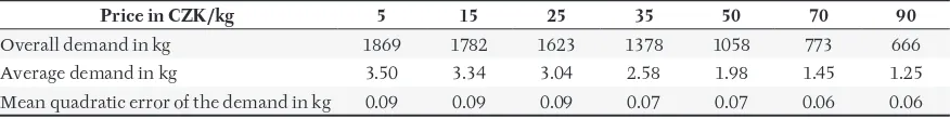
The following data concerning demand for bread have been obtained from the questionnaire research; they have been incorporated into the table as well as into the graph.
From the graph of demand it follows clearly that the demand for bread is the classic curve/course corresponding to the law of diminishing demand. The average demand ranges (within the scope of the price range) from 3.50–1.25 kg per month per one member of the household.
If we consider the price elasticity at the so called common price (round CZK 30), marked in the graph of the price elasticity by the green dashed lines, we obtain the value of 0.48 from the interval 0.36–0.6 determined by the mean quadratic error.
III: Table of values of the price elasticity of the j kind of goods (our own processing)
Price in CZK ( 1 2)
2
j j
P P ( 2 3)
2
j j
P P ( 3 4)
2
j j
P P ( 4 5)
2
j j
P P ( 5 6)
2
j j
P P ( 6 7)
2
j j
P P
Elasticity EDj1 EDj2 EDj3 EDj4 EDj5 EDj6
Standard deviation
of elasticity SEDj1 SEDj2 SEDj3 SEDj4 SEDj5 SEDj6
IV: Table of estimate of weights of the j kind of goods in the consumer basket at the given price (our own processing)
Price in CZK Pj1 Pj2 Pj3 Pj4 Pj5 Pj6 Pj7
Price index of the consumer
basket in % CPIj1 CPIj2 CPIj3 CPIj4 CPIj5 CPIj6 CPIj7
V: Table of values of the demand for bread (our own processing)
Price in CZK/kg 5 15 25 35 50 70 90
Overall demand in kg 1869 1782 1623 1378 1058 773 666
Average demand in kg 3.50 3.34 3.04 2.58 1.98 1.45 1.25
When compared with the value of the coeffi cient of price elasticity of demand for bread in the USA, amounting to 0.15 (Aguirre, 2010) and/or 0.108 (Gwartney, 2005), the demand for bread is to a certain degree less non-elastic in the Czech Republic, nevertheless estimate of the price elasticity for all kinds of baker’s ware is 0.22 in the Czech Republic (USDA, 2005), which is very close to the established value.
If we analyze development of estimated bread weight in the consumer basket at diff erent prices, it is evident that at the usual price the value amounts to 0.90 %, which is very close to the ČSÚ data: 0.68 % (ČSÚ, 2010) (Tab. VII).
Coca-Cola
Coca-Cola is certainly the commodity non-essential for the common man and therefore we can await that the demand could be rather elastic. It is true that Coca-Cola is the beverage of characteristic taste that became popular all over the world thus belonging to typical commodities of the global beverage market; on the other side there is a number of beverages trying to compete Coca-Cola by similar taste (Tab. VIII).
We can persuade ourselves that the average demand per one person drops from 2.76 litre up to 0.06 litre per month within the price range from 1
0 20 40 60 80 100
0,00 0,50 1,00 1,50 2,00 2,50 3,00 3,50
Q [kg] P [Kþ/kg]
1: Curve of average demand − bread (our own processing)
VI: Values of the price elasticity of demand for bread (our own processing)
Price in CZK 10 20 30 42,5 60 80
Elasticity 0.05 0.19 0.49 0.74 0.93 0.59
Mean quadratic error of elasticity 0.04 0.08 0.12 0.12 0.16 0.25
0,00 0,20 0,40 0,60 0,80 1,00 1,20
0 5 10 15 20 25 30 35 40 45 50 55 60 65 70 75 80 85 P [Kþ/kg] Elasticita
E
D2: Price elasticity of demand for bread (our own processing)
VII: Table of estimate of the bread weight(s) in the consumer basket at the given price (our own processing)
Price 5 15 25 35 50 70 90
Czech crown per one litre up to 62 Czech crowns per one litre (Tab. IX)
From the graph of price elasticity of demand for Coca-Cola two facts can be pinpointed. The fi rst fact concerns confi rmation of the assumption, because demand is in the given price fi eld predominantly elastic. Coca-Cola is really used rather as a festive so drink than a common beverage for thirst quenching. The demand reaches the unit elasticity at the price of 18 CZK/lt. Below this price it is the non-elastic commodity with the potential to replace
the beverages in the consumer basket purchased by the households much more cheaper. The common price is rather high among other beverages, in spite of it Coca-Cola does not face any sales problems. We can claim here that the Coca-Cola brand benefi ts from the global popularity of this beverage on the one side and on the other side a certain snobbish eff ect can play a certain role here, determining a clear diff erence between the consumer who purchases Coca-Cola for drinking and between the consumer who purchases a pure table water. VIII: Table of values of the average demand for Coca-Cola (our own processing)
Price in CZK/l 1 5 11 20 30 42 62
Overall demand in l 1476 862 490 304 152 70 34
Average demand in l 2.76 1.61 0.92 0.57 0.28 0.13 0.06
Mean quadratic error of demand in l 0.35 0.15 0.08 0.07 0.03 0.02 0.01
0 10 20 30 40 50 60 70
0,00 0,50 1,00 1,50 2,00 2,50 3,00 3,50
Q [l] P [Kþ/l]
3: Curve of the average demand – Coca-cola (our own processing)
IX: Value of price elasticity of the demand for Coca-Cola
Price in CZK/lt 3 8 15,5 25 36 52
Elasticity 0.39 0.73 0.81 1.67 2.22 1.80
Mean quadratic error of elasticity 0.11 0.16 0.26 0.39 0.48 0.50
0,00 0,50 1,00 1,50 2,00 2,50 3,00
0 10 20 30 40 50 60
Cena [Kþ/l Elasticita
E
DP [K
þ
/l]
Another very interesting fact is that the unit elasticity is reached at the price of 18 CZK/lt, which is just the common price. It has to be added here that prices of diff erent packs diff ering by their volume rise with the falling volume and therefore determination of the common price was based on the declared quantities purchased by the households monthly at the given price. These quantities are purchased by the customers in the multipacks (six bottles with two Coca-Cola litres in each), the common price of which corresponds to 18 CZK per litre. At this price the elasticity reaches 1.00 from the range 0.70–1.30. This fact evidences
a very good marketing approach of the Coca-Cola company selecting the price level so that its receipts may be maximized.
Determination of the weight in the consumer basket was carried out for this commodity, the preceding commodity alike. These weights at the given price can be found in the table below; the weight of 0.13% corresponds to the usual price, which is a little bit more than the offi cial ČSÚ data, i.e. 0.11% (ČSÚ, 2010), (Tab. X).
X: Table of estimate of the Coca − Cola weight in the consumer basket at the given price (our own processing)
Price in CZK/lt 1 5 11 20 30 42 62
Consumer basket in % 0.03 0.10 0.12 0.13 0.10 0.07 0.05
SUMMARY RESULTS
For better illustration the examined commodities will be arranged in the table by the rising price elasticity corresponding to the common price (Tab. XI).
XI: Commodities arranged by the price elasticity
Serial
number Commodity
Price elasticity at the common price
Common price in CZK/unit
Price in CZK/unit corresponding to the
unit elasticity
1 Salt 0.04 5 -
2 Cold water 0.10 70 1251
3 Toothbrush 0.20 30 -
4 Socks 0.24 25 -
5 Cigarettes 0.25 70 752
6 Petrol 0.38 30 42
7 Eggs 0.40 2,5 3,75
8 Bread 0.48 30 502
9 Winter footwear 0.50 1500 2600
10 Instant coff ee áva 0.62 0,7 0,9
11 Jeans 0.64 1000 19002
12 Dinner in the restaurant 0.70 120 150
13 Rice 0.78 40 46
14 Dra beer 0.80 50 68
15 Tomatoes 0.85 44 50
16 Private education 0.80−1.00 100−200 295
17 Cinema visiting 0.95 150 125
18 Coca-cola 1.00 18 18
19 Fish fi llet 1.25 110 98
20 Beef from the rump 2.95 170 90
The next table shows conformity or possible distinction/dissimilarity of values of the price elasticity of demand for the chosen commodity with the values established for the USA. The United States are applied, because adequate data volumes are available for diff erent periods and these values are commonly used for comparison (Gwartney, 2005), (Aguirre, 2010), (Baye, 2006).
XII: Commodities arranged by dissimilarity of the price elasticity in the Czech Republic and in the USA (our own processing)
Commodity
Price elasticity at the common price in the
Czech Republic
Price elasticity in the USA Distinction in elasticity
Tomatoes 0.85 4,60 yes
Coca-cola 1.00 3.8 yes
Beef from the rump 2.95 0.40–0.64 yes
Dinner in the restaurant2 0.70 2.3 yes
Fish fi llet 1.25 0.5 yes
Bread 0.48 0.108–0.15 yes
Eggs 0.40 0.1 yes
Instant coff ee 3 0.62 0.25–0.30 partially
Rice 0.78 0.55 partially
Winter footwear 3 0.50 0.7 partially
Cigarettes 0.25 0.4–0.48 partially
Petrol 0.38 0.2 partially
Private education 0.80–1.00 1.1 no
Dra beer 3 0.80 0.3–0.9 no
Toothbrush 0.20 0.1 no
Salt 0.04 0.1 no
Cinema visiting 0.95 0.9 no
Cold water 0.10 – –
Socks 0.24 – –
Jeans 0.64 – –
REFERENCES
AGUIRRE, C. M., 2011: Elasticity of Demand and Supply [online]. [cit. 2011-06-02]. Source: http://faculty. mdc.edu/caguirrl/Outline6.htm.
BAYE, M., 2006: Managerial Economics and Business Strategy. New York: McGraw − Hill, 620 p.
BECKER, G. S., 1997: Teorie preferencí. Praha: Grada Publishing, 352 p. ISBN 80-7169-463-0.
BLATNÁ, D., 2004: Metody statistické analýzy. Praha: BIVŠ, 92 s. ISBN 80-7265-062-9.
Český statistický úřad, 2010: Spotřební koš pro výpočet indexu spotřebitelských cen od ledna 2010 [online] [cit. 2010-06-02]. Source: http://www.czso.cz/ csu/redakce.nsf/i/spotrebni_kos_2010/$File/spot_ kos2010.xls.
SUMMARY
DEZANKOVÁ, H., 2007: Analýza dat z dotazníkových šetření. Praha: Professional Publishing, 212 p. ISBN 978-80-86946-49-8.
Economic Research Service. International Food Consumption Patterns, 2010: [online]. [cit. 2010-06-02]. Source: http://www.ers.usda.gov/data/ InternationalFoodDemand.
FRANK, R. H., 1995: Mikroekonomie a chování. Praha: Nakladatelství Svoboda, 765 p. ISBN 25-042-95. GWARTNEY, J. D. et al., 2005: Economics: Private and
Public Choice. South − Western/Cengage Learning. ISBN 9780324205640.
HINDLS, R. et al., 2007: Statistika pro ekonomy. 8. vyd. Praha: Professional Publishing, 415 p. ISBN 978-80-86946-43-6.
HUŠEK, R. PELIKÁN, J., 2003: Aplikovaná ekonometrie: teorie a praxe. Praha: Professional Publishing, 263 p. ISBN 80-86419-29-0.
KEŘKOVSKÝ, M., 2004: Ekonomie pro strategické řížení: teorie pro praxi. Praha: C.H. Beck, 184 p. ISBN 80-7179-885-1.
PECÁKOVÁ, I. NOVÁK, I., HERZMANN, J., 1998: Posuzování a vyhodnocování dat ve výzkumech veřejného mínění. Praha: VŠE v Praze, 146 p. ISBN 80-7079-357-0.
SCHILLER, B. R., 2004: Mikroekonomie dnes. Brno: Computer Press, 404 p. ISBN 80-251-0109-6.
Address