THE SINGULAR VECTOR APPROACH TO THE ANALYSIS OF PERTURBATION GROW TH IN THE ATMOSPHERE
by Roberto Buizza
March 1997
ProQuest Number: 10017276
All rights reserved
INFORMATION TO ALL USERS
The quality of this reproduction is dependent upon the quality of the copy submitted.
In the unlikely event that the author did not send a complete manuscript and there are missing pages, these will be noted. Also, if material had to be removed,
a note will indicate the deletion.
uest.
ProQuest 10017276
Published by ProQuest LLC(2016). Copyright of the Dissertation is held by the Author.
All rights reserved.
This work is protected against unauthorized copying under Title 17, United States Code. Microform Edition © ProQuest LLC.
ProQuest LLC
789 East Eisenhower Parkway P.O. Box 1346
A B STR A C T
This dissertation applies linear algebra to the study o f perturbation growth in atmospheriç flows. Maximally-growing perturbations are identified from singular vector analysis of the time-evolving flow.
Given a system characterized by a linear propagator L(tQ,t), which describes the time evolution of small perturbations x between time tg and t
around a time-evolving trajectory, an inner product on the tangent space of the perturbations defined by a matrix E and its associated norm ||..||g, the problem can be stated as:
♦ Find the phase space directions x fo r which is maximum, where x(t)=L(tg,t)x(to).
Given the adjoint L*^ of the forward propagator L , perturbation growth is gauged by computing the eigenvectors o f an operator including L and L*^
as factors. The eigenvectors with the largest eigenvalues define the directions with maximum growth. They are called the singular vectors of the tangent forward propagator L.
First, the singular vector approach is described.
Second, a barotropic model of the atmospheric flow is considered. The impact o f underlying orography on singular vectors growing over different time intervals, and the role of singular vectors in explaining the maintenance of blocked flows during winter, are analyzed.
Third, a 3-dimensional primitive equation model of the atmospheric flow is considered. Some aspects of the application o f the singular vector technique to the study of perturbation growth in the whole atmosphere are analyzed. A physical interpretation of singular vector growth based on the application o f the Eliassen-Palm theorem and on WKBJ theory is proposed.
TABLE OF CONTENTS
1 Introduction 11
1.1 Stability in hydrodynamic flows 11
1.2 Stability in mathematics 14
1.3 Perturbation growth in the atmosphere 15
1.4 The normal mode approach to instability analysis 18
1.5 Perturbations growing during finite-time intervals:
the singular vector approach 20
2 Mathematical formalism 23
2.1 Singular vector definition 23
2.2 Projection operators 27
2.3 Pseudo-inverse and sensitivity fields 29
2.4 Singular vectors, normal modes and adjoint modes 31
2.5 The Lanczos algorithm 33
3 The impact o f orographic forcing on barotropic unstable
singular vectors 39
3.1 Introduction 40
3.2 The barotropic model 44
3.3 The adjoint technique 46
3.4 Singular vectors of idealized basic states 49
3.4.1 Singular vectors o f Rossby-Haurwitz waves 50
3.4.2 Singular vector sensitivity to orographic forcing
projecting onto a single spectral component 54
3.5 Singular vector sensitivity to simple orographies 64
3.5.1 Impact of simple orographies on singular vectors of a basic state super-position of a super-rotation and a RH-wave 61 3.6 Impact o f a real orography on singular vectors o f realistic
basic states 67
3.6.2 Impact of a realistic orography on the singular
vectors of a mean winter state 71
3.7 Conclusions 79
4 On the role o f finite-time barotropic instability during
transition to blocking 83
4.1 Introduction » 84
4.2 Methodology 88
4.2.1 The barotropic model 88
4.2.2 Linearization and definition of finite-time
unstable perturbations 89
4.2.3 Projection of tendency fields onto singular vectors 90
4.3 Atmospheric circulation during winter 1990/91 93
4.4 Properties and representativeness o f barotropic singular vectors 98 4.4.1 Intra-seasonal variability o f a barotropic instability index 98 4.4.2 Location o f the fastest growing singular vectors 102 4.4.3 Projections of tendency fields onto singular vectors 104
4.5 Case studies 108
4.5.1 10-14 December 1990 (day 10-14) 110
4.5.2 22-26 and 26-30 December 1990 (days 22-26 and 26-30) 110
4.5.3 12-16 January 1991 (day 43-47) 112
4.5.4 21-25 and 25-29 January 1991 (day 52-56 and 56-60) 112
4.5.5 22-26 February 1991 (day 84-88) 114
4.6 Experiments with time-invariant basic states 117
4.7 Discussions and conclusions 121
5 Aspects o f a 3-D singular vector computation for the
atmosphere 131
5.1 Impact of Non-linear Normal Mode Initialization 133
5.2 Impact o f surface drag and vertical diffusion 134
5.3 Impact of horizontal diffusion 138
5.4.1 Impact of horizontal resolution 142
5.4.2 Impact of vertical resolution 148
5.5 Impact of the initial time inner product 149
5.6 Impact of the optimisation time interval on singular vectors 157
6 A physical interpretation o f singular vector growth 159
6.1 The Eliassen-Palm theorem in the quasi-geostrophic
approximation on the beta-plane 159
6.2 W ave propagation under W KJB theory 165
6.3 Characteristics of T21L19 singular vectors 169
7 Two operational applications o f the singular vector
technique 193
7.1 The ECMW F Ensemble Prediction System 193
7.2 Targeting observations using singular vectors 203
8 Conclusions 207
Acknowledgements 211
Chapter 1
INTRODUCTION
This work focuses on the analysis of the growth of small perturbations in atmospheric flows during finite-time intervals. Considering a system described by a set o f non-linear differential equations^ a methodology, based on the solution of an eigenvalue problem of the tangent forward and adjoint propagators of the system equations, is used to identify perturbations that can amplify during finite-time intervals. Although this work does not study whether systems can sustain growing instabilities as usually defined in literature (Sections 1.1 and 1.2), it can be considered as a stability analysis with attention focused to phenomena occurring on a finite time range.
The rationale for studying the problem of perturbation growth during finite time intervals is made clear by the discussion o f the problem of numerical weather prediction (Section 1.3). The singular vector approach is different from the normal mode method which is usually applied in literature in dynamic stability analyses (Section 1.4), and shows that non-normal structures can grow over finite time intervals also in neutral or stable situations (Section 1.5).
1.1 Stability in hydrodynamic flows
Helmholtz, Kelvin, Rayleigh and Reynolds recognized the importance of hydrodynamic stability already in the nineteen century. As noted by Drazin and Reid (1981), stability problems are very clearly introduced by Reynolds'
(1883) description of a series of experiments on the instability of flow in a pipe:
The ... experiments were made in three tubes ... The diameters of these were nearly
1 inch, 1/2 inch and 1/4 inch. They were all ... fitted with trumpet mouthpieces, so that the
water might enter without disturbance. The water was drawn through the tubes out of a large
glass tank, in which the tubes were immersed, arrangements being made so that a streak or
The general results were as follows;
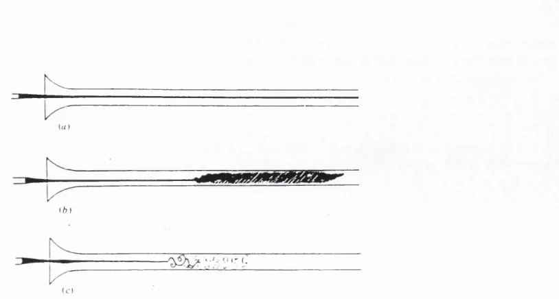
(1) When the velocities were sufficiently low, the streak of colour extended in a
beautiful straight line through the tube. Fig. 1.1a.
(2) If the water in the tank had not quite settled to rest, at sufficiently low velocities,
the streak would shift about the tube, but there was no appearance o f sinuosity.
(3) As the velocity was increased by small stages, at some point in the tube, always
at considerable distance from the trumpet or intake, the colour band would all at once mix up
with the surrounding water, and fill the rest o f the tube with a mass of coloured water, as*in
Fig. 1.1b. Any increase in the velocity caused the point of break down to approach the
trumpet, but with no velocities that were tried did it reached it. On viewing the tube by light
o f an electric spark, the mass o f coloured resolved itself into a mass o f more or less distinct
curls, showing eddies, as in Fig. 1.1c.
Reynolds showed that the laminar flow described in paragraph (1) breaks down when the Reynolds number R e= V a/v exceeds a certain critical value, V being the maximum velocity of the water in the tube, a the radius of the tube, and v the kinematic viscosity of water at the appropriate temperature. Reynolds estimated that in his experimental set up, the critical value Re^ was ~ 13,000. However,
... the critical velocity was very sensitive to disturbances in the water before entering the tubes
... This at once suggested the idea that the condition might be one o f instability for disturbance
o f a certain magnitude and stable for smaller disturbances.
At critical velocity
... another phenomenon ... was the intermittent character of the disturbance. The disturbance
would suddenly come on through a certain length of tube and pass away and then come on
again, giving the appearance of flashes, and these flashes would often commence successively
at one point in the pipe. The appearance when the flashes succeeded each other rapidly was
as shown ...
in Fig. 1.2. Such flashes are now called 'turbulent spots'.
ib)
(•' (.
F ig u r e 1.1. (a): l a m i n a r f lo w in a p ip e; (b): t r a n s it io n to tu r b u le n t flo w in a p i p e ; (c): t r a n s i t i o n to t u r b u l e n t fl o w as s e e n w h e n i l l u m i n a t e d b y a s p a r k . ( F r o m R e y n o l d s .
1883.)
stability. Following Drazin and Reid (1981), the transition from laminar flow to turbulence can be explained qualitatively as follows. Below the critical Reynolds number there is a laminar Poiseuille flow with a parabolic velocity profile, stable to infinitesimal disturbances. Some way below the observed critical Reynolds number a finite disturbance may grow if it is not too small. Above the critical Reynolds number, quite small disturbances grow rapidly with a sinuous motion. Soon they grow so much that non-linearity becomes strong and large eddies (Fig. 1.1c) or turbulent spots (Fig. 1.2) start to appear.
The importance o f the study o f the stability analysis of solutions of equation o f motions is clearly stressed by Landau and Lifshitz (1951):
... In solving the equations of steady flow for a viscous fluid, it is often necessary to
make certain approximations on account of mathematical difficulties. The validity o f these
approximate solutions is, of course, restricted ...
In principle, however, there must be an exact stationary solution o f the equations of
fluid dynamics for any given steady external conditions ...
Yet, not every solution of the equation of motion, even if it is exact, can actually
occur in Nature. The flows that occur in Nature must not only obey to the equations o f fluid
dynamics, but also be stable. For the flow to be stable it is necessary that small perturbations,
if they arise, should decrease with time. If, on the contrary, the small perturbations which
inevitably occur in the flow tend to increase with time, than the flow is absolutely unstable ...
1.2 Stability in mathematics
Consider an N dimensional system, and suppose that the hnear differential equations describing the motion of small perturbations u' around a solution u
have constant coefficients (this approximation is made only to simplify the formalism, but can be generalized to systems described by differential equations with non-constant coefficients). The N-th order linear differential equations can be written as
Following Birkhojf and Rota (1969), the homogeneous linear equation (1.1) is strictly stable when every solution tends to zero as /—><»; it is stable when every solution remains bounded as r—>0 0; when not stable, it is called
unstable.
The homogeneous linear equation (1.1) is strictly stable if and only if it has a finite basis of solutions tending to zero, and stable if and only if it has a basis of bounded solutions [where a basis erf solutions is a set of n solutions such that the general solution of (1.1) can be expressed as a linear combination o f them].
If the coefficients of Eq. (1.1) are real, it can be proved that Eq. (1.1)
has a basis of solutions of the form t: t ^ e ^ ^ s in v t , t ^ e ^^co sv t ,
with r, ti, V real constants. Thus, a solution of this kind tends to zero if and only if }i<0, and it remains bounded as > 0 0 if and only if ji<0 or pi=r=0.
(These results can be proved more generally for linear differential equations with constant complex coefficients.)
1.3 Perturbation growth in the atmosphere
The atmosphere constitutes an example of an intricate dynamical system with many degrees o f freedom. The state o f the atmosphere consists o f the spatial distribution of wind, temperature, and other weather variables (e.g. specific humidity and surface pressure). The mathematical differential equations describing the system time evolution are an expression of the physical laws that describe the behaviour of the atmosphere. One of them is Newton's laws of motion used in the form "acceleration equals force divided by mass"
{Lorenz, 1993), others include the laws of thermodynamics which describe the behaviour of temperature and the other weather variables. Thus, generally speaking, there is a set of differential equations which describe the weather evolution, at least in an approximate form.
with a set of algebraic difference equations for the tendencies of various field variables at a finite number o f grid points in space. By extrapolating the computed tendencies ahead in time, he could predict the field variables in the future. Unfortunately, his results were very poor, both because of deficient initial data, and because o f serious problems in his approach.
After World W ar II interest in numerical weather prediction revived, partly because o f an expansion o f the meteorological observation network, but also because of the development of digital computers.
Charney (1948) developed a model applying an essential filtering approximation of the Richardson's equations, based on the so-called geostrophic and hydrostatic equations. In 1950, an electronic computer (ENIAC) was installed at Princeton University, and Charney, Fjortoft and Von Neumann and Ritchmeyer (1950) made the first numerical prediction using the equivalent barotropic version of his model. This model provided forecasts of the geopotential height near 500 hPa, and could be used as an aid to provide explicit predictions o f other variables as surface pressure and temperature distributions.
Chamey's results led to the developments o f more complex models of the atmospheric circulations, the so-called global circulation models. An example of such models is the operational model implemented at the European Centre for Medium-Range Weather Forecasts (ECMWF). Its current formulation {Courtier et al., 1991; Simmons et a i , 1995) is based on a horizontal spectral triangular truncation T213, it is characterized by 31 vertical levels, and it includes a parametrization of many physical processes such as surface and boundary layer processes {Viterbo and Beljaars, 1995) radiation
{Mocrette, 1990), and moist processes {Tiedtke, 1993; Jacob, 1994).
Generally speaking, the current status and limitations of numerical weather prediction can be summarized as follows.
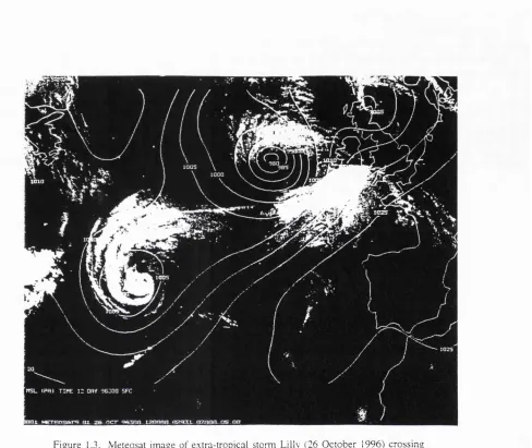
F ig ure 1.3. Meteo sat im age o f extra-tro pical storm Lilly (26 O c to b e r 1996) crossin g the Atlantic, s u p e r im p o s e d to su rface pre ssu re ( mb).
with many data.
The limitations to weather forecasting are related to the incomplete description of all physical processes (model uncertainties or errors), and to the presence of uncertainties in the initial state due to the limited number of data available (initial conditions' uncertainties or errors). It should be stressed that, since each data is characterized by an error which depend on the instrumental accuracy, there will always be errors in the initial conditions. In other words, small uncertainties related to the characteristics o f the atmospheric observing system will always characterize the initial conditions.
This was first pointed out in meteorology by Lorenz (1965), who noted that even if the system equations were well known, two initial states differing only slightly from each other could diverge very rapidly as time progresses. Subsequently, Somerville (1979) showed that observational errors, usually in the smaller scales, amplify and through non-linear interactions spread to longer scales, eventually affecting the whole flow field.
As shown by simple hydro-dynamical system (Section 1.1), small uncertainties introduced in a system can amplify and induce a drastic change of the system flow. In the case o f numerical weather prediction, errors in the initial conditions could amplify and quickly deteriorate a weather forecast. This makes very difficult the prediction o f severe storms, like the one which crossed Britain during the night between the 28th and the 29th o f October 1996 (Fig. 1.3).
1.4 The normal mode approach to instability analysis
The method more commonly applied to study the stability o f particular solutions o f a dynamical system is based on normal modes, whereby small disturbances are resolved into modes, which may be treated separately because each satisfies the linear system which describes the time evolution of the small disturbances themselves.
dx
— =X{x) , (1-2)
at
and let a be a critical point (i.e. a point where all the functions X, are equal to zero).
■ DEFINITION L I . The critical point a is called
(i) stable when, given e>0, there exists a ô>0 so small that, if
|x (0 )-a |< 0 , then \x (t)-a \< e fo r all t>0;
(ii) asymptotically stable when, fo r some 0>0,
|x (0 )-a |< 0 implies lim^ ^ |x ( 0 - a | =0 ;
(Hi) strictly stable when it is stable and asymptotically stable.
A stable critical point which is not asymptotically stable is called neutrally stable; a critical point which is not stable is called unstable.
In particular, suppose that X (x)= A x in Eq. (1.2), i.e. consider the constant-
coefficient linear autonomous system x(t) = A x . Define as a norm al m ode
a solution of the form %(r) =e^^f . The following theorem on the stability of
the critical point 0 for this system can be proved.
■ THEOREM 1.1. The critical point 0 o f the constant-coefficient linear
autonomous system x {i)= A x is asymptotically stable i f and only if
every eigenvalue o f A has negative real part. In this case, the system is also strictly stable.
0 can be reduced to an eigenvalue problem, specifically to the analysis of the existence of eigenvectors of A with positive real part.
Focusing on atmospheric flows, by considering an idealized basic state with vertical shear only and by applying a normal mode stability analysis,
Chamey (1947) and Eady (1949) isolated the baroclinie instability mechanism, and showed that the zonal mean component o f realistic mid-latitude tropospheric flow is unstable. The resulting exponentially growing structure proved to have length and time scales similar to observed atmospheric cyclogenesis. Normal modes were also used, for example, by Simmons et al.
(1983) to examine the barotropic instability o f a zonally varying time-mean state, and to show that their time behaviour was consistent with the most rapidly growing normal mode.
1.5 Perturbations growing during finite-time intervals: the singular vector approach
Farrell (1982) studied the growth o f perturbations in baroclinie flows. He noted that the long time asymptotic behaviour is dominated by discrete exponentially growing normal modes. However, other physically realistic perturbations are possible, that amplify over a given finite time interval more than the most unstable normal mode.
... Perturbations to stationary solutions of the equations for baroclinie flows are able
to extract energy from the mean state, whether exponentially growing instabilities are allowed
or not. In cases with such exponential modes, the degree to which the mode is excited is
dependent on the initial condition so that the initial set up o f the instability may proceed much
more rapidly than would be predicted for the pure normal mode initial condition. ...
The adjoint of a dynamical model was first used for sensitivity studies by Kontarev (1980) and Hall and Cacuci (1983). Later on, Le Dimet and Talagrand (1986) proposed an algorithm, based on an appropriate use of an adjoint dynamical equation, for solving constraint minimisation problems in the context of analysis and assimilation of meteorological observations. More recently, Lacarra and Talagrand (1988) applied the adjoint technique to determine optimal perturbations using a simple numerical model. Following
Urban (1985) they used a Lanczos algorithm {Strang, 1986) in order to solve the related eigenvalue problem. For a bibliography in chronological order of published works in meteorology dealing with adjoints up to the end of 1992, the reader is referred to Courtier et al. (1993).
Chapter 2
MATHEMATICAL FORMALISM
The theoretical and numerical aspects o f the computation of perturbations characterized by the fastest growth over a finite time interval are discussed in this chapter.
Given a set of non-linear differential equations describing the dynamics of a generic system, first the tangent equations are deduced and the tangent propagator is constructed, then an inner product is defined in the tangent space, and finally the adjoint propagator is defined (Sections 2.1). Projection operators used in the studies reported in Chapters 3-5 to address specific questions are also introduced (Section 2.2). The mathematical formalism and the definitions come essentially from linear algebra. The treatment is general, and can be applied to any system described by a set o f differential equations.
As mentioned in Chapter 1, the computation o f the fastest growing perturbations can be reduced to an eigenvalue problem. Due to the very large number of degrees of freedom that can characterize systems such as the atmosphere, the eigenvalue problem can be solved only by algorithms that do not need to access directly the matrix elements that define the problem. A Lanczos algorithm has been implemented for this purpose (Section 2.3).
2.1 Singular vector definition
Let X be the state vector of a generic autonomous system, whose evolution equations can be formally written as
0Y
- f =A(X) .
(2.1)
ot
Denote by x (0 an integration o f Eq. (2.1) from îq to t which generates a trajectory from an initial point Xo to
model equations
dx
where A^= 6A(x)/6x\^^^^ is the tangent operator computed at the trajectory
point x(0
-Let L(t,to) be the integral forward propagator o f the dynamical equations (2.2) linearized about a non-linear evolving trajectory x ( 0
x(t)=L(t,t^) x(t^) ,
(2.3)
that maps a perturbation x at initial time Iq to its value at the optimisation time
t. (Since L is a linear operator, it can be represented by a matrix, and we will use the same symbol for the operator and the matrix.) The tangent forward operator L maps the tangent space % the linear vector space o f perturbations at to IIj, the linear vector space at X r
Consider two perturbations jc and y, e.g. at Xo^ ^ positive definite Hermitian matrix E , and define the inner product )g as
(x;y)^ = <x'JEy>
(2.4)
on the tangent space I Iq. Here is the canonical Euclidean scalar product,
=
.
(2.5)
Let ||..|1e be the norm associated with the inner product )g,
\\xf
=
(x;x)
=
<x;Ex>
.
(2.6)
= . (2.7)
The adjoint of L with respect to the inner product defined by E can be written in terms o f the adjoint V defined with respect to the canonical Euclidean scalar product as
. (2.8)
From Eqs. (2.3) and (2.7), it follows that the squared norm of a perturbation x at time t is given by
l|jc(f)l^= W f„);i’^ i x ( y ) ^ . (2.9)
Let us now recall the problem we want to address (see Abstract):
♦ Find the phase space directions x fo r which lx(t)\^ / ||jr(fo)||g is maximum, where x(t)=L{to,t)x(ÎQ).
Equation (2.9) shows that this problem can be reduced to the search of the eigenvectors
L * ^ £ v /ï^ ) = a^v,(i^) , (2.10)
with largest eigenvalues a f.
The square roots of the eigenvalues, a,, are called the singular values
and the eigenvectors the (right) singular vectors of L with respect to the inner product E (see, e.g.. Noble and Daniel, 1977). The singular vectors with largest singular values identify the directions characterized by maximum growth. The time interval î-èq is called optimisation time interval.
dimensional tangent space of the perturbations at Xo' Moreover, the eigenvalues are real, a^>0.
At optimisation time r, the singular vectors evolve to
, (2.11)
which in turn satisfy the eigenvector equation
= . (2.12)
From Eqs. (2.9) and (2.12) it follows that
l|vX01^ = of .
(2.13)
Since any perturbation %(f)/||%(f^)||^ can be written as a linear combination
of the singular vectors v/r), it follows that
\\x m ^
Thus, maximum growth as measured by the norm ||..||e is associated with the dominant singular vector v^.
Given the tangent forward propagator L, it is evident from Eq. (2.10) that singular vectors' characteristics depend strongly on the inner product definition and on the choice of the optimisation time interval (e.g., this means that the eigenvalues a / depend on the optimisation time interval).
IWOIL
< L x ( t \ ^ L x ( t >
(2.15)
0
is maximum. Applying the coordinate transformation the right hand side of Eq. (2.15) can be transformed into
<LE^^%(t^y,ELE^^'^yiÇ>
(2.16)
Since
£ ' ’' * i * £ L £ ‘’“ = ( £ ' ‘'* L B "” ^)* (E ~^'^LE~^'^ , (2.17)
0 0 ^ 0 0
the phase space directions which maximize the ratio in Eq. (2.16) are the singular vectors of the operator with respect to the canonical Euclidean inner product. With this definition, the dependence o f the singular vectors' characteristics on the inner products is made explicit.
2.2 Projection operators
and the ECM W F primitive equation model) solve the system evolution equations partly in spectral space, and partly in grid point space.
Denote by Xg the grid point representation of the state vector jc, by 5 the spectral-to-grid-point transformation operator, Xg^Sx, and by GXg the multiplication of the vector Xg, defined in grid point space, by the function
g(s):
g(s) = l l / S 6 S
"
g ( î ) = O i / î î S ’
where s defines the coordinate of a grid point, and 27 is a geographical region. Define the function w(n) in spectral space as
w(n) = l i f n e Q
w(n) =0 i f n c Q ’ t • ;
where n identify a wave number and D is a sub-space of the spectral space, and by W x the multiplication of the state vector x by the function w(n).
Consider a vector x. The application of the local projection operator r , defined as T ^ ’^GS, to the vector x sets the vector x to have zero grid point values outside the geographical region 27. Similarly, the application of the spectral projection operator W to the vector x sets to zero its spectral components with wave number outside Û.
The projection operators T and W can be used at either the initial or the final time, or at both times. Their usefulness is evident, for example, from the formulation of the following problem: find perturbations with (i) fastest growth during the time interval (ii) unit Eg norm and wave components belonging to Qq initially, and (Hi) at the optimisation time, maximum E norm measured inside the geographical region 27 and with wave components belonging to Qj.
Such a problem can be solved by the computation of the singular vectors of the operator
K ^ E '^ '^ T S L S E '^ '^ . (2.20)
2.3 Pseudo-inverse and sensitivity field
Following Buizza et al. (1997), consider the set of the first M singular vectors of the N dimensional space of a system with M<.N (for example, N -4 8 4 for a T21 barotropic model, and N ~ l& for a T21L19 primitive equation model of the atmosphere, and M~10-10^). During the optimisation time interval, this set of singular vectors define what we call the unstable sub-space o f the system. It is convenient to introduce a normalized set of evolved singular vectors ii,- with unit norm, so that
v.(0
u = — . (2.21)
* o
Denote by V=[Vj(îq), .., ViJtg)] the NxM matrix with columns v / y , by U-[Uj, u^] the N xM matrix with columns and by 27 the M xM diagonal matrix with elements cr,. Then, applying Eq. (2.11), Eq. (2.21) can be written as
U '^ = L V . (2.22)
Equation (2.22) can be used to estimate the tangent forward propagator L in the unstable sub-space,
L ^ U H V " . (2.23)
Consider an arbitrary [for example, x(t) can be the difference between two solutions Xi and X2 of the non-linear model equations (2.1)]. The projection o f x(t) onto the unstable sub-space spanned by the evolved singular vectors v /0 can be written as
. (2.24)
Suppose that the initial state is unknown. From Eq. (2.23), it follows that an estimate o f the inverse of the tangent forward propagator is given by
and an estimate o f the initial state x(tg) is given by
x ( Ç = L *(r) = V S ■* tA ’x(t) . (2.26)
Equation (2,26) is the analogue, in the unstable sub-space, of inverting the forward propagator L to obtain the initial state. With respect to the full N
dimensional space, L is the Moore-Penrose pseudo-inverse {Penrose,
1955; Golub and Van Loan, 1983) of L, in the approximation where all the singular values outside the unstable sub-space are small compared with those inside the unstable sub-space. So, in this approximation,
. (2.27)
Consider now the problem o f finding a vector s(to )^s(t) that has the largest projection onto x(t), or in other words that maximizes the inner product
(s{t);x{t))^ . (2.28)
Since s(t)=Ls(to), and applying the adjoint definition, the inner product (2.28) is maximized when
s ( f ^ ) ~ £ * \( f ) . (2.29)
The vector s(to) is often referred to as a sensitivity field (following, for example, Marchuk, 1974, Cacuci, 1981). Since x(t)=Lx(to), it follows from Eq. (2.29) that
s ( t ^ ~ L '^ L x { Ç . (2.30)
Note that Eq. (2.10) can be written in matrix form as
and thus Eq. (2.30) can be written as
. (2.32)
In the hypothesis that the initial vector x(to) is unknown and applying Eq. (2.26), the sensitivity field can be estimated by
s ( t ^ ~ V Z , u ’x{t) . ' (2.33)
The comparison of Eqs. (2.26) and (2.33) shows that the estimated initial state x {t^
and the estimated sensitivity field differ only in the weighting of the
singular vectors used in the projection.
2.4 Singular vectors, normal modes and adjoint modes (The following Section has been extracted from Buizza and Palmer, 1995.)
The notion of singular vector analysis can be considered as a generalization of the classical normal mode instability analysis. This can be made explicit by linearizing the set of non-linear differential equations (2.1) about a stationary solution, so that the linear operator does not depend on time.
Normalized eigenvectors ^ of Ay with eigenvalues pi^
A Ç. = 1A.£. , (2.34)
give rise to normal mode solutions of Eq. (2.2),
n = l e ^ . (2.35)
j j
The integral operator can be written as
L ( t , t ) = e , (2.36)
with eigenvectors ^ and eigenvalues e
In general, the linear operators associated with realistic stationary basic state flows are non-normal because of vertical and horizontal wind shear
{Farrell and Moore,
1992).
Because of this, the normal modes are not orthogonal to one another. However, irrespective of normality, n o rm ali^ d eigenvectors rjj and eigenvalues dj of the adjoint operator L*^ must, from Eq.(2.7),
satisfy the bi-orthogonality condition( U -0 “ )(T1,;O =0 ,
(2.37)
J J J J ^
where is the complex conjugate of dj. This condition ensures that the eigenvalues of an eigenvector/adjoint eigenvector pair that are not orthogonal m ust form a complex conjugate pair. The magnitude o f the inner product
( depends on the angle Yj the two eigenvectors subtend in phase space.
Zhang
(1988)
defines1
_
(2.38)
COSY
J J J ^
the projectibility of (j.
Let us suppose that the normal modes have a finite eigenvalue spectrum, and that they constitute a basis. Then, any vector x can be written as
. (2.39)
From Eq. (2.39), the fastest growing normal mode will ultimately dominate the linear combination. Hence, for sufficiently long optimisation times, the dominant singular vector at optimisation time will correspond to the most unstable normal mode.
In order to maximize the contribution from the first normal mode at optimisation time, Cj in Eq. (2.39) should be as large as possible. If % (y=^y, then C;=7. By contrast, if x(tQ)=r\j, then Cj is maximized {Zhang, 1988), with
Ci=llcosYj in the hypothesis of the normal and adjoint modes being normalized to have unit norm at initial time. Hence, at initial time, the dominant singular vector will be determined by the first adjoint eigenvector, whilst at (indefinitely long) optimisation time the dominant singular vector is determined by the first normal mode itself.
This is illustrated schematically in Fig. 2.1 for an idealized 2- dimensional system with decaying normal modes. The singular value will depend on both the e-folding time of the dominant normal mode and its projectibility.
For finite optimisation times, the dominant singular vectors will no longer project onto individual normal modes and their adjoints, and the amplification rate o f the singular vectors will not be bounded by properties o f the dominant normal modes alone.
2.5 The Lanczos algorithm
A
--Figure 2.1. T h is diagram illustrates schem atically the crucial difference betw een normal m ode and singular vector growth, and the relationship between singular vectors and adjoint m odes. A n idealized 2-D system has tw o very non-orthogonal d ecaying modes and W e take to have larger real eigenvalue com ponent. The adjoint m odes tJj and TJ2 are show n, with tJj, orthogonal to ^ and f / , resp ectively (according to the bi-orthogonahty condition (2.37)). A normalized vector is show n parallel to 7 7 Its tim e evolution can be estim ated by mapping the tip and tail o f Vg
along the and ^ directions (show n as dashed lines) using the m odal decay rates. The sequence o f vectors v„, n = l , 2, .. givin g the time evolution o f Vg increases in amplitude up to so m e finite n-=N, and is aligned alm ost entirely with for large n.
Consider the eigenvalue problem
A x = a , x , (2.41)
where A=ICK, and K is the operator defined in Eq. (2.20). By definition, the matrix A is NxN dimensional, and symmetric. Without loss o f generality, we can also suppose that it is real. ^
If A is a real, symmetric matrix, then there exists an orthogonal real matrix Q such that
q 'A Q = D (X ^ ,..,X ^ , (2.42)
where D(Àj, À2) is a diagonal matrix, and denotes the transpose o f Q (Schur decomposition theorem).
The Lanczos algorithm does not directly compute the diagonal matrix D, but it first computes a partial transformation of the matrix A using a tridiagonal matrix T
q 'a q =t , (2.43)
with
a
P
0 .
h “ 2 P3 °
0 P3
T= ■ 0
0
P .-. 0
° Py-I “ y-i P ;
. 0 P , a .
and with
0 = ■ (2.45)
where the vectors qj are column vectors, and where the number of iterations
J is much smaller than the dimensionality o f the problem, J ^ N . Then, the Lanczos algorithm finds the diagonal decomposition of T
T ^s 'dS . (2.46)
The elements o f the diagonal matrix D are an estimate o f the eigenvalues of A, and an estimate of the eigenvectors are given by Y=[yj, y J , with
Y = Q S . (2.47)
The actual computation is performed by writing Eq. (2.43) as
A Q = Q T . (2.48)
Equating columns of Eq. (2.48), it follows that
for j= l, J. The orthogonality of the vectors qj implies that
OL_=q*Aq, . (2.50)
Moreover, if
r = ( A - a . i )3 .-P ^ j (2.51)
is non-zero, then
r
where P ~ ± y/<rj;rp>. An iterative application o f these equations, with a randomly chosen starting vector defines the Lanczos iterative procedure. The total number of iterations J determines the accuracy o f the computation. As this number increases, more eigenvalues/eigenvectors can be separated from the others, independently of the choice of starting vector q^. This separation starts from the extremes of the eigenvalue spectrum. The accuracy o f the eigenvectors is less than the accuracy o f the singular values, say to order e
when the precision of the singular values is o f order é .
Chapter 3
THE IMPACT OF OROGRAPHIC FORCING ON BAROTROPIC UNSTABLE SINGULAR VECTORS
(The following Chapter is the text o f Buizza, 1995b.)
The influence of topography on fluid instability has been studied in literature both in the beta channel approximation and on the sphere mainly using normal modes. A different approach recently proposed is based on the identification of unstable singular vectors, i.e. structures that have the fastest growth over finite time intervals. Systems characterized by neutral or damped normal modes have been shown to have singular vectors growing (e.g. in terms of kinetic energy) over finite time intervals. Singular vectors do not conserve their shape during time evolution as normal modes do. Various aspects related to the identification o f singular vectors of a barotropic flow are analyzed in this paper with the final goal of studying the impact of the orography on these structures.
First, we focus on very idealized situations to verify if neutral and damped flows can sustain structures growing over finite time intervals. Then, we study singular vectors o f basic states defined as the super-position o f a super-rotation and a Rossby-Haurwitz wave forced by orographies that project onto one spectral component only, or forced by very simple orographies with longitudinally or latitudinally elongated shapes. This first part shows that orography can alter the unstable sub-space generated by the most unstable singular vectors, either directly through the action of the orographic term in the linear equation or indirectly by modifying the evolution of the basic state.
In the second part we consider a realistic basic state, defined as a mean winter flow computed from three months of observed vorticity field, forced by a realistic orography. We show that the orographic forcing can indirectly modify the singular vector structures. In fact "orographically induced" instabilities can be identified only when considering time-evolving basic states.
can be captured by the adjoint technique.
3.1 Introduction
The impact o f topographic forcing on the flow of a barotropic atmosphere has been widely recognized and studied in literature. Charney and DeVore (1979) showed that the occurrence of multiple stationary or oscillatory equilibrium states can be related to external forcing. They analyzed th e impact of topographic and thermal forcing on equilibrium solutions of a highly truncated spectral model o f the barotropic atmosphere, and were able to show how topographic forcing relates to equilibrium solution structures. One o f the conclusions o f their work was that topographic instability might be responsible for transitions between different meta-stable states.
Following Charney and DeVore (1979), Frederiksen and Bell (1987) showed that topography plays an important role in the formation of some large-scale teleconnection patterns. In later works, Frederiksen (1989) and
Frederiksen and Bell (1990) examined the role of barotropic and topographic instability during periods o f persistent blocking, and indicated that topographic instability plays little role in the mechanism o f block formation.
The influence of underlying topography on the instability of a fluid has been studied both in the beta-channel approximation and on the sphere.
Fyfe and Derome (1986), studying the stability of free and forced planetary waves in a beta-channel with a barotropic model, analyzed the interaction of unstable (normal mode type) perturbations with the bottom orography. They demonstrated that a forced zonal wave can be stable or unstable depending on the amplitude of the topography, and they concluded by reporting the existence of travelling topographically unstable waves.
examined the instability properties of the fluid using a linearized version of a barotropic vorticity equation following the normal mode approach.
Hoskins (1973) studied the stability of Rossby-Haurwitz waves (hereafter RH waves) for a single planetary wave and a zonal flow in spherical geometry. Supported by some numerical integrations, he concluded that RH
waves with zonal wave m ^ 5 are stable whilst those with m>5 may be
unstable. However, his numerical procedure permitted only zonal wave numbers that are multiples of 4, so other types of disturbances were prohibited.
Baines (1976) analyzed the stability of planetary waves to small disturbances as an eigenvalue problem deduced from the linearisation of the non-divergent barotropic vorticity equation, in spherical geometry and without topographic forcing. He showed that waves with total wave number n less than 3 are stable, whereas those with total wave number greater than 3 are unstable if the amplitude of the perturbation is large enough.
The consensus of these authors was that the barotropic approximation is sufficiently accurate to describe the basic mechanisms o f topographic forcing, resonance and nonlinear interactions. In a work by Legras and Ghil
(1985), it is suggested that a simple barotropic model is capable of simulating the actual behaviour of the large-scale mid-latitude atmospheric flow, whose spatial structure is known to be barotropic to a large extent (Blackmon et a i,
1979). Baroclinie instabilities occur on scales smaller than the barotropic instabilities, and their characteristic time scales are shorter than those considered.
A different approach to the instability analysis has been used by Farrell
(1982, 1988), who pointed out that normal modes are not the fastest growing perturbations over finite time intervals. By superimposing two Orr (1907) solutions with different initial tilts of the phase lines in the horizontal plane,
perturbation can be expressed in terms o f the truncated operator's normal modes; however, they are not in general orthogonal. As a consequence, linear combinations o f two or more modes can grow much faster than any individual mode. Unlike normal modes, these structures change over time since their growth is space dependent. They are called unstable singular vectors, and they are defined as the directions in the phase space of the system that give the largest growth o f the norm of a state vector x (see section 3.2 for more details)
over the optimisation time interval They can be computed using the tangent and the adjoint versions of the non-linear model describing the system evolution (Lacarra and Talagrand, 1988).
In a later work Boyd (1983), studying analytically a linear Couette flow, confirmed the results of Farrell (1982) and concluded that to understand the mechanism o f finite time interval growth one should consider not only the discrete normal modes but also the continuous spectrum of singular neutral modes. [As shown by Pedlosky (1964) they form a complete set for the canonical Eady (1949) and Charney (1947) problems.] On a later work, studying small error dynamics, Farrell (1990) proved that the increase of the errors on synoptic time scales is controlled by stmctures that are not o f normal mode form.
Borges and Hartmann (1992) studied the barotropic stability of observed 300 hPa non-zonal flows searching for singular vectors. They demonstrated that they are at least as important, for stability considerations, as the adjoint and eigenmode stmctures.
(at initial time) by unstable singular vectors have much larger growth rates than normal modes and possess a more localized spatial structure. Comparing the singular vectors computed using the two models, they showed that the baroclinie singular vectors are more localized in the meridional direction, with little amplitude in the tropics and with a maximum closer to the jet core than the barotropic singular vectors. They found barotropic singular vectors with amplification rates similar to the baroclinie vahies for optimisation times shorter than 2 days. However, for longer optimisation time intervals baroclinie singular vectors are characterized by larger amplification rates, since they grow as a result of both baroclinie and barotropic energy conversions. Considering smooth time-invariant basic states defined to identify two regimes of the northern hemisphere winter flow, they showed that barotropic singular vectors evolve in closer agreement to forecast errors than the baroclinie singular vectors. Finally, they concluded that barotropic singular vectors appear to be able to generate regime transitions.
Barotropic models and the adjoint technique have been used also in variational assimilation studies. Talagrand and Courtier (1987) and Courtier and Talagrand (1987) showed how the adjoint equation o f a non-divergent barotropic vorticity model can be used in the problem of assimilation of meteorological observations.
The adjoint technique is applied throughout this study. A non-linear spectral barotropic model in spherical geometry, its tangent and adjoint versions have been coded. The model has been written so that the time integration of the tangent and the adjoint versions are performed following the trajectory described by the basic state.
This work concentrates on singular vector rather than on normal mode type instabilities. Our purpose is to study the impact of the topography on the singular vectors. Table 3.1 is a schematic of the work presented in the paper.
growing over finite time intervals. Then, in sub-section 3.4.2, we analyze the impact of simple orographies projecting onto one spectral component only on the singular vectors of idealised basic states, defined as the superposition of a super-rotation and a RH wave. In section 3.5 we consider more localized but still idealized orographies, and we study their impact on the singular vectors of the same basic states considered in sub-section 3.4.2. Finally, in section 3.6, we study whether "orographically induced" perturbations csa be identified when considering a realistic basic state forced by a realistic topographic forcing. Conclusions are drawn in section 3.7.
Section Basic-state flow Orography Study
3.4.1 (n,m) RH wave --- normal modes vs sing. vect.
3.4.2 Srot + (n,m) RH wave (n,m) forcing orographic impact on sing. vect. 3.5.1 Srot 4- (n,m) RH wave idealized orographic impact on sing. vect. 3.6.2 Obs atmospheric flow real orographic impact on sing. vect.
Table 3.1. Schematic o f the subjects analyzed in each Section.
3.2 The barotropic model
The numerical model used for this study has been derived from the vorticity equation in spherical geometry
■ ^ = / ( f + / ( i + - ^ ) ; « - — C - — a'c , (3.2)
diffusion processes have been set respectively to 10 day and to 10 day/m^.
The model is solved in the coordinate system defined by the longitude
À and the sine of the latitude ii=sin(j). A non-dimensional equation has been deduced from Eq. (3.2), with the space coordinates scaled by the earth radius
a and the time scaled by twice the earth angular velocity Ü
X ^ _
X —— , t — 'ZÇit , (3.3)
a
where jc, t are the dimensional variables. The non-dimensional equation has
been discretized through a truncated expansion o f spherical harmonics, at triangular truncation T21, and the equation for the time evolution o f the vorticity expansion coefficients has been numerically integrated using a time filtered Leapfrog scheme.
The linearized equation for a perturbation C follows from Eq. (3.2) by
writing the vorticity as the sum of a mean value C and a perturbation C
■ ^ = 7 ( f ; i i ; ) + 7 ( C + / ( l + - ^ ) ; > |> ) - 2 - f — J _ a'C . (3.4)
K &
The adjoint o f Eq. (3.4) with respect to the canonical Euclidean norm
IlCf s <C;C> = /■ f ' r f S , (3.5)
J z
can be analytically computed from Eq. (3.4)
^ = y ( i : ; i P ) + A ' ‘y ( C + / ( i + - ^ ) ; C ) + 3 - c + _ L A ' c . (3.6)
K " w
K E = - j J iliCrfS . (3.7)
Using Eq. (3.4) in Eq. (3.7), we can derive an equation for the perturbation kinetic energy evolution
■ ^ = r + f i | r ) r f S . (3.8)
ot
J'L
Jn
h
0
The first term on the right hand side represents the advection o f the perturbation kinetic energy by the basic state flow. The second term gives the exchange of energy between the perturbation and the basic state, the third term describes the orographic forcing and the fourth term represents all the dissipative processes of the model.
If we consider Eqs. (3.2) and (3.4) without any dissipation mechanism, both the stream function o f the mean state and o f the perturbation satisfy the following equation
where the left hand side of Eq. (3.9) is the area average of the angular momentum. Thus, in the absence o f orography (and of dissipations) this quantity is conserved.
3«3 The adjoint technique
Let % be a state vector in the phase space o f the system. The evolution equation (3.2) can be formally written as
^ ■ A W ,
(3.10)
The most unstable singular vectors are the directions in the phase space of the system that guarantee the fastest growth of the norm of the perturbations over a finite time interval. For small time intervals and small initial amplitudes their behaviour is almost linear, and they can be computed using the linearized equation
d x
— = A x , ^ (3.11)
where A = — 1_ is the tangent operator that corresponds to the model
I dx
operator A.
Let us denote the propagator of Eq. (3.11) by L=L(t,to). The perturbation x(t) at time t is then given by
x{t) = L x { t ^ ) . (3.12)
Let us define an inner product on the space of the perturbations
{r,y) = <x\Ey> , (3:13)
where E defines some weighting factors, and is the canonical Euclidean scalar product. Let us define the associated norm of a generic vector
\ \ x f = (x;x) = <x ; Ex > , (3.14)
with the weights E defined so that the norm (3.14) of a perturbation is its kinetic energy. The norm of the perturbation at time t is given by
U U ) t = {L x-,L x) . (3.15)
(L ^x;y) = ( x; Ly) . (3.16)
Then, using the definition (3.16) in (3.15), the norm of the state vector x(t) at time t can be computed as
||* (f)f =
( i
x^-,L x^)
= (L
‘L x^,x^\ .
(3.17)
The square roots o f the eigenvalues o f o f the matrix L*^L are called the singular values o f the matrix L, and the eigenvectors v, of the matrix L*^L are called the right singular vectors o f L.
The singular vectors v, identify an orthogonal base in the phase space of the system (Buizza et al., 1993). They are orthogonal at time tg and at final time t . The singular values a, give the amplification factors between t g and t
for each of them, and they are functions of the optimization time interval t - t g .
As demonstrated by Farrell (1989) and Borges and Hartmann (1992), the singular vectors with the largest singular values identify the perturbations growing fastest over the optimisation time interval.
The method we implemented to solve this eigenvalue problem is based on a Lanczos algorithm (see Strang, 1986) developed by the Numerical Algorithm Group (NAG, Oxford).
To compare singular vector structures we can define the N-dim unstable sub-space relative to an experiment as the sub-space o f the phase space of the system defined by the first N singular vectors. We can compare unstable sub spaces generated by the first N singular vectors Vj of two experiments A and B using a projection matrix M(A,B;N) whose elements are
m ..(A ^ ) = <vfA);E v,(B)>^ . (3.18)
of the A experiment which is explained by the j-th singular vector of the B experiment. The sum of the matrix elements with a fixed first index represents how well the i-th singular vector o f the A experiment can be reconstructed from a linear combination of the first N singular vectors of the B experiment.
We can also define a "similarity index" of two experiments A and B, that measures the similarity of the unstable sub-spaces generated by the first
N singular vectors of each experiment
s(AyB;N) - — m_{AJS) . (3.19)
Some reference values for the similarity index, obtained with the barotropic model, are reported hereafter:
a) singular vectors that identify the same unstable sub-space are characterized by s(A,B;N)=100%\
b) orthogonal unstable sub-spaces are characterized by s(A,B;N)=0;
c) the mean similarity index, averaged over winter '90-'91, computed between unstable sub-spaces of two consecutive days generated with a
48h optimisation time interval, is s(day;day+1;20) = 45% ;
d) the mean similarity index, averaged as in c), but computed between unstable sub-spaces generated by the singular vectors o f day d and of
day d+2, is s(day;day+2;20) = 30% .
3.4 Singular vectors o f idealized basic states
of the flow is analyzed in sub-section 3.4.2, where we consider orographic forcing that projects on the (n,m) spectral component only, and flows superposition o f a super-rotation and a (n,m) RH wave.
We concentrate on RH waves with total and zonal wave numbers equal to (2,1), (4,1) and (8,1). The choice m = l has been made so that in a latitudinal belt there is a region o f convergence (representing a jet stream) and a region o f divergence. Other zonal wave numbers are not considered since we are more interested in changing the meridional than the zonal vorticity gradients. Starting from total wave num ber «=2, we study waves with increasing total wave number n=4 and n=8 to have more small scale features in the basic state characteristics.
3.4.1 Singular vectors o f Rossby-Haurwitz waves Baines (1976) deduced from the results of Fjortoft (1953) an inequality concerning the spectral distribution o f energy for a barotropic model without any dissipation term and with no orography in spherical geometry. He found that if the initial energy is in a mode or modes with total wave number n>2,
then the RH wave can be unstable if the wave amplitude is sufficiently large. Thus, the (2,1) RH wave has stable normal modes, while the (4,1) and the (8,1) RH waves can have unstable normal modes. For each wave, we analyzed the sensitivity of the unstable normal modes to the initial wave amplitude
if = if P + c.c.
m /i m,n
= 2R g(if )P cos(wiA)- 27/n(if )P sin(mA) . (3.20)
m,n m,n m,n
Let US define the e-folding time o f a normal mode b y
1
T ^ , (3.21)
where o>^ is the real part of the normal mode frequency.
Figure 3.1 shows the e-folding time of the most unstable normal mode as a function of the non-dimensional vorticity amplitude. The (4,1) and the (8,1) RH waves are unstable if the wave amplitude is larger than a given threshold, while the (2,1) RH wave is stable independently of the basic state amplitude.
Singular vectors of the (2,1)^, (4,1) and (8,1) RH waves have been computed for different optimisation time intervals keeping the basic state constant. A time-independent basic state was chosen because for unstable or damped systems the fastest growing singular vector computed with constant basic state approaches the most unstable normal mode in the limit /-^oo. Let us define the amplification factor X{t) and the parameter v{t) for a singular vector by
« . ) . J g ! .
(3.22,
" '> ■ t o ® » ■
where the norm has been computed using Eq. (3.14). r(rj gives the time required for the perturbation norm to increase by a factor e, precisely the definition of the e-folding time of a normal mode. Thus z{t) will be referred to as the e-folding time o f the singular vector.
The basic state amplitude of the three RH waves, in terms of the non- dimensional vorticity field, has been fixed to the same value
Re(C ) = 0, 7m(C )=0.1 . (3.24)
m,n
1000
100-1
— ' 1 0
-Ui 2 I -o
£
LÜ0.1
-0.0 1
-0.001
1000
V0R/(2 OMEGA)
Figure 3.1. Ordinate: e-folding times 7=11 (day) o f the m ost unstable normal m ode o f the (4,1) RH w aves (dashed line) and o f the (8,1) RH w ave (dotted line). Abscissa: non-dimensional vorticity amplitude o f the RH w ave. A reference line corresponding to an e-folding tim e o f 1-day has been drawn. (From Buizza, 1995b.)
UJ p 10-o
£
lii
o n (DAYS)
a) >-< Q lli 2 P Q Ui 20 15 10 5 0 16 10 12
6 8 14
0 2 4
on
(DAYS)
Figures 3.2a and 3.2b show, respectively, the e-folding times of the fastest growing singular vector of the (2,1) and (8,1) RH waves (solid lines). [Since, for each optimisation time interval, the e-folding times of the singular vectors of the (4,1) RH waves are very similar to the (8,1) ones, they are not shown.] The singular vectors of all the three RH waves are slowly growing, with e-folding times longer than 7 days. We can see that the singular vectors relative to the (2,1) RH wave are unstable, and that for the (8,1) RH wave the e-folding time of the 1st singular vector computed with any o f the considered optimisation time interval is lUO of the minimum normal mode e-folding time. Figure 3.2 shows that the e-folding time increases with the optimisation time interval. All these optimisation time intervals are too short for the fastest growing singular vector to approach the e-folding time o f most unstable normal mode. [The increase of the singular vector e-folding time with the optimisation time interval is also partly due to a small horizontal diffusion term included in the numerical model to avoid numerical instabilities (see Eq. (3.2)) which decreases the singular vector energy.]