Scholarship at UWindsor
Scholarship at UWindsor
Electronic Theses and Dissertations Theses, Dissertations, and Major Papers
2009
Discovering the size of a deep web data source by coverage
Discovering the size of a deep web data source by coverage
Jie Liang
University of Windsor
Follow this and additional works at: https://scholar.uwindsor.ca/etd
Recommended Citation Recommended Citation
Liang, Jie, "Discovering the size of a deep web data source by coverage" (2009). Electronic Theses and Dissertations. 326.
https://scholar.uwindsor.ca/etd/326
This online database contains the full-text of PhD dissertations and Masters’ theses of University of Windsor students from 1954 forward. These documents are made available for personal study and research purposes only, in accordance with the Canadian Copyright Act and the Creative Commons license—CC BY-NC-ND (Attribution, Non-Commercial, No Derivative Works). Under this license, works must always be attributed to the copyright holder (original author), cannot be used for any commercial purposes, and may not be altered. Any other use would require the permission of the copyright holder. Students may inquire about withdrawing their dissertation and/or thesis from this database. For additional inquiries, please contact the repository administrator via email
by
Jie Liang
A Thesis
Submitted to the Faculty of Graduate Studies through the School of Computer Science in Partial Fulfillment of the Requirements for
the Degree of Master of Science at the University of Windsor
Windsor, Ontario, Canada 2009
c
by
Jie Liang
APPROVED BY:
Dr. Huapeng Wu
Department of Electrical and Computer Engineering
Dr. Luis Rueda School of Computer Science
Dr. Jianguo Lu, Advisor School of Computer Science
Dr. Jessica Chen, Chair of Defense School of Computer Science
Author’s Declaration of Originality
I hereby certify that I am the sole author of this thesis and that no part of this thesis has been published or submitted for publication.
I certify that, to the best of my knowledge, my thesis does not infringe upon anyone’s copyright nor violate any proprietary rights and that any ideas, techniques, quotations, or any other material from the work of other people included in my thesis, published or oth-erwise, are fully acknowledged in accordance with the standard referencing practices. Fur-thermore, to the extent that I have included copyrighted material that surpasses the bounds of fair dealing within the meaning of the Canada Copyright Act, I certify that I have ob-tained a written permission from the copyright owner(s) to include such material(s) in my thesis and have included copies of such copyright clearances to my appendix.
Abstract
.
Acknowledgements
My thanks and appreciation to Dr. Jianguo Lu for persevering with me as my advisor throughout the time it took me to complete this research and write the thesis, and for his guidance on my research and during the course of my graduate study which are the most important experiences in my life.
I am grateful as well to Dr. Richard A. Frost for his instructions on conducting a litera-ture review and survey on the topic of my thesis. Especially, I need to express my gratitude and deep appreciation to Dr. Jessica Chen who encouraged and enlightened me on the way of critical thinking in the early stages of my graduate study and research.
Author’s Declaration of Originality iii
Abstract iv
Dedication v
Acknowledgements vi
List of Figures ix
List of Tables xi
1 Introduction 1
2 Related Work 5
2.1 TheCapture Histories with Regressionmethod . . . 6
2.2 Broder et al.’s method . . . 7
2.3 The OR Method . . . 7
3 The Experiment System and Data Collections 9 3.1 The system . . . 9
3.1.1 Overview . . . 10
3.1.2 Data Flow . . . 11
3.2 The data collections . . . 12
3.2.1 Characteristics of data collections . . . 12
3.2.2 Indexing the data collections . . . 15
3.3 Evaluation metrics . . . 16
4 The Pool-based Coverage Method 18 4.1 A naive estimator . . . 18
4.2 The large variance and high cost problem . . . 23
4.3 Constructing a query pool . . . 27
4.3.1 Learning the query pool from another existing corpus (C2) . . . 28
4.3.2 Learning the query pool from a sample ofD(C3) . . . 30
4.4 Summary . . . 39
5 The Comparison 43 5.1 The experiment of the CH-Reg Method . . . 43
5.2 The experiments of Broder’s method . . . 45
5.2.1 ConstructingQPB by terms fromD . . . 45
5.2.2 ConstructingQPB by terms from a sample ofD . . . 47
5.2.3 Summary . . . 47
5.3 The experiment of the OR Method . . . 49
5.4 The experiments on Chinese corpora . . . 52
5.5 The comparative study . . . 55
5.5.1 Methods that need to download documents . . . 55
5.5.2 Methods that only need to check IDs . . . 59
5.5.3 The overall comparison . . . 62
6 Conclusions 66
Bibliography 69
A Glossary of Notations 76
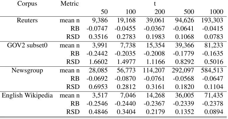
3.1 The System Overview . . . 10 3.2 The Service Data Flow . . . 11 3.3 The document size distribution of all corpora. . . 14
4.1 Scatter plot of 100 estimations method C1. For GOV2 subset0, 100 words are randomly selected from the 40,000 Webster words, RSD=1.0415. For English Wikipedia, 1000 words are randomly selected from the 40,000 Webster words, RSD=0.2205. . . 25 4.2 Scatter plot of query weight overdf on the four corpora. . . 26 4.3 A comparison between C1 and C2. The data are from Table 4.3 and Table
4.6. . . 31 4.4 A comparison between C2 and C31. The data are from Table 4.6 and Table
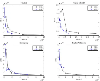
4.8. . . 34 4.5 A comparison between C31 and C32. The data are from Table 4.8 and Table
4.10. . . 38 4.6 Weight of terms from a sample ofDand weight of random words
distribu-tion over df. . . 39 4.7 Weight of terms from a sample ofDand weight of random words
distribu-tion over df. (Switched) . . . 40
5.1 A comparison of Broder’ method - B1 and B0. Data are collected from Table 5.4 and Table 5.5. . . 48 5.2 A comparison of C32 and Broder’s Method practical version (B0) on large
English Corpora by MSE-Cost plots. Data are obtained from Table 5.5 and Table 4.10. . . 56 5.3 A comparison of C32 and Broder’s Method practical version (B0) on large
English Corpora by RB-Cost plots. Data are obtained from Table 5.5 and Table 4.10. . . 57 5.4 A comparison of C32 and Broder’s Method practical version (B0) on large
English Corpora by RSD-Cost plots. Data are obtained from Table 5.5 and Table 4.10. . . 58
5.5 The OR Method, CH-Reg Method and C32 on 100,000 documents English Corpora. Data are obtained from Table 5.1, Table 5.6 and Table 4.11. . . 59 5.6 The OR Method, CH-Reg Method and C32 on 500,000 documents English
Corpora. Data are obtained from Table 5.1, Table 5.6 and Table 4.11. . . 60 5.7 The OR Method, C32 and CH-Reg Method on Chinese Corpora. Data are
obtained from Table 5.8, Table 5.9 and Table 5.10. . . 61 5.8 The OR Method, C32, CH-Reg Method and B0 on English Corpora. Data
are obtained from Table 5.1, Table 5.5, Table 5.7 and Table 4.10. . . 62 5.9 The OR Method, C32, CH-Reg Method and B1 on English Corpora. Data
are obtained from Table 5.1, Table 5.4, Table 5.7 and Table 4.10. . . 63 5.10 The OR Method, C32, CH-Reg Method and B0 on English Corpora. Data
3.1 The corpora summary. Cells marked by ‘-’ mean data are not available. . . 13 3.2 TheFields in each LuceneDocumentobject. . . 15
4.1 The matrix represents a set of queries with the documents that they can capture. Cells marked by ‘1’ mean a document match a query. . . 19 4.2 The statistical data of the query pool of C1. . . 23 4.3 The estimation by C1 on four English corpora. Data are obtained by 100
trials, each trial is produced by randomly selectingtnumber of queries from
QP. . . 24 4.4 The notations of Pool-based Coverage Method. The sample size is 3000 for
C3X. . . 28 4.5 The statistical data of the query pool for C2. The query pool has 40,340
queries. . . 29 4.6 The estimation by C2 on five English corpora. Data are obtained by 100
trials, each trial is produced by randomly selecting t number of queries fromQP. . . 30 4.7 The statistical data of the query pool of C31. . . 33 4.8 The estimation by C31 on four English corpora. Data are obtained by 100
trials, each trial is produced by randomly selectingtnumber of queries from
QP. . . 33 4.9 The statistical data of the query pool of C32. . . 36 4.10 The estimation by C32 on five large English corpora. Data are obtained by
100 trials, each trial is produced by randomly selectingtnumber of queries fromQP. . . 36 4.11 The estimation by C32 on small English corpora. Data are obtained by
100 trials, each trial is produced by randomly selectingtnumber of queries fromQP. . . 37 4.12 Coverage of queries when query document frequencies are smaller then a
certain value. Queries are from Webster dictionary. It shows that rarer words can not cover all the data source. . . 41 4.13 The statistical data of query pools of C1, C2, C31 and C32. . . 42
5.1 A summary of the CH-Reg Method experiment on English corpora. Cells marked by ‘-’ mean data are not available. Each trial randomly selects 5,000 queries the Webster Dictionary and discards any query that returns less than 20 documents. In each query, only top 10 matched documents are returned. . . 44 5.2 Broder’s method notations . . . 45 5.3 The coverage of medium frequency terms of its corpus . . . 46 5.4 Estimation using Broder’s method - B1. RB and RSD are calculated by 100
trials. . . 46 5.5 Estimation using Broder’s method - B0. RB and RSD are calculated by 100
trials. . . 49 5.6 Estimating small English corpora using the OR Method. Bias and
stan-dard deviation of the estimation over 100 trials. In each trial, queries are randomly selected from 40,000 Webster words. . . 50 5.7 Estimating large English corpora using the OR Method. Bias and standard
deviation of the estimation over 100 trials. In each trial, queries are ran-domly selected from 40,000 Webster words. . . 51 5.8 A summary of the CH-Reg Method experimental data on Chinese corpora.
Cells marked by ‘-’ mean data are not available. Each trial randomly se-lects 5,000 queries from the Contemporary Chinese Dictionary and discards any query that returns less than 20 documents. In each query, only top 10 matched documents are returned. Bias and standard deviation of the esti-mation over 100 trials. . . 53 5.9 Estimating Chinese corpora using the OR Method. Bias and standard
devi-ation of the estimdevi-ation over 100 trials. In each trial, queries are randomly selected from Contemporary Chinese Dictionary. . . 53 5.10 The estimation by C32 on Chinese corpora. Data are obtained by 100 trials,
each trial is produced by randomly selectingtnumber of queries fromQP. . 54 5.11 The size and coverage ofQPfor each corpora in Table 5.10. . . 54
Introduction
The deep web [8], in contrast to the surface web that can be assessed by following
hy-perlinks inside web pages, consists of the resources that can only be obtained via query
interfaces such as HTML forms [7] and web services [36]. Data from deep web are usually
generated from background databases of websites.
The size of a data source is a vital parameter used in the collection selection algorithms
in distributed information retrieval systems [41] [42] [40]. Also, estimating the size of a
data source is a necessary step of a deep web data crawler and data extractor [27] [7] [35]
[13] [14] [41] [32] [34] [39] [44] [20]. They need to know the size to decide when to stop
crawling. In addition, the size is an important metric to evaluate the performance of the
crawler and the extractor. Although the data source owner knows its size, that information
may not be available to the third parties.
The objective of the thesis is to estimate the number of documents a deep web data
source contains by sending queries. The estimation process starts with selecting queries.
Queries can consist of characters, words, phrases, or their combinations. The queries can be
randomly selected, or chosen according to their features such as their document frequencies.
After queries are issued to capture the documents in a data source, matched documents or
their IDs are returned. Using this data, several methods are developed to estimate the size.
In general, there are two approaches to estimating a data source size. One does not need
to download and analyze the documents. Instead, it only needs the document IDs. This
approach originates from a traditional Capture-Recapture model [38] [2] [15] [25] [17].
It analyzes the relation between the number of distinct documents and duplicates in the
captures [40] [29] [30] [9] [19] [43] [5] [45] [23] [24] [21] [11]. The basic estimator has
an underlying assumption: each object has equal probability to be captured. However, the
capture of documents cannot be random as they can only be retrieved by queries. The other
basic approach requires the downloading of the documents matched by queries [12] [6]
[33] [28]. It involves document content analysis, trying to find the relations between the
downloaded documents and the collection.
This thesis proposes a new coverage-based method for estimating the size of a data
source. This method constructs a query pool from which queries are selected. This query
pool should have high coverage of the collection but relatively low and similar document
frequencies. Once the query pool is built, we will randomly select and issue a number of
queries, download the documents that are captured, and compute the weight of the queries
[12] to estimate the size of the collection. If query pool is not carefully constructed, this
method will have negative bias, large variance, or a high cost. When the query pool cannot
cover all the documents, there will be a negative bias. When the query pool contains words
of very different document frequencies, there will be a large variance. When the query pool
has some popular words, the cost of estimation is high. Hence, we propose two ways to
construct a better query pool that can reduce the bias, variance, the number of queries, and
source. From this sample, we select queries that have similar document frequencies, and a
high coverage of the data collection. The other approach assumes a collection is available
to allow arbitrarily access. We utilize it, selecting a number of terms as the query pool that
covers more than 99% of this collection. Then, we use this query pool to estimate other
data source size.
This thesis conducts an extensive comparison between the new method and three
exist-ing estimation methods proposed by Shokouhi et al. [40], Broder et al. [12] and Lu [30],
respectively. We carry out experiments to produces the data of each method under our open
and flexible estimation framework. In the experiments, we collected four English and three
Chinese data collections to simulate actual deep web data sources. The performance of each
method is evaluated by bias, variance and cost. We issue different numbers of queries to
examine the cost and bias of a method. Furthermore, we issue the same number of queries
for 100 times to collect 100 estimates in order to measure the variance. In particular, we
investigate the impact of sample size on the estimation accuracy. All experimental data are
tabulated in tables and visualized in plots. Finally, a comprehensive comparison summary
demonstrates the capabilities of each method.
This thesis is organized as follows: before proposing the new method, we summarize the
related work. Researchers built different environments to evaluate their proposed methods.
These environments are not open to the public. Hence, it is difficult for others to carry out
experiments to compare existing methods with new ones. We create an open and flexible
estimation framework to provide estimation data via web services. This framework and
data collection we collected to evaluate methods are illustrated in Chapter 3. Chapter 4
describes our new approach based on Broder et al.’s concepts. In Chapter 5, we describe
comparison study of the four methods mentioned above. Finally, this thesis summarizes the
Related Work
There are two approaches to estimating a collection size. The first approach only needs to
examine the document identifiers. It originates from a traditionalCapture-Recapturemodel.
Methods based on this approach include theCapture Histories with RegressionMethod[40]
and the OR Method[29][30]. These methods analyze the relations between stepwise
over-lapping of documents, historically distinct documents and totally checked documents.
Be-cause the capture of documents is not precisely random as they can only be retrieved by
queries, they need to compensate for the bias introduced sampling document by queries.
The second approach needs to download and analyze document. It requires the
construc-tion of query pools and the downloading of the documents response to queries. Broder
et al. developed a method to measure how much a query from a pre-selectedQuery Pool
contributes to capturing the documents that the Query Pool can capture in total.
Further-more, they proposed a new estimation method by employing two query pools and applying
Peterson estimator [4].
2.1
The
Capture Histories with Regression
method
Shokouhi et al. [40] adapted the Capture-Recapture [38] technique used in ecology to
estimate corpus size. They proposed a correction to theCapture Histories (CH) method
and theMulti Capture Recapturemethod to compensate for bias inherent in sampling via
query-based sampling. The authors compensated for the bias using training sets and applied
regression analysis. The new methods are called the Capture Histories with Regression
(CH-Reg) andMulti Capture Recapture with Regression.
TheCH method issuestnumber of queries. Afteriqueries, it will count the number of
documents returned (ki), the number of documents in the returned documents that have all
been captured (di), and the total number of distinct documents that have ever been captured
(ui). The size of the collection (N) is estimated as [40]:
ˆ
N=∑
t
i=1kiu2i
∑ti=1diui
(2.1)
TheCH-Regcompensates for the bias by:
log(NCHˆ−Reg) =0.6429×log(N) +1.4208 (2.2) There are three constraints when collecting query returns in their experiments. One is
that only the top 10 documents are collected in each step. By default, a search engine has its
sorting method of query returns. In this case, we use the default sorting method of Lucene.
The second constraint is that any query that returns less than 20 documents is eliminated.
The third constraint is that CH-Reg sends 5,000 queries to obtain an estimated size of a
2.2
Broder et al.’s method
Broder et al. [12] proposed the following method (Broder’s method hereafter) to estimate
the size of a data collection: They firstly choose two query pools. For each query pool, by
issuing a random number of queries and calculating the weights of documents that can be
captured by a query, and the weights of queries, it can estimate the number of documents
that this query pool can capture. They estimate the overlap of two groups of documents
that captured by the two query pools by using one query pool and removing the documents
that contains no query in the other query pool. They estimateN by the traditional Peterson
estimator [4] ˆN=n1n2/nd (wheren1andn2are the sizes of two sets of document andnd is
the size of the intersection).
2.3
The OR Method
Lu [29][30] introduced a new term called the overlapping rate (OR) which is the
frac-tion of the number of accumulative documents returned by each query to the number of
unqiue documents obtained after i queries (Equation 2.4). The author approximated the
relation betweenORand the proportion of the corpus thatkicovered by a regression
analy-sis. Using the Newsgroup and Reuters data collections for training, the author obtained the
overlapping law in English corpora:
P=1−OR−1.1 (2.3) where
OR= ui
∑i1ki
And further derived the estimator:
ˆ
N= ui
The Experiment System and Data
Collections
3.1
The system
Building and accessing text corpora is a necessary step in the research when estimating the
size of deep web data sources. Because the size of corpora under investigation is too large
to be stored in one machine, multiple machines are involved in the experiments. We
pro-pose a new open and flexible framework to share the corpora via web service so that various
estimators can be experimented with. In this framework, it is easy to add new data
collec-tions, and they can be stored in different machines. The provided programmable interface
would allow third parties to query existing collections. Researchers, including people in
other research groups, can use their own program to configure query parameters and
is-sue queries. The framework is able to return stepwise estimation data likeki in Equation
2.1, and statistical data such as the query weight distribution. With the help of the proposed
framework, researchers will be able to evaluate the estimation performance and result of the
proposed method. It is also convenient to compare the estimation results of new methods
with existing methods.
3.1.1
Overview
The framework consists of three basic components depicted in Figure 3.1.
Figure 3.1: The System Overview
The estimation core is the program which accepts search arguments and queries, and
returns query results and statistical data. Each invocation of the core results in a query
process on one selected index. It has the predefined ability to access different type of
indexes. The output remains in the same format.
Service, which have many applications [1][26]. When the request is sent to one of the web
services, it will decompose the request to extract such information as the target collection,
the step size, sorting approach, and terms, and invokes the estimation core with extract
arguments and terms. When the core finishes a search, it will return the result to the web
service. The services then send the result back to the requester. These web services could
also provide the information of available collections.
The system is flexible in a way that the service could be invoked by other applications or
services which wants to make further use of the data. Also, the system could be duplicated
and each computer (node) could be in different machines. By a web service portal, the
nodes could work together to contribute to a more powerful system.
3.1.2
Data Flow
Figure 3.2: The Service Data Flow
The clients of web services send search parameters such as the name of the collection,
the step size, sorting approach and queries to the web service. The web services decompose
the request, and collect the profile of the desired collection; for example, the total number of
with decomposed requests as arguments to query on the selected index. The core records
the document IDs return by querying each term. If requested, it can provide various data for
exampleui,di, the document frequency (d f), the weight of each document, and the weight
of each query [12]. These data are returned to web services. The web services format the
query results and statistical data in XML format, and return them to clients. Note that in
order to reduce network traffic, it will only return requested data.
3.2
The data collections
In our experiment, we collected seven data collections which are popular in natural
lan-guage processing, information retrieval, and machine learning systems. They are TREC
GOV2 Collection [16], Reuters Corpus [37], Newsgroup Corpus, English Wikipedia
(enwiki-20080103-dump) and Chinese Wikipedia (zhwiki-20090116-dump) [18], a collection of
Chinese literature and Sogou Web Corpus [22]. The GOV2 and Sogou Web Corpus have
more than 10 million documents. In order to evaluate the methods for estimating
differ-ent sizes of corpora, we created a few random subsets theses corpora. All documdiffer-ents are
converted to UTF-8 encoding before indexing.
3.2.1
Characteristics of data collections
We collect various statistical data to provide the information of collection characteristics.
Table 3.1 is a summary of the data collections. Figure 3.3 shows the size distribution of
each collection. It shows that there are a few documents that have very large sizes and
Table 3.1: The corpora summary. Cells marked by ‘-’ mean data are not available. Corpus N Mean of SD of Mean of the SD of the
document document number of number size(Byte) size unique of unique
terms terms Reuters 806,791 1,553 1,264 125 82 Reuters 100k 100,000 1,612 1,331 125 83 Reuters 500k 500,000 1,617 1,329 125 82 Newsgroup 1,372,911 4,582 6,177 294 223 Newsgroup 100k 100,000 4,600 6,270 295 225 Newsgroup 500k 500,000 4,575 6,180 294 222 English Wikipedia 1,475,022 4,498 6,441 284 285 English Wikipedia 100k 100,000 4,513 6,472 285 289 English Wikipedia 500k 500,000 4,482 6,438 284 286 GOV2 subset0 1,077,019 10,842 22,796 396 409 GOV2 100k 100,000 10,934 22,871 395 401 GOV2 500k 500,000 10,811 22,783 396 407 GOV2 2M 2,000,000 10,919 22,747 396 410 Chinese Wikipedia 212,042 2,771 2,721 -
-2.5 3 3.5 4 4.5 0 1 2 3 4 5 6 7 8 log10(size) log10(occurence)
y = − 3.4*x + 16
Reuters linear
3 3.5 4 4.5 5 5.5
0 1 2 3 4 5 6 7 8 log10(size) log10(occurence)
y = − 2.2*x + 14
GOV2 linear
2.5 3 3.5 4 4.5 5
0 1 2 3 4 5 6 7 8
log 10 (size)
log 10 (occurence)
y = − 2.6*x + 14
Newsgroup linear
3 3.5 4 4.5 5 5.5
−1 0 1 2 3 4 5 6 7 log10(size) log10(occurence)
y = − 2.9*x + 16
English Wikipedia linear
2.5 3 3.5 4 4.5 5
0 1 2 3 4 5 6 log10(size) log10(occurece)
y = − 1.9*x + 10
Chinese Literature linear
1.5 2 2.5 3 3.5 4 4.5 0 1 2 3 4 5 6 7 log(size) log(occurence)
y = − 2*x + 9.5
Chinese Wikipedia linear
2.5 3 3.5 4 4.5 5 5.5 −2 0 2 4 6 8 10 log10(size) log10(occurence)
y = − 2.7*x + 15
Sogou linear
Table 3.2: TheFields in each LuceneDocumentobject. Field Name Purpose
ID Globally identify a document. TITLE The title of a document.
CONTENT The content of a document, represented by aTerm Vector. SIZE The number of characters in its content that is indexed.
3.2.2
Indexing the data collections
We use Lucene [3] (2.3.0) to build the collection indexes in our experiments. FourFieldsin
each LuceneDocumentobject are created. Table 3.2 shows the name of the fields and their
purpose.
TheIDfield stores the file name as a document’s ID. Each document has a unique ID
among all collections. The query on multiple indexes can benefit from this feature when
usingMultiSearcherobject in Lucene. Not all documents in the data collections have strings
that can be considered as the title of the document. The content of a document is in various
formats, for example, plain text, xml and html. The following lists the details of indexing
different data collections:
Reuters The title of a document is obtained from “title” tag. The content is the strings
under all the XML tags.
Newsgroup The title of a document is not specified in the file. We use the document ID as
its title.
Wikipedia The title of a document is obtained from “title” tag. The content is the strings
under all the XML tags. Redirection documents are removed.
GOV2 The title of a document is obtained from “title” tag. The content is the strings under
Sogou Web Corpus The docno tag is mapped to the title. Thedoctag is mapped to the
content.
3.3
Evaluation metrics
The methods introduced in the next chapters will be evaluated in terms of Relative Bias,
Relative Standard Deviation and Mean Squared Error. N is estimated under the same
con-ditions form times (namedtrials hereafter). Let ˆni denotes an estimated size by the i-th
trial (1≤i≤m). The expected value of ˆN, denoted byE(N)ˆ , is the mean ofmestimates:
E(N) =ˆ 1 m
m
∑
i=1
ˆ
ni
The Relative Bias measures how closeE(N)ˆ to the actual sizeN:
RB= E(N)ˆ −N N
IfRBis negative, it is underestimated. Otherwise, it is overestimated.
As a measure of precision, the Relative Standard Deviation represents how far the
esti-mations are from the mean:
RSD= 1
E(N)ˆ s
1
m−1
m
∑
i=1
(nˆi−E(N))ˆ 2
The bias and variance can be combined using the Mean Squared Error (MSE) which
defined as:
MSE= 1
m−1
m
∑
i=1
Another metric of the experiments is the cost of the estimation, which is the sample size,
i.e., the total number of documents checked. In general, the estimation accuracy increases
when the sample size becomes larger. However, a very large sample size will make the
estimation process inefficient, and reduce the estimation problem to a trivial one by
down-loading and countingall the documents. Hence, the estimation cost is an important metric
The Pool-based Coverage Method
This chapter proposes a new coverage-based method to estimate the size of a data source.
We first introduce the weight of a query and an unbiased estimator. Using a dictionary to be
the query pool leads an estimate to be costly. We propose two approaches of constructing
a query pool that can induce large variance and high cost. The queries in a query pool
are selected either from a sample of the targeted data source, or from another existing
data collection. These queries should have low document frequencies and high coverage
of the data source. We carry out experiments to compare which approach has the better
performance measured by the metrics introduced in Section 3.3.
4.1
A naive estimator
Given a collection of documents (D) and a query pool (QP), we want to know how many
documents inDthat a query pool can match. We assume that the number of queries inQP
is very large, hence sending all of the queries inQP is too expensive to be considered an
option. A solution to this problem is probing the deep web using a subset ofQP. Let us
start the discussion with a simplified example. LetQP={q0,q1,q2,q3,q4,q5,q6,q7,q8,q9}
and D={d0,d1,d2,d3,d4,d5,d6, d7,d8,d9,d10}. The relationship between D and QP is
d0={q0,q1}, d1 ={q1}, d2={q2}, d3={q3}, d4={q4}, d5={q5}, d6={q6}, d7=
{q7}, d8={}, d9 ={}. This relationship can be represented using the query-document 10×11 matrix as in Table 4.1, where the cell having value 1 indicates that the corresponding document contains the query.
Table 4.1: The matrix represents a set of queries with the documents that they can capture. Cells marked by ‘1’ mean a document match a query.
d0 d1 d2 d3 d4 d5 d6 d7 d8 d9 d10 d f weight
q0 1 1 1+1 1/2+1
q1 1 1 1+1 1/2+1
q2 1 1 1
q3 1 1 1
q4 1 1 1
q5 1 1 1
q6 1 1 1
q7 1 1 1
q8 0 0
q9 0 0
LetM(q,D)denote the set of documents inDthat matchesq. The set of documents that
all the queries inQPcan match is denoted byM(QP,D):
M(QP,D) = [
q∈QP
M(q,D)
For example, in Table 4.1, thenM(QP,D) ={d0,d1,d2,d3,d4,d5,d6,d7,d10}.
If we sum the d f of all the queries, it is greater than|M(QP,D)| because d0 is
cap-tured twice. However, if we allocate the total count ofd0by distributing 1/2 to each query
|M(QP,D)|.
Let us generalize the scheme of counting the|M(QP,D)|in order to introduce the weight of a query: If a document containstqueries from a query pool, when querying by the query
pool, d is captured t times. However, we only want d contributes 1 to keep the sum of
weights equals to |M(QP,D)|. Hence, we can distribute 1/t to each of thet queries that matchesd. The 1/t is defined as the weight of a document w.r.t. aQP. And the ‘weight’
used in Table 4.1 is called the weight of a query w.r.t. aQP.
Theweight of a document w.r.t. a QPis the reciprocal of the number of queries in the
query poolQPthatdcontains.
w(d,QP) = 1
|d∩QP| (4.1)
For example, as demonstrated in Table 4.1,w(d0,QP) = 12.
The weight of a query w.r.t. a QP is the sum of the weights of all the documents
containingq:
w(q,QP) =
∑
q∈d,d∈M(QP,D)
w(d,QP) (4.2)
For example, as demonstrated in Table 4.1, w(q1,QP) = w(d0,QP) +w(d1,QP) =
1 2+
1 1=
3 2.
Theweight of a query poolis the average of the weights of all the queries in theQP.
W(QP,D) = ∑q∈QPw(q,QP)
|QP| (4.3)
In the example shown in Table 4.1,W(QP,D) =0.9.
|M(QP,D)|equals toW(QP,D)multiplied by|QP|:
|M(QP,D)|=W(QP,D)× |QP| (4.4) In the real estimation, we apply the Simple Random Sampling with Replacement
tech-nique: In each estimation, we randomly selectt number of queries from the query pool,
issue them and download the documents that matches the queries. Note that the calculation
of the weight of a query does not need to issue all the queries in the query pool. Then
we can calculate the average weight oft queries. This is an estimated value ofW(QP,D).
And we know|QP|because it is selected. So the estimated size is |QP|multiplies by the estimated average weight.
We use the example shown in Table 4.1 to demonstrate how to estimate |M(QP,D)|. We estimate the size by 2 trials to show how to obtain RSD and MSE. Each trial randomly
selects two queries.
Estimation 1: q1 and q5 are selected. We issue them,d0, d1 andd5 are downloaded.
The document weights are calculated: w(d0,QP) =1/2, w(d1,QP) =1/1, w(d0,QP) =
1/1. And the query weights can be calculated: w(q1,QP) =w(d0,QP) +w(d1,QP) =
3/2, w(q5,QP) =w(d5,QP) =1. The average weight is 5/4. Then the estimated size is ˆ
|M(QP,D)|1=5/4×10=12.
Estimation 2: q3 andq6 are selected. We issue them,d3 andd6 are downloaded. The
document weights are calculated: w(d3,QP) =1, w(d6,QP) =1. And the query weights
can be calculated: w(q3,QP) =w(d3,QP) =1, w(q6,QP) =w(d6,QP) =1. The average
weight is 1. Then the estimated size is|M(QPˆ,D)|2=1×10=10.
Now we can calculate E(|M(QPˆ,D)|) = (12+10)/2=11, RB= (11−9)/9=2/9,
There is still a gap between|M(QP,D)|andN. Broder et al. estimatedNby the Peterson estimator [12]. We propose a new one that needs to build a query pool to cover most of
documents in D, if QPis constructed appropriately. In this case, |M(QP,D)| ≈N. More precisely, letDicdenote a dictionary, we want to estimateN that is defined as:
N=| [
q∈Dic
M(q,D)| (4.5)
WhenQP=Dic, an unbiased estimator forN is given in Algorithm 1, which is borrowed
from Broder et al.’s estimation method by query weight [12].
Algorithm 1: The Coverage based estimation algorithm
Input: A query poolQP, the number of queriest to be sampled, a data collectionD.
Output: Estimate ˆN.
1. Randomly selectt number of queriesq1,q2, . . . ,qt fromQP, letrandom(t,QP)
denote the set of queries selected.
2. Send the queries toDand download all the matched documents.
3. For eachq∈random(t,QP), calculatew(q,QP). 4. ˆN= ∑
t
i=1w(qi,QP)
t |QP|.
In many cases, we cannot use words fromDicas queries directly. For example, when a
data source is large we need to use conjunctive queries consisting of multiple words from
Dicso that the return set is not too large. Additionally, words within a certaindf range are
preferred. Hence, there is a need to construct a query pool that can contain single words or
4.2
The large variance and high cost problem
If we run Algorithm 1 with the query pool that equals to the Webster Dictionary, the
esti-mator has no bias as Broder et al. have shown in [12]. However, the variance could be very
large which renders the method impractical. Therefore, we need to construct an appropriate
query pool so that the queries have similar query weights and the query pool can match
almost all the documents in a data source. In this section, we show that if the query pool
is selected randomly from a dictionary, such as the Webster Dictionary, the estimation will
have a very large variance, as expected. We denote this approach by C1. Then we discuss
two ways to construct a query pool in the next section.
The query pool we are using in this section consists of 40,000 words from the Webster
Dictionary. Table 4.2 provides the statistical data of this query pool on the four collections.
In our experiments,tranges between 50 and 1000. We run 100 trials to measure the variance
of an estimate byt number of queries. Each trial is independent. The experiment results
are tabulated in Table 4.3.
Table 4.2: The statistical data of the query pool of C1.
English Reuters GOV2 subset0 Newsgroup Wikipedia max df 806791 696878 1165272 1066195
min df 0 0 0 0
mean df 1283 4399 5770 4511
df RSD 8.5555 5.5950 6.2986 5.5338
max weight 22003.45 8724.58 8967.26 12202.55
min weight 0 0 0 0
W(QP,D) 20.1703 26.9230 34.3247 36.8789
weight SD 221.3443 190.3310 237.2438 236.2848
weight RSD 10.9738 7.0695 6.9118 6.4069
from Table 4.2 using the Central Limit Theorem. Because Algorithm 1 applies the random
sampling with replacement technique, the expected mean weight oft randomly selected
queries is equal to W(QP,D). If all possible samples of t number of queries are taken,
according to the Central Limit Theorem, we have [10]:
SDt=
SD
√
t
and
RSDt = r
RSD2
t (4.6)
In our experiments, we try 100 trials. Although 100 trials are small portions of all possible
samples for each t number of queries, we can roughly know what is the RSD of query
weights when we randomly sampletnumber of queries.
Table 4.3: The estimation by C1 on four English corpora. Data are obtained by 100 trials, each trial is produced by randomly selectingt number of queries fromQP.
Corpus Metric t
50 100 200 500 1000
Reuters mean n 59,121 139,608 251,532 697,578 1,263,021 RB -0.1332 0.0678 0.0099 0.0960 -0.0223 RSD 1.1236 0.8097 1.1305 0.4969 0.3535 GOV2 subset0 mean n 246,010 466,379 842,292 2,155,689 4,428,266 RB 0.1620 0.0351 -0.0039 -0.0231 0.0148 RSD 1.0415 0.7572 0.5204 0.3199 0.2432 Newsgroup mean n 279,561 565,625 1,154,411 3,054,976 5,996,794 RB -0.0357 -0.0285 -0.0011 0.0620 0.0396 RSD 0.9047 0.6837 0.4850 0.3281 0.1805 English Wikipedia mean n 268,234 449,604 876,602 2,208,401 4,519,216 RB 0.2462 -0.0256 -0.0543 -0.0237 -0.0005 RSD 1.0415 0.5688 0.4084 0.2881 0.2205
queries are issued. However, the variance is too large to be of practical application. For
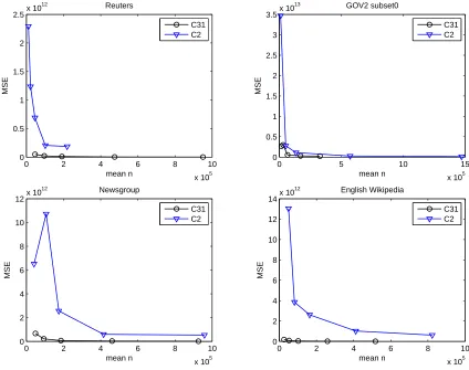
example, if we obtain 100 estimations of GOV2 subset0 collection with each estimation
uses 50 random Webster words, RSD=1.0415. We plot the estimated sizes in Figure 4.1. In
this figure, the red line is the average of 100 estimates. The average estimated size of GOV2
subset0 collection is 1,251,629. However, an estimate could reach 67,338 or 8,430,879. In
English Wikipedia plot, the RSD=0.2205, it can be seen from the plot that the estimated
sizes are gathered relatively in a much more narrow area. Although using 1000 words to
estimate the size English Wikipedia corpus has lower variance, the cost is high according
to Table 4.3.
0 20 40 60 80 100
0 1 2 3 4 5 6 7 8
9x 10
6
GOV2 subset0 Average
0 20 40 60 80 100
0 1 2 3 4 5 6 7 8
9x 10
6
English Wikipedia Average
Figure 4.1: Scatter plot of 100 estimations method C1. For GOV2 subset0, 100 words are randomly selected from the 40,000 Webster words, RSD=1.0415. For English Wikipedia, 1000 words are randomly selected from the 40,000 Webster words, RSD=0.2205.
The large variance is caused by the variation of the query weights. Figure 4.2 depicts
the weight distribution overdf of the corpora under investigation. It shows that queries with
similardfs have small variations in query weights.
Based on this observation, Broder et al. proposed to construct one of the query pools
1 10 100 1000 10000 100000 100000010000000 0.0001 0.001 0.01 0.1 1 10 100 1000 10000 100000 document frequency
weight of terms
English Wikipedia
1 10 100 1000 10000 100000 1000000 0.001 0.01 0.1 1 10 100 1000 10000 100000 document frequency
weight ofa term
Reuters
1 10 100 1000 10000 100000 100000010000000 0.0001 0.001 0.01 0.1 1 10 100 1000 10000 document frequency
weight of terms
Newsgroup
1 10 100 1000 10000 100000 1000000 0.0001 0.001 0.01 0.1 1 10 100 1000 10000 document frequency
weight of terms
GOV2 subset0
the documents as demonstrated in Table 4.12. In addition, they extracted all the terms
from a collection to calculatedf. Although this approach works well when the entire data
collection is available for lexical analysis, it is not possible to obtain such knowledge ofdf
when estimating a data collection with a query interface. Hence, we need to learn the df
information from other sources.
4.3
Constructing a query pool
We propose two ways to construct a query pool, either from another existing corpus that is
completely available to download, or from a sample of the collection whose size is being
estimated.
More formally, given a data collectionD0, which can be a sample of data collectionD,
or some other data collections, our task is to construct a set of terms fromD0such that:
1. The queries in the query pool should have lowdf in data collectionD.
2. The queries in the query pool should cover most of the documents in data collection
D.
Subgoals 1) and 2) contradict each other. When the df is low, it is not easy to cover
most of the documents. Table 4.12 demonstrated this problem. Contrary to this, it will be
too costly to use a query pool with high df queries. We need to select an appropriate df
range so that both 1) and 2) can be satisfied. In the following sections, we show how we
construct query pools from a corpus that is available to download, and from a sample of the
collection.
In general, there are three parameters should be considered when constructing a query
The size of the sample ofD We reported that a sample of 3,000 documents is good enough
to representDin [31]. However, it can be changed based on different situations.
Startingd f Using queries with lowd f will guarantee low variance of query weights and
n. In the real application, it could start with the lowest d f to collect queries from a
sample if the number of queries is not an important factor.
Coverage of the sample Coverage of the sample directly relates to the bias of an
esti-mate. There is no fixed relation between them reported. In the real application of this
method, if 0.02 of RB is acceptable, then the coverage of the sample could be set to
98%.
In our experiments, we choose different settings of the parameters when building a
query pool. These settings are denoted in Table 4.4, which are explained in the later
sec-tions. The terms we extracted from a document are tokenized by Lucene using its default
StandardAnalyzerclass.
Table 4.4: The notations of Pool-based Coverage Method. The sample size is 3000 for C3X.
Notation Approach Settings
C1 Using random words from Webster
-C2 Using low frequency terms from a corpus d f ≥1,coverage=0.995 C31 Using low frequency terms from a sample d f ≥2,coverage=0.995
C32 d f ≥1,coverage=0.95
4.3.1
Learning the query pool from another existing corpus (C2)
In this section we study the approach that learns the queries from another existing data
the query pool by Reuters corpus. This approach is denoted by C2. The construction starts
with extracting all the terms from Retuers corpus and sorts them by theirdfs in ascending
order. We eliminate terms withd f =1 and start to collect terms until they can cover 99.5%
of Reuters corpus. There are 40,340 queries selected from the terms of Rueters corpus.
Table 4.5 records the information of this query pool. Comparing the query pools in C1
and C2 as tabulated in Table 4.2 and Table 4.5, we can see that the learning process of C2
reduces the average number of document the queries can match, which is represented by
the ‘mean d f’. But the variance of weights increases. This is because there are a large
number of common words in Webster. Their weights are in a more narrow range. The
queries selected by C2 need to cover 99.5% of Retuers. Hence, their overall weight range
is larger. This also indicates that the estimation by C32 will not have a lower variance than
C1 according to the statistical data.
Table 4.5: The statistical data of the query pool for C2. The query pool has 40,340 queries.
English Reuters GOV2 subset0 Newsgroup Wikipedia
Coverage ofD 99.5% 99.9% 99.9% 99.9%
max df 185570 474991 882129 691172
min df 1 0 0 0
mean df 217 879 911 827
df RSD 12.9602 10.0205 13.6673 11.7910
max weight 26486.88 20681.30 44009.47 48981.93
min weight 0.0010 0 0 0
W(QP,D) 19.9067 26.6720 34.0120 36.5499
weight SD 281.9400 315.0866 520.7704 511.6770
weight RSD 14.2345 11.8137 15.3114 13.9994
When the query pool is built, we use it to run Algorithm 1 on four English corpora.
Ta-ble 4.6 shows the estimation result. It indicates that this approach produces similar accuracy
docu-Table 4.6: The estimation by C2 on five English corpora. Data are obtained by 100 trials, each trial is produced by randomly selectingt number of queries fromQP.
Corpus Metric t
50 100 200 500 1000 Reuters mean n 11,240 22,246 46,167 101,886 219,259 RB 0.0382 -0.0055 0.0461 -0.0607 0.0008 RSD 1.8073 1.3852 0.9833 0.5944 0.5351 GOV2 subset0 mean n 39,568 79,107 172,080 383,080 823,430 RB -0.1150 -0.1113 0.0189 -0.1539 -0.0855 RSD 2.0989 1.3048 0.8247 0.4918 0.3780 Newsgroup mean n 41,378 106,790 174,700 415,589 958,693 RB -0.1099 0.2167 -0.0329 -0.1027 0.0655 RSD 2.0868 1.9520 1.2049 0.6151 0.4946 English Wikipedia mean n 49,972 81,719 163,632 411,691 823,085 RB 0.2413 -0.0195 0.0062 -0.0118 0.0070 RSD 1.9624 1.3567 1.0874 0.6930 0.5292
ments to produce RB=-0.0329 when estimating the size of Newsgroup collection. However,
C1 needs to check around 300k documents to achieve similar RB.
We visualize the data from Table 4.3 and Table 4.6 in Figure 4.3. It shows that C2
can produce low MSE when the cost is similar to C1 in general. Since C1 produces large
variance and high cost as shown in Table 4.3, the use of random words from a dictionary
should be discarded in this method.
4.3.2
Learning the query pool from a sample of
D
(C3)
In this section, we explore learning a query pool from a sample of D. In section 4.3 we
discuss there are three parameters need to be considered when learning a query pool from
a sample ofD. The constructing process is demonstrated in Algorithm 2.
We choose two settings of the parameters which are denoted by C31 and C32. In [31]
0 1 2 3 4 5 6 7
x 105 0
0.5 1 1.5 2 2.5x 10
12 mean n MSE Reuters C1 C2
0 0.5 1 1.5 2 2.5
x 106 0 0.5 1 1.5 2 2.5
3x 10
12 mean n MSE GOV2 subset0 C1 C2
0 0.5 1 1.5 2 2.5 3 3.5
x 106 0 1 2 3 4 5 6 7x 10
12 mean n MSE Newsgroup C1 C2
0 0.5 1 1.5 2 2.5
x 106 0 0.5 1 1.5 2 2.5 3 3.5
4x 10
12 mean n MSE English Wikipedia C1 C2
Algorithm 2: The construction of a query pool by C3
Input: A dictionaryDic, a data collectionD, the size of the samples, the starting document frequencyd finit and the coverage of the sample p.
Output: ConstructQP.
1. Randomly select a word fromDic;
2. Send the word toDand download all the matched documents toD0.
3. Repeat 1 and 2 untilsnumber of documents are downloaded.
4. Extract all the terms inD0and sort them byd f inD0in ascending order.
5. Remove the terms withd f <d finit.
6. Start with the first one, collect and send the terms one by one toD0and collect all the matched document IDs until p×sdistinct IDs are collected.
7. Save all the collected terms inQP.
from 2 to 0.2× |D0|could cover 99.5% ofD. Hence, we sets=3000 for C3.
C31
We choosed finit =2 and p=99.5% for the initial settings of C3. The size of the QPfor
each of the corpora and theQP’s coverage of Dis recorded in Table 4.7. It also has other
information of the query pools for four collections.
From the statistical data in Table 4.7 and Table 4.5 we can see that queries selected by
C31 have much smaller RSD of query weights than that of C2. This indicates learning
queries from a sample can reduce the variance of estimation.
We run Algorithm 1 using the query pool constructed by C31 on four English corpora.
The results are shown in Table 4.8.
Comparing Table 4.8 with Table 4.3, we can see that using low frequency terms from a
Table 4.7: The statistical data of the query pool of C31.
English Reuters GOV2 subset0 Newsgroup Wikipedia
|QP| 10,847 74,399 17,016 38,853
Coverage ofD 98.90% 99.89% 99.10% 99.01%
max df 20676 82144 66243 31228
min df 2 2 2 2
mean df 951 147 929 517
df RSD 1.3219 0.6440 2.5506 0.1358
max weight 4339.4 6781.75 15171.15 3122.23
min weight 0.02 0.001 0.001 0.001
W(QP,D) 73.6374 14.4190 79.9570 37.5847
weight SD 122.9127 189.2918 225.0074 70.1633
weight RSD 1.6691 13.1279 2.8141 1.8668
Table 4.8: The estimation by C31 on four English corpora. Data are obtained by 100 trials, each trial is produced by randomly selectingt number of queries fromQP.
Corpus Metric t
to check around 500 thousand documents, while 100 queries have already resulted in more
than 700 thousand documents being checked for three corpora using randomly words. Also,
the variance declined as much as 10 times except for the GOV2 subset0 collection. C31 has
successfully reduced the variance of weights except for GOV2 subset0. Take Reuters for
instance, the RSD of weights of random words for C1 is 10.9738, the RSD of the query
pool selected by C31 is 1.6691. The less variance of a query pool, the smaller variation of
the estimation.
0 2 4 6 8 10
x 105 0
0.5 1 1.5 2 2.5x 10
12 mean n MSE Reuters C31 C2
0 5 10 15
x 105 0 0.5 1 1.5 2 2.5 3 3.5x 10
13 mean n MSE GOV2 subset0 C31 C2
0 2 4 6 8 10
x 105 0 2 4 6 8 10
12x 10
12 mean n MSE Newsgroup C31 C2
0 2 4 6 8 10
x 105 0 2 4 6 8 10 12
14x 10
12 mean n MSE English Wikipedia C31 C2
Figure 4.4: A comparison between C2 and C31. The data are from Table 4.6 and Table 4.8.
We visualize the data from Table 4.6 and Table 4.8 in Figure 4.4. It shows that C31 is
C32
We examine if the cost of C31 could be further reduced by choosing another set of values
for the parameters. Although C31 can produce RB< 0.1 for almost all corpora, the cost
is high according to Table 4.8. For example, using 500 queries to estimate the size of
Reuters corpus, it needs to check around 2/3 of the documents that Reuters has. Therefore,
we decrease p to 95%. As the coverage is changed, in order to maintain low variance,
we change thed finit from 2 to 1. We build a query pool for each corpus using above the
settings.
Table 4.9 presents the information of the query pools for four collections. Figure 4.6
and Figure 4.7 present theweight−d f distribution of queries selected by C32 and random words. They show that d fs and weights of queries learnt by C32 are in a more narrow
ranges than those of random words. It means the cost and variance are successfully reduced.
By comparing the statistical data of the query pools for C31 and C32, we can observe that
the cost can be further reduced by C32 except for Newsgroup corpus. However, the variance
of estimation can not be lower because the RSD of weights are higher than those of C31 for
almost all collection. The experimental data of C32 are recorded in Table 4.10 and Table
4.11.
C32 tries to further reduce the cost of C31 by sacrificing some accuracy. Figure 4.5
depicts the performance of C31 and C32.
Figure 4.5 proves that C32 successfully reduces the cost when estimating Reuters,
GOV2 subset0 and English Wikipeida. And it is able to produce lower bias and variance
than C31. However, when C32 estimates the size of English Wikipedia corpus, the bias is
Table 4.9: The statistical data of the query pool of C32.
English Reuters GOV2 subset0 Newsgroup Wikipedia
|QP| 20,862 117,101 40,038 45,449
Coverage ofD 95.60% 94.68% 99.8% 84.76%
max df 24758 51432 119457 6821
min df 1 1 1 1
mean df 228 79 1042 77
df RSD 2.9443 1.8635 2.3966 0.8477
max weight 7799.26 16913.84 2325.06 2387.61
min weight 0.01 0.001 0.0006 0.002
W(QP,D) 36.9721 8.6577 14.6051 23.3278
weight SD 139.6667 185.5397 33.4347 93.1826
weight RSD 3.7776 21.4305 2.2892 3.9945
Table 4.10: The estimation by C32 on five large English corpora. Data are obtained by 100 trials, each trial is produced by randomly selectingt number of queries fromQP.
Corpus Metric t
Table 4.11: The estimation by C32 on small English corpora. Data are obtained by 100 trials, each trial is produced by randomly selectingt number of queries fromQP.
Corpus Metric t
0 2 4 6 8 10 x 105 0 1 2 3 4 5 6 7 8x 10
10 mean n MSE Reuters C31 C32
0 0.5 1 1.5 2 2.5 3 3.5 x 10⁵ 0 0.5 1 1.5 2 2.5 3 3.5x 10
12 mean n MSE GOV2 subset0 C31 C32
0 2 4 6 8 10
x 105 0 1 2 3 4 5 6 7 8x 10
11 mean n MSE Newsgroup C31 C32
0 1 2 3 4 5 6
x 105 0
1 2 3 4 5x 10
11 mean n MSE English Wikipedia C31 C32
4.4
Summary
Generally, Figure 4.3, Figure 4.4 and Figure 4.5 show that C3 is more cost effective and C2
and C1 because it produces lower MSE and checks less documents. And C32 is slightly
better than C31 in terms of the cost. The parameters make this method adjustable and
flexible to estimate the size of an actual deep web data source. As we proved, using a
sample ofD to collect terms will result in the best estimation. In Chapter 5, we compare
C32 with the other three existing methods.
Table 4.12: Coverage of queries when query document frequencies are smaller then a cer-tain value. Queries are from Webster dictionary. It shows that rarer words can not cover all the data source.
d f <100 d f <200 d f <400 d f <800 English Wikipedia queries 15225 18738 22206 25427 coverage 260874 446237 689076 946498 Reuters queries 11739 13540 15101 16434 coverage 165263 261102 374189 493587 GOV2 subset0 queries 16608 19401 21816 24086 coverage 154577 234059 322663 427560 Newsgroup queries 12023 14660 17322 19935 coverage 213705 386514 625135 890285
d f <1600 d f <3200 d f <6400 d f <12800 English Wikipedia queries 28133 30436 32219 33489 coverage 1161432 1316559 1408958 1453897 Reuters queries 17465 18322 18989 19458 coverage 601011 691837 749629 786651 GOV2 subset0 queries 25914 27376 28556 29432 coverage 531493 608433 680575 750637 Newsgroup queries 22271 24339 25854 27037 coverage 1105133 1239541 1295432 1368686
Table 4.13: The statistical data of query pools of C1, C2, C31 and C32.
English Method Reuters GOV2 subset0 Newsgroup Wikipedia
C1 max df 806791 696878 1165272 1066195
min df 0 0 0 0
mean df 1283 4399 5770 4511
df RSD 8.5555 5.5950 6.2986 5.5338
max weight 22003.45 8724.58 8967.26 12202.55
min weight 0 0 0 0
W(QP,D) 20.1703 26.9230 34.3247 36.8789
weight SD 221.3443 190.3310 237.2438 236.2848
weight RSD 10.9738 7.0695 6.9118 6.4069
C2 max df 185570 474991 882129 691172
min df 1 0 0 0
mean df 217 879 911 827
df RSD 12.9602 10.0205 13.6673 11.7910
max weight 26486.88 20681.30 44009.47 48981.93
min weight 0.0010 0 0 0
W(QP,D) 19.9067 26.6720 34.0120 36.5499
weight SD 281.9400 315.0866 520.7704 511.6770
weight RSD 14.2345 11.8137 15.3114 13.9994
C31 max df 20676 82144 66243 31228
min df 2 2 2 2
mean df 951 147 929 517
df RSD 1.3219 0.6440 2.5506 0.1358
max weight 4339.4 6781.75 15171.15 3122.23
min weight 0.02 0.001 0.001 0.001
W(QP,D) 73.6374 14.4190 79.9570 37.5847
weight SD 122.9127 189.2918 225.0074 70.1633
weight RSD 1.6691 13.1279 2.8141 1.8668
C32 max df 24758 51432 119457 6821
min df 1 1 1 1
mean df 228 79 1042 77
df RSD 2.9443 1.8635 2.3966 0.8477
max weight 7799.26 16913.84 2325.06 2387.61
min weight 0.01 0.001 0.0006 0.002
W(QP,D) 36.9721 8.6577 14.6051 23.3278
weight SD 139.6667 185.5397 33.4347 93.1826
The Comparison
This chapter compares the Coverage Method (C32) with several existing methods,
includ-ing the CH-Reg method, Broder’s method, the OR Method. Each method has its own
restriction(s) to choose queries and process returned documents as stated in Chapter 2. In
this chapter, we describe the experiments of the CH-Reg method, Broder’s method and the
OR Method.
5.1
The experiment of the CH-Reg Method
In our experiments, we use a query pool of 40,000 words randomly selected from the
Web-ster Dictionary for the English corpora. In each experiment, the conditions are the same
as those reported in [40], i.e., 5000 words are randomly selected from this query pool,
ig-noring the queries that match less than 20 documents, and take only the top 10 matched
documents for estimation. The results are tabulated in Table 5.1.
We can draw a few conclusions from Table 5.1: i) Estimating the corpora which are
larger than 500k has a larger bias than estimating smaller ones. ii) This method fails to
Table 5.1: A summary of the CH-Reg Method experiment on English corpora. Cells marked by ‘-’ mean data are not available. Each trial randomly selects 5,000 queries the Webster Dictionary and discards any query that returns less than 20 documents. In each query, only top 10 matched documents are returned.
work when estimating the size of GOV2. iii) Because 5,000 queries are issued in each trial,
this method has a low variance, i.e., estimates on almost all the corpora have RB<0.12,
meaning this method has a low variance.
5.2
The experiments of Broder’s method
In the experiments, we choose all 5-digit numbers as the first query pool (QPA). Broder et
al. constructed the second query pool (QPB) by examining the corpus index directly. In our
experiments, we repeat their way of constructing the second query pool, which consists of
the medium frequency terms from each corpus index. Using this approach to constructing
a query pool is impractical in the real-life application. We improve the construction using
a similar approach to C32, i.e., issue random words from the Webster Dictionary, collect
3000 documents and extract terms from the sample to beQPB. Two versions of Broder’s
method are denoted in Table 5.2.
Table 5.2: Broder’s method notations
Notation Dis transparent
B0 0−No
B1 1−Yes
5.2.1
Constructing
QP
Bby terms from
D
Broder’s approach to constructing the second query pool (QPB) requires to scan the corpus
index and extract all terms and theirdf in the corpus. As the first query pool is all 5-digit
numbers, in order to reduce the correlation of two query pools, when building the second
query pool, we discard the terms containing any digits. After extraction, we sort the terms
consecutive terms such that these terms can capture about 30% of the corpus. In this way,
we obtain the second query pool for each corpus. Table 5.3 records the coverage of each
corpus. Tables 5.4 records the experimental data.
Table 5.3: The coverage of medium frequency terms of its corpus
Corpus Reuters English Wikipedia Newsgroup GOV2 subset0
Coverage 30.80% 36.48% 27.79% 30.45%
Table 5.4: Estimation using Broder’s method - B1. RB and RSD are calculated by 100 trials.
Corpus Metric t = 5-digit numbers + medium frequency terms
200 1000 2000 4000 5000 Reuters mean n 655 3,207 6,406 12,801 16,093 RB 0.6559 0.2778 0.2665 0.2424 0.2659 RSD 0.7608 0.2637 0.1868 0.1446 0.1661 English Wikipedia mean n 1,343 6,788 13,560 27,019 33,800 RB -0.3737 -0.3849 -0.3833 -0.3842 -0.3831 RSD 0.0993 0.0145 0.0113 0.0080 0.0066 Newsgroup mean n 1,004 5,075 10,178 20,265 5,067 RB -0.1349 -0.2844 -0.3373 -0.2861 -0.2281 RSD 1.2387 0.6320 0.4176 0.3536 0.7169 GOV2 Subset0 mean n 2,365 12,818 27,258 51,704 62,901 RB -0.5010 0.0450 1.4174 -0.1302 -0.3242 RSD 1.6313 4.0101 5.5971 1.6627 1.3089
The reason why it uses a set of medium frequency terms from the corpus but not random
words is that: A few high frequency words could capture a set of documents that have a
high coverage of the corpus, often as high as 95% as shown in Table 4.3, which makes
|M(QPB,D)|very close toN. The other drawback is that only a few words have high weight
of terms. When randomly selecting words from this kind of query pool, if those high-weight
terms are selected, it would bring a large variance when estimating|M(QPB,D)|. This is
from Webster dictionary. Even randomly selecting 500 queries from each query pool, the
ˆ
|M(QPA,D)∩M(QPB,D)| is always equals to |M(QPˆA,D)|. This means that M(QPB,D)
has already includedM(QPA,D), makingQPA useless.
5.2.2
Constructing
QP
Bby terms from a sample of
D
In this section, we use a query pool learnt from a sample ofDinstead of consideringDis
transparent. The reason is that in the real application, usually a corpus or a data collection
is considered as a black box. It is impossible to obtain the d f of terms in advance. As
we discussed in Section 4.4, learning queries from a sample of D has to configure three
parameters:
• In order to make it comparable with C32, we chose a sample size at 3,000.
• For the startingd f, we also set it to 1 to maintain a low variance.
• Because M(QPB,D) can not be too large as stated in the last section, we set the
coverage to 40%.
The experimental data are recorded in Table 5.5.
5.2.3
Summary
We summarize B0 and B1 in this section. As we can observe from Table 5.4 and Table 5.5,
B0 needs to sample more documents. This is because QPB are not low frequency words
although they have lowd f in the sample ofD. Figure 5.1 shows a comparison between B1
and B0 in MSE-Cost plots.
Figure 5.1 demonstrates B1 can estimate the size of four English corpora more
0 2 4 6 8
x 104 0
1 2 3 4
5x 10
12 mean n MSE Reuters B0 B1
0 1 2 3 4 5
x 105 0
1 2 3
4x 10
12 mean n MSE GOV2 subset0 B0 B1
0 5 10 15
x 105 0 1 2 3 4 5 6
7x 10
11 mean n MSE Newsgroup B0 B1
0 1 2 3 4 5 6
x 104 3 3.5 4 4.5 5 5.5 6
6.5x 10
11 mean n MSE English Wikipedia B0 B1
Table 5.5: Estimation using Broder’s method - B0. RB and RSD are calculated by 100 trials.
Corpus Metric t = 5-digit numbers + medium frequency terms
50 100 200 1000 2000 Reuters mean n 4,724 15,815 76,514 151,000 301,400 RB 0.1653 -0.3531 -0.3916 -0.3996 -0.4032 RSD 2.1759 0.4642 0.1295 0.0710 0.0591 GOV2 subset0 mean n 4,539 8,781 14,866 81,472 161,498 RB -0.3772 -0.4439 -0.5401 -0.4340 -0.1726 RSD 1.3691 1.4593 0.5714 0.5138 2.1090 Newsgroup mean n 16,508 31,144 65,475 314,656 629,839 RB 6.5787 0.0563 -0.2526 -0.4018 -0.4408 RSD 7.3737 1.8539 0.6939 0.7236 0.4223 English Wikipedia mean n 3,260 5,896 11,644 59,430 121,158 RB -0.4504 -0.5174 -0.5213 -0.5123 -0.5049 RSD 0.4589 0.3176 0.2431 0.1138 0.0805 GOV2 2M mean n 21908 45,497 92,976 454,214 920,182 RB -0.5990 -0.4803 -0.5510 -0.5669 -0.4853 RSD 0.7938 0.9744 0.5278 0.3433 1.5719
size of the GOV2 subset0 seems difficult because the points are spread in a wide range on
they-axis. This is because the variance of the estimates is large. We will discuss why the
estimated size of the GOV2 subsets are varied so much in the later sections.
The reason we are not able to obtain the data of Broder’s method on small collections
is that the estimate of|M(QPA,D)|has a high chance to be 0.
5.3
The experiment of the OR Method
We also carry out experiments to collect data on the OR Method. The query pool used for
estimating the size of English corpora is 40,000 Webster words. In each trial, the top 2% of
Table 5.6: Estimating small English corpora using the OR Method. Bias and standard deviation of the estimation over 100 trials. In each trial, queries are randomly selected from 40,000 Webster words.
Corpus Metric t
Table 5.7: Estimating large English corpora using the OR Method. Bias and standard deviation of the estimation over 100 trials. In each trial, queries are randomly selected from 40,000 Webster words.
Corpus Metric t
5.4
The experiments on Chinese corpora
We experiment the CH-Reg method, the OR method and C32 on Chinese corpora. B0 and
B1 are not easy to implement because it is difficult to choose two uncorrelated query pools
for Chinese corpora. Take the Sogou Web Corpus 500k for example, we tried to query all
5-digit numbers on this collection, but no document matched them.
When carrying out the experiments on Chinese corpora, we need to decide whether the
queries should be single Chinese characters or Chinese phrases for the CH-Reg Method
and OR Method. In general, Chinese characters have much higherd fs than English words
because the number of characters are usually limited to be a few thousands in most corpora.
Thus a few hundreds of random Chinese characters may match most of the documents.
On the other hand, using phrases will reduce the cost because phrases have lowerd f than
characters. The dictionary we used is the Contemporary Chinese Dictionary, which contains
44,905 phrases. Queries selected by the CH-Reg Method and OR Method are phrases.
When creating a sample of a Chinese collection using C32, we use phrases as queries.
After documents are collected by queries, it is difficult to extract all the phrases from a
Chinese document because the Chinese segmentation is still a problem under research.
Hence, the terms collected from a sample ofDare all the terms tokenized by Lucene. By
inspecting the query pools built by C32 from Chinese documents, we found that these terms
consist of not only Chinese characters but also some other symbols in the documents.
The data of the CH-Reg Method, the OR Method and C32 are tabulated in Table 5.8,