Fluid Dynamics of the Evolution of Supernova Remnants and Granular Materials.

ABSTRACT

TANG, ZHU. Fluid Dynamics of the Evolution of Supernova Remnants and Granular Materials. (Under the direction of Karen Daniels.)

My thesis addresses two research fields. For the astrophysics part, we present analytical and numerical studies of models of supernova-remnant (SNR) blast waves expanding into uniform media and interacting with a denser cavity wall, in one spatial dimension. We predict the nonthermal emission from such blast waves: synchrotron emission at radio and X-ray energies, bremsstrahlung, inverse-Compton emission (from cosmic-microwave background seed photons), and emission from the decay ofπ0mesons produced in inelasticcollisions between accelerated ions and thermal gas, at GeV and TeV energies. Accelerated particle spectra are assumed to be power-laws with exponential cutoffs at energies limited by the remnant age or (for electrons, if lower) by radiative losses. We show the dependence of images and spectra on various model parameters. We compare the results with those from homogeneous (“one-zone”) models. Such models give fair representations of the 1-D results for uniform media, but cavity-wall interactions produce effects for which one-zone models are inadequate. We study the time evolution of SNR morphology and emission with time. Strong morphological differences exist between ICCMB andπ0-decay emission; at some stages, the TeV emission can be dominated by the former and the GeV by the latter, resulting in strong energy-dependence of morphology. Integrated gamma-ray spectra show apparent power-laws of slopes that vary with time, but do not indicate the energy distribution of a single population of particles. We compare models to data for the Cygnus Loop supernova remnant. As observational capabilities at GeV and TeV energies improve, spatial inhomogeneity in SNRs will need to be accounted for.

For the granular fluid part, the flow of dense granular materials at low inertial numbers cannot be fully characterized by local rheological models; several nonlocal rheologies have recently been developed to address these shortcomings. To test the efficacy of these models across different packing fractions and shear rates, we perform experiments in a quasi-2D annular shear cell with a fixed outer wall and a rotating inner wall, using photoelastic particles. The apparatus is designed to measure both the stress ratioµ(the ratio of shear to normal stress) and the inertial number I through the use of a torque sensor, laser-cut leaf springs, and particle-tracking. We obtainµ(I) curves for several different packing fractions and rotation rates, and successfully find that a single set of model parameters is able to capture the full range of data collected once we account for frictional drag with the bottom plate. Our measurements confirm the prediction that there is a growing lengthscale at a finite valueµs, associated with a frictional yield criterion. Finally, we newly identify the physical mechanism behind this transition atµs by observing that it corresponds to a drop in the susceptibility to force chain fluctuations.

© Copyright 2018 by Zhu Tang

Fluid Dynamics of the Evolution of Supernova Remnants and Granular Materials

by Zhu Tang

A dissertation submitted to the Graduate Faculty of North Carolina State University

in partial fulfillment of the requirements for the Degree of

Doctor of Philosophy

Physics

Raleigh, North Carolina

2018

APPROVED BY:

Stephen Reynolds Michael Shearer

Edgar Lobaton Hans Hallen

Karen Daniels

DEDICATION

BIOGRAPHY

Zhu Tang was born in Nanjing, China. Nanjing is one of the China’s Four Great Ancient Capitals (Xi’an, Nanjing, Beijing, Luoyang ). Zhu was growing up in the residential buildings built in Republic China period. These buildings combine both the traditional Chinese garden art and the Western architecture art. These beautiful architecture aroused her interest in art. Zhu went to an art middle school (Nanjing Ninghai Middle school) and studied basic art skill and theory for three years.

During her childhood, Zhu was also interested in Science. Her father, a professor in physics department, allowed her to do school homework in his undergraduate physics lab classroom. Then, she had a chance to observe different interesting physics phenomenon every week, and got some easy understanding answers after her questions. Her father also loved doing small science experiments with her, like changing the flour color into blue by adding iodine or creating image by a lens.

When Zhu went to high school (the High School Affiliated to Nanjing Normal University), she enjoyed in learning physics, and joined physics activities. She also participated high school com-petition in physics and got second price of Jiangsu Province twice. Then she determined to study physics in college. In 2007, Zhu went to Northeastern University and studied physics in Liaoning Province of China. She did experiments on superconducting material, looking for the method of creating Bi2212 superconducting material on the NiO substrate.

In 2012, she started the PhD program in North Carolina State University. From August 2013 to August 2015, she worked with Dr. Stephen Reynolds and studied the X-rayγ-ray from middle age supernova remnant. Then she worked with Dr. Karen Daniels and studied the rheology of granular materials.

ACKNOWLEDGEMENTS

TABLE OF CONTENTS

LIST OF TABLES . . . vii

LIST OF FIGURES. . . .viii

Chapter 1 Introduction to fluid mechanics . . . 1

Chapter 2 Introduction to hydrodynamic simulation in supernova remnants . . . 3

2.1 Supernovae . . . 4

2.2 Supernova remnants . . . 6

2.3 Cosmic Rays . . . 7

2.4 Particle acceleration in shock waves . . . 8

2.5 Radiative processes . . . 8

2.6 Simulation model . . . 10

2.6.1 VH-1 hydrodynamic code . . . 11

2.6.2 Supernova remnant model . . . 11

Chapter 3 Simulations of spectra and images of supernova remnants in cavities . . . 13

3.1 Hydrodynamic simulation . . . 14

3.2 Radiation . . . 19

3.3 Conclusion . . . 40

Chapter 4 Introduction to granular flow . . . 41

4.1 Granular media . . . 41

4.1.1 Granular packing . . . 42

4.1.2 Granular flow . . . 43

4.1.3 Different flow regions . . . 45

4.2 Local rheology . . . 48

4.3 Nonlocal rheology . . . 48

4.3.1 Cooperative model . . . 49

4.3.2 Gradient model . . . 50

4.3.3 Other nonlocal models . . . 52

4.4 Nonlocal rheology for particles of different shapes . . . 53

4.5 Motivating Questions . . . 55

Chapter 5 Methods . . . 56

5.1 Introduction . . . 56

5.2 Introduction . . . 57

5.3 Method . . . 59

5.3.1 Apparatus . . . 59

5.3.2 Calibrating the spring wall . . . 59

5.3.3 Measuring wall deformation . . . 59

5.3.4 Measuring wall stresses . . . 62

5.4.1 Stress measurements . . . 62

5.4.2 Rheological measurements . . . 64

5.5 Conclusion . . . 64

Chapter 6 Nonlocal rheology . . . 66

6.1 Abstract . . . 66

6.2 Introduction . . . 67

6.2.1 Cooperative model . . . 68

6.2.2 Gradient model . . . 70

6.3 Method . . . 72

6.3.1 Apparatus . . . 72

6.3.2 Particle tracking . . . 73

6.3.3 Inertial number . . . 76

6.3.4 Shear and normal stress . . . 76

6.4 Results . . . 77

6.4.1 µ(I)rheology . . . 77

6.4.2 Fluidity . . . 79

6.4.3 Comparison to models . . . 80

6.4.4 Nonlocal lengthscale . . . 81

6.4.5 Yield stress ratioµs . . . 83

6.5 Conclusions . . . 85

Chapter 7 The effect of particle shape on nonlocal rheology . . . 87

7.1 Abstract . . . 87

7.2 Introduction . . . 88

7.2.1 Cooperative model . . . 89

7.3 Method . . . 90

7.3.1 Apparatus . . . 90

7.3.2 Calculate speed and shear rate . . . 92

7.3.3 Calculate local packing fraction by Coarse-graining . . . 95

7.4 Results . . . 97

7.4.1 µ(I)results for particles in different shapes . . . 97

7.4.2 Best fitting for different shapes . . . 97

7.4.3 Length scale . . . 99

7.4.4 Microscopic Description of the Granular Fluidity . . . 101

7.5 Conclusions . . . 102

Chapter 8 Conclusion. . . .103

LIST OF TABLES

Table 3.1 Model Parameters: Uniform Medium a: Corresponds to downstream density in all other models. b: Average over obliquities. Upstream fieldB₁is 1.4µG. c: Same as model JB in standard-collision set. (Table 3.2) Models U1, U2, and U3 use the 1-D hydrodynamic simulations. . . 17 Table 3.2 Model Parameters: Standard Collision (Fig. 3.4 to Fig. 3.9) In all cavity models,

the wall is located atRw=2.67×1019cm, with a density jump there of a factor of 20, unless otherwise noted. The collision occurs at a time of about 2000 yr, when the shock velocity is 1690 km s−1_{. a: Density in cavity interior. b: Density} in cavity wall. . . 18 Table 3.3 Parameter table for Fig. 3.11 to Fig. 3.26 . . . 37

Table 6.1 Description of the six datasets. The inner wall rotationv(Ri)is the speed set by the motor controller. The number of particles is set by hand to one of two values (corresponding to 4 runs atΦlo with 5610 particles and 2 runs atΦhiwith 5760 particles). The global packing fractionΦis calculated from number of particles, the area of the particles, and the area of the shear cell (including the measured spring wall dilation). The±values correspond to errors in the measurement of the particle size and the fluctuations in the spring wall dilation; these are of similar magnitude, and were added in quadrature. PressureP is calculated from spatially- and temporally-averaging the normal stress measured at the 52 spring wall arms. The±values are the standard deviation of these measurements across both space (52 arms) and time. The microscopic timescaleT is calculated based on this pressure and known values ofd andρ. . . 72 Table 6.2 Fitting parameters for both models, with±values representing the sensitivity

range. The sensitivity forµs (identical for both models) is taken from the full-width-half-maximum of the peak in the inset to Fig. 6.7. For the four parameters(A,b,`,a), the sensitivity is determined from the run withΦ<sub>hi</sub>and 2d/s by holding one parameter fixed and allowing the residual to vary up to R2=0.3 (rather than the best-fitR2=0.2 shown in Fig. 6.5a). Similarly, for the lengthscale parameterν<sub>`</sub>, the sensitivity range is for an increase fromR2_=0.02 to 0.03 for the data and fit given in Fig. 6.7. . . 80

Table 7.1 Description of the seven datasets. The inner wall rotationv(Ri)is the speed set by the motor controller. The number of particles is set by hand to provide a one of two one of two pressures to within±0.3 kPa. The microscopic timescaleT is calculated based on the pressure and known values ofd andρ. First column is from Tang et al.[Tan18]. . . 92 Table 7.2 Best fitting parametersAandbdifferent particle shapes, with error bars

LIST OF FIGURES

Figure 2.1 Classification of supernovae . . . 5

Figure 2.2 Left: Cygnus Loop (X-ray; ROSAT) (NASA/GSFC). Right: Cassiopeia A. Red: infrared, orange: visible; blue: X-Ray . . . 6

Figure 2.3 The model of synchrotron radiation . . . 9

Figure 2.4 The model of Inverse-Compton radiation . . . 9

Figure 2.5 The model of Bremsstrahlung radiation . . . 10

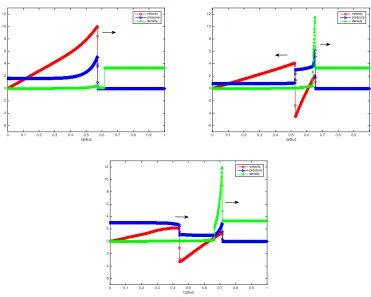
Figure 3.1 The velocity is in red circles. The pressure is in blue triangles. The density is in green stars. Top left: The shock wave just before hitting the wall. Top right: The speed, density, and pressure profile of the cavity when the shock wave has passed the density jump, with part of the wave reflected. Bottom: Later time, showing the speed, density, and pressure profile of the cavity when the shock wave has moved further into the wall, and part of the wave has reflected from the center. . . 14

Figure 3.2 Four snapshots of the blast wave just after reaching the wall where the density jumps by a factor of 20. The times are 2070, 2210, 2650, and 3530 yr. Densities are in units of 4×10−23cm−3, pressures in units of 4×10−8dyn cm−2, and velocities in units of 1000 km s−1. Note the scale change between the third and fourth panels. The reflected shock accelerates rapidly back toward the remnant center. . . 15

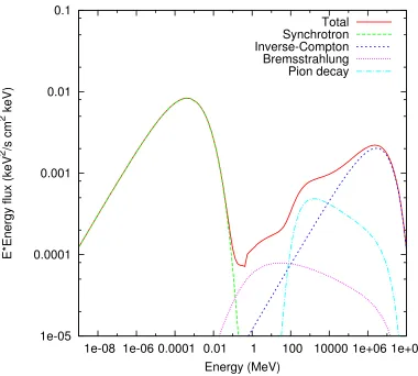
Figure 3.3 Emissivities for the four principal processes producing X-ray to gamma-ray emission. Parameters are shown in Table 3.1. . . 18

Figure 3.4 Spectra as a function of time, for the standard collision model. (a) JB (just before; age 1700 yr); (b) model A1 (2027 yr); (c) model A2 (2236 yr); (d) model A3 (2740 yr); (e) model A4 (3541 yr); (f ) model A5 (5350 yr). Note the change in relative strengths of IC andπ0-decay processes with time, causing dramatic changes in the summed spectrum at GeV to TeV energies. . . 20

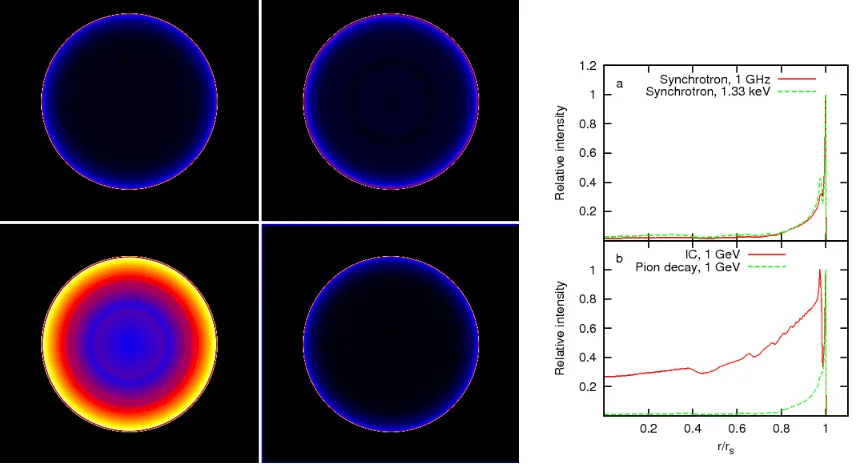
Figure 3.5 Images and profiles due to different radiative processes, for model A1. Top row: Synchrotron emission at 1 GHz and 1.33 keV, and profiles (a). Bottom row: IC andπ0emission at 1 GeV, and profiles (b). The images and profiles for IC andπ0_{emission at 1 TeV are indistinguishable from those at 1 GeV, and} the bremsstrahlung image is very similar to theπ0-decay image throughout. The color scale is relative to each image maximum. . . 21

Figure 3.6 Images and profiles due to different radiative processes, for model A2. Top row: Synchrotron emission at 1 GHz and 1.33 keV, and profiles (a). Bottom row: IC andπ0emission at 1 GeV, and profiles (b) (indistinguishable from those at 1 TeV). The small ripples in the IC image are artifacts of the numerical interpolations. Again, the color scale is relative to each image maximum. . . . 22

Figure 3.8 Images and profiles due to different radiative processes, for model A4. Top row: Synchrotron emission at 1 GHz and 1.33 keV, and profiles (a). Middle row: IC andπ0emission at 1 GeV, and profiles (b). Bottom row: IC andπ0 emission at 1 TeV, and profiles (c). . . 24 Figure 3.9 Images and profiles due to different radiative processes, for model A5. Top

row: Synchrotron emission at 1 GHz and 1.33 keV, and profiles (a). Middle row: IC andπ0emission at 1 GeV, and profiles (b). Bottom row: IC andπ0emission at 1 TeV, and profiles (c). The bump nearr/rs=0.5 for IC emission at 1 TeV is an artifact of the numerical interpolations, visible only at the highest energies. 25 Figure 3.10 Comparison of the integrated spectrum of model A3 with that from a

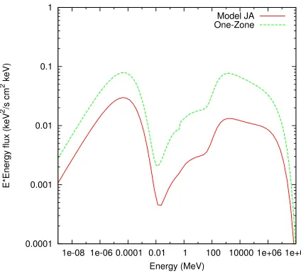
homo-geneous (one-zone) model using the parameters of the forward blast wave (in the dense medium). . . 26 Figure 3.11 The radiation fluxes for different radiation processes at 4.15×10−9keV, 1.33 keV,

1.33×106_{keV, and 1.33×10}9_{keV for cavity structure. . . 27} Figure 3.12 The radiation fluxes for different radiation processes at 4.15×10−9keV, 1.33 keV,

1.33×106keV, and 1.33×109keV for uniform case. . . 28 Figure 3.13 The age at 1700, 2700 (time hitting the wall), 5400, 20000, and 54000 year

simulation spectrum. . . 29 Figure 3.14 fB=6.67×10−6 . . . 30 Figure 3.15 fB=2.0×10−6 . . . 30 Figure 3.16 First line: Synchrotron at 4.15×10−9keV. Second line: Synchrotron at 1.33 keV.

Third line: Inverse Compton scattering (red), Bremsstrahlung (green) and π0_{-Decay (blue) at 1.33×10}6_{keV . Fourth line: Inverse Compton scattering} (red), Bremsstrahlung (green) andπ0-Decay (blue) at 1.33×109keV. Left :

fB=6.67×10−6, Right:fB=2.0×10−6 . . . 31 Figure 3.17 Density jump of 20 at cavity wall, s=2.2 . . . 32 Figure 3.18 Density jump of 50 at cavity wall, s=2.2 . . . 32 Figure 3.19 First line: Synchrotron at 4.15×10−9keV. Second line: Synchrotron at 1.33 keV.

Third line:Inverse Compton scattering (red), Bremsstrahlung (green) andπ0 -Decay (blue) at 1.33×106_{keV . Fourth line: Inverse Compton scattering (red),} bremsstrahlung (green) andπ0-Decay (blue) at 1.33×109keV. Density jump Left : 20, Right: 50 . . . 33 Figure 3.20 s=2.2 . . . 34 Figure 3.21 s=2.0 . . . 34 Figure 3.22 First line: Synchrotron at 0.415×10−8keV. Second line: Synchrotron at 1.33 keV.

Figure 3.25 First line: Synchrotron at 0.415×10−8keV. Second line: Synchrotron at 1.33 keV. Third line:Inverse Compton scattering (red), Bremsstrahlung (green) andπ0 -Decay (blue) at 1.33×106keV. Fourth line: Inverse Compton scattering (red), Bremsstrahlung (green) andπ0-Decay (blue) at 1.33×109keV. Left : Gyrofactor η=100, Right:η=10 . . . 38 Figure 3.26 Example of a model providing a fairly good description of the Cygnus Loop

(data points). Age 9118.7 years, current shock speed 341 km/s, cavity density 1.17 x 10−25_{g cm}−3_{, density jump a factor of 28, f}

b =7 x 107, s=2.2, and gyrofactorη=100. This model explains the GeV emission as due toπ0 de-cay, and requires a very low ratio of electrons to ions, kei=0.0005, to avoid overproducing radio synchrotron emission compared to gamma rays. . . 39

Figure 4.1 Different kinds of granular media[And13] . . . 42 Figure 4.2 The variables for the granular flow in the example of plane shearing.P is the

pressure in the granular media,τis the shear stress,r presents the position coordinate,d is the particle diameter,vis the speed of the particles, and ˙γis the shear rate. . . 44 Figure 4.3 Rheology results in different experiments: (a) and (b) 2D configurations with

disks; (c) and (d) 3D configurations with spheres; (e) and (f ) empirical ana-lytical laws ofµ(I)andφ(I)by fitting experimental and simulation results

[And13]. Data from[Pou99; SS84; DC05; MiD04; Bar06]. . . 45 Figure 4.4 Soild, liquid, and gas flow regions[FP08] . . . 46 Figure 4.5 Six configuration of granular flows: (a) plane shear, (b) annular shear, (c)

vertical-chute flows, (d) inclined plane, (e) heap flow, (f ) rotating drum.[MiD04] 47 Figure 4.6 (a) Inertial numberI in three flow regimes. (b) The force network in two

dimensional shear flow for the three regimes.[And13] . . . 48 Figure 4.7 Example of non-convex particles: Each star consists of six orthogonal square

beams[Zha16]. . . 53 Figure 4.8 The contact between particles for three different shapes: (a) side to side

con-tact (a’) limiting case for side to side concon-tact (b) vertex to side concon-tact concon-tact (b’) limiting case for vertex to side contact (c) three pentagons vertices contact (d) and (e) round particles contact[Dup95] . . . 54 Figure 4.9 Normal forces in disks (a) and pentagons (b). Line thickness is proportional

to the normal force[Azé09a]. . . 54

Figure 5.1 Top view of annular Couette experiment with≈5000 disk-shaped particles confined between a rough inner ring of radiusRi=15 cm and a segmented outer ring of radiusRo=28 cm. Each of the leaf springs which make up the outer ring can allow dilation under stresses imposed by the dilating granular material. . . 58 Figure 5.2 (a) Photograph of a single leaf spring mounted in the Instron for calibration,

Figure 5.3 Closeup images of the spring tip with (a) and without (b) particles, and these same tips isolated using image-processing (c,d). (e) The contour plot for of cross-correlation values between images (c,d), with the maximum value corresponding to the(d x,d y)displacement. . . 61 Figure 5.4 (a) Time series of normal and tangential stresses for a single leaf spring, Case

1 experiment. (b) Time-average normal and tangential stress and standard error for all three cases by one sensor. . . 63 Figure 5.5 Sampleµ(I)curves for all 3 cases. . . 65

Figure 6.1 Top view of annular Couette experiment with≈5000 flat photoelastic particles. Image is a composite of an image of the leaf springs and an image of the force chains, inverted for clarity (light particles are those experiencing more force). The inner wheel (R_i=15.0 cm=26.8d) rotates at fixed speed, and the stationary outer boundary (Ro=28.0 cm=50.0d) is composed of 52 laser-cut leaf springs. The tips of the leaf springs are calibrated to measure shear (τ) and normal (P) stress. The speed profilev(r)is measured via particle-tracking. 69 Figure 6.2 (a) Speed profilesv(r)and (b) shear rates ˙γfor all six datasets, measured by

particle-tracking. The distance from inner wall is at location∆r=r−Ri. We estimate the error bars using finite differences, and show typical values for one run. Data files for all figures are available online through DataDryad[DOI citation to be added in proof]. . . 74 Figure 6.3 Local packing fraction profilesφ(r), for all six datasets. The solid line is an

exponential with decay lengthr0= (1.67±0.17)d, taken from averaging over fits to all six datasets. . . 75 Figure 6.4 Modeled shear stress profiles τ(r), determined from the model given in

Eq. 7.10, with τ0= (250±30)Pa and r0 taken from Fig. 6.3. Datapoints at Ricome from the torque sensor, and atRo from the leaf springs, for each of the six datasets. . . 76 Figure 6.5 (a) Stress ratioµas a function of inertial numberI, for all six datasets. The

hor-izontal dotted line indicates the location ofµs=0.26 to distinguish the local (upper) and nonlocal (lower) regions. Speed profilesv(r)for all six datasets, plotted as (b) raw data on a linear axis and (c) normalized on a logarithmic axis. In all cases, solid lines compare to the cooperative model (§7.2.1) and dashed lines to the gradient model (§6.2.2). For comparison, we calculate relative residuals asR2≡ 〈(aexp−ath)2/(aexp2 )〉, with the average taken over all data points. For (a):R2_{=0.204 for the cooperative model, andR}2_=0.210 for the gradient model. For (b,c):R2=0.129 for the cooperative model, and R2_{=0.124 for the gradient model. . . 78} Figure 6.6 Experimentally-measured granular fluidity (calculated by Eq. 6.18 and Eq. 6.19),

Figure 6.7 (a) Speed profile v(r)for the dataset withΦhiand rotation rate 2d/s. The dash-dotted line is given by a fit to Eq. 6.20 withα3=−0.0118,α2=−0.1096, α1=−0.8374, andα0=0.6512, using the filled data points (aboveµs). (b) Comparison of the measured lengthscale (blue) to the two models (black), scaled by particle diameterd. Both of the models have a divergence near the value µs =0.26, as expected from Fig. 6.5a. For µ > µs (local regime), the relative residuals areR2=0.053 for the cooperative model (black solid line) andR2_{=0.092 for the gradient model (black dashed line), based on a} comparison with the analytic derivative (blue dash-dotted line). Forµ < µs (nonlocal regime), these same residuals are quite large:R2=1.617 for the gradient model,R2_{=3.819 for the cooperative model. . . 82} Figure 6.8 The variance of the light (force) intensity within concentric rings, plotted

parametrically against the value ofµmeasured within that ring. The sharp drop is atµs=0.29. Inset: Image of force chains, inverted for clarity, so that dark particles are those experiencing more force. Data collected atΦhiand at rotation rate 2d/s. Upper line (magenta) overlays the measuredµ(r)with µs=0.29 marked by the circle. Lower line (green) overlays the measuredv(r) for comparison. . . 84

Figure 7.1 Top: Top view of annular Couette experiment with flat pentagonal particles. Bottom: Photo of the circular/elliptical photoelastic particles, along with the three acrylic shapes: ellipses, circles, and pentagons. The central holes allow for easier particle-tracking. Each of the acrylic particles can be circumscribed by a square of side length 0.7 cm (small particles) or 1.0 cm (large particles). . 91 Figure 7.2 The relationship between the packing fraction and the pressure for different

shapes. In the legend, Vi presents the particle material from Vishay, and Ac presents the particle material is acrylic. Blue triangle data is from[Tan18]. . . 93 Figure 7.3 (a) Speed profilev(r)and the (b) shear rates ˙γfor all the seven data sets. Blue

triangle data is from[Tan18] . . . 94 Figure 7.4 The local packing fraction for different shapes and materials in low pressure is

calculated by coarse-graining method. The solid curves are the corresponding fitting curves from Eq. 7.9. The fitting parameterr0for pentagon is 1.69, for circle is 2.04, for ellipse is 1.28. The circle/ellipse (Vi) data are from[Tan18]. . 95 Figure 7.5 (a) Stress ratioµas a function of inertial numberI, for all seven datasets. (b)

Speed profilesv(r)for all seven datasets. The solid curves are calculated from the cooperative model, using model parameters from Table 7.2. . . 98 Figure 7.6 (a) Speed profile forP_hiparticles in different shapes. The dash-dotted lines

CHAPTER

1

INTRODUCTION TO FLUID MECHANICS

Fluid dynamics aims to solve the problem of the motion of fluids[Lan59]. In this thesis, I will present two examples of the application of fluid dynamics in two different fields. The first one is the use of fluid dynamics in astrophysics by applying well developed hydrodynamic methods to solve the motion of blast waves in supernova remnants. In the second example, novel fluid phenomenon and models for granular media are presented and tested.

We study the flow of granular media and the supernova remnants. However, there are some differences between them. Supernova remnants are composed of ions and we treat them as ideal inviscid compressible gas, which can be described by the Euler Equations. We study the flow from blast waves and predict the speed profiles, density profiles and pressure profiles from the simulation dynamics, where the speed can be as fast as 2000 km per second. In contrast, granular materials are composed of grains, which are less compressible. The compression in granular media, where particles are close to each other, is different from the ideal inviscid compressible gas, where the distance between particles is large enough to ignore the particle size. There are two ways to compress granular media: the first way is by reducing the distance between particles, squeezing more particles into the same space. The second way is by squeezing particles and causing elastic deformation. Thus, the flow of granular media becomes complicated. We need to take into account the state of granular media (gas like, liquid like, or solid like) and the particle properties (shape, stiffness) when we study the granular media flow.

material of supernova remnants is treated as an ideal inviscid compressible gas. We predict the behavior of blast waves in supernova remnants by solving the Euler equations. In Chapter 2 and 3, the basic knowledge of supernova and supernova remnants are introduced. The dynamics of variables, like the density, pressure and speed among the remnants, are calculated through hydrodynamic simulation. The radiation spectrum of the supernova remnants depend on the dynamics of the variables.

CHAPTER

2

INTRODUCTION TO HYDRODYNAMIC

SIMULATION IN SUPERNOVA

REMNANTS

Fluid dynamics has been widely used in different fields. In this chapter, I will focus on the the application of fluid dynamics in the field of astrophysics, especially, the area of supernova remnants (SNR). The study of the radiation in supernova remnants can help us learn about the origins of cosmic rays, and the evolution of supernovae.

2.5.

My work is about the simulation of supernova remnants evolving in a low-density region (cavity) produced by a stellar wind from the progenitor star before the explosion. I assume an ideal case for the model. Firstly, the evolution happens in an ideal inviscid compressible plasma. And it is also adiabatic; the loss of energy from radiation will be neglected. Using this ideal model, some basic values like velocity, pressure and density for calculating the radiation in the future can be determined. According to these basic values, we can calculate the radiation predicted by our models. In this thesis, we will focus on X-rays andγ-rays from the supernova remnants and cosmic rays they produce.

In the following sections, I will introduce the basic information about supernovae, supernova remnants and cosmic rays. In Chapter 3, I will present the research results on simulated images and spectra.

2.1

Supernovae

A star is initially supported against gravity by energy from the nuclear reactions converting H to He in the core. However, it can not stay in a static equilibrium state forever. It will evolve after running out of fuel. After this equilibrium state (main sequence), hydrogen in the inner core will be used up, so the core contracts, and the inner temperature rises. Then hydrogen in a layer outside the core will be ignited. At this stage, the outer layers will expand. So the star will have a large size. We call it the red giant phase. When hydrogen in the core is almost converted into Helium , Helium will be ignited to produce carbon. Then, in massive stars only, carbon will be converted, followed by Neon, and Silicon until the star’s core is mainly iron. The elements left in the core at last depend on the mass of the star. For a low mass star with an initial mass less than eight times the mass of the Sun, the synthesis of heavy elements like iron can not be reached. This kind of star can never reach temperatures and pressures high enough for nuclear fusion up to iron. The lowest mass stars can only ignite Helium. Most stars like our sun can reach to the synthesis of carbon.

Core-collapse is not the only way to obtain a supernova. Through binary interaction, we can get another kind of supernova, a type Ia supernova. In this binary system, one of the stars is a white dwarf, and the other can be any star. The two stars revolve around each other, and the white dwarf absorbs the mass of the other star. When its mass gets to 1.4 solar masses (the Chandrasekhar limit), the white dwarf will no longer be stable, and carbon burning can be ignited explosively, producing a Type Ia supernova. In contrast to core-collapse, the explosion energy is from thermonuclear energy, which is carbon burning and silicon burning.

The observational classification of the supernovae depends on the the spectrum and light curve. Light curves show the light intensity changing with time after the explosion for weeks to months. In Fig, 2.1, we can see the classification scheme. The spectrum of a Type I supernova has no Hydrogen. On the other hand, we can detect Hydrogen in the spectrum of Type II supernovae. A type Ia supernova does not have Hydrogen initially, but we can detect Silicon. For a massive star, stellar winds can remove the outer layers. For Type Ib, Hydrogen is missing and for Type Ic supernova both Hydrogen and Helium are missing. The difference between Type IIL and Type IIP is the light curve. The luminosity of the both kinds increases to a peak then drops. The following phenomenon distinguishes these two types. The Type IIL supernova shows a linear decline after the peak. On the contrary, the Type IIP supernova shows a plateau.

Figure 2.1Classification of supernovae

2.2

Supernova remnants

After an explosion of a massive star, a supernova remnant will be left. In Fig. 2.2, there are two examples of supernova remnants: the Cygnus Loop and Cassiopeia A. Cassiopeia A is one of the youngest SNRs in the galaxy, about 340 years old. The Cygnus Loop is thought to be about 8000 years old.

Figure 2.2Left: Cygnus Loop (X-ray; ROSAT) (NASA/GSFC). Right: Cassiopeia A. Red: infrared, orange: visible; blue: X-Ray

Supernova remnants can be classified by their shapes: shell-like, Crab-type, and composites of these two. In my research, I will focus on those with shell-like structure. The supernova remnants with this kind of structure look like bright rings. Most of them are old. Different from shell remnants, crab-like remnants look more like a blob. The famous Crab Nebula belongs to this kind of structure. Most of them are young supernovae. Composite remnants have both between shell-like and central crab-like components.

• Dynamic evolution of supernova remnants

Supernova remnants will go through different phases.[Dye01]The first phase is free expansion. At the beginning, the pressure in the surroundings can be ignored. An explosion happens in the center of the progenitor star, sending a shock wave through the star and ejecting the outer layers. The structure of the ejected material for both core-collapse and Type Ia supernova is approximately uniform in the center area, and an power-law density decreasing in the outer region.[Rey98]

The following phase is the Sedov-Taylor phase. It can be simulated by a self-similar analytic solution for a point explosion in a uniform medium. The analytic solutions use the variables density, pressure and time. The shock radius can be calculated byRs=1.15(E/ρ)1/5t2/5.[Rey98]This stage can last for hundreds to a few thousand years. Until now the expansion is adiabatic. The hot gas has not had time to cool.

When the shock velocity slows to less than about 200k m/s, the supernova remnant goes to the radiative phase, when cooling becomes important, and the shock compression ratio becomes much larger. We can observe significant visible light at this phase.

The last phase is the shock merging with the interstellar medium. The shock waves will lose their energy, and merge into the surrounding interstellar medium eventually.

2.3

Cosmic Rays

Cosmic rays are high energy charged particles, traveling in space. The speed of these cosmic rays is close to light speed. Many of them are atomic nuclei, and high energy electrons, positrons or other charged particles are also included. We know that many cosmic rays come from supernovae and supernova remnants. But the origins of the highest-energy cosmic rays are still unknown, and some relevant details need to be studied.

The particle energy distribution initially depends on the acceleration by shock waves, tending to generate power-law energy distributions of particles. Then we can have thermal and non-thermal emission.

• Thermal emission

The distribution of the particles producing the radiation defines the emission as thermal or non-thermal. Thermal or non-thermal emission is not a particular radiation process. If the distribution of the particles is the Maxwell-Boltzmann distribution, which isNe(v) = v2_exp(−mev2

2k T ), we call the emission thermal emission. In Supernova remnants, thermal emis-sion comes from thermal bremsstrahlung and colliemis-sionaly excited line emisemis-sion.

• Non-thermal radio, X-ray, and gamma-ray emission

2.4

Particle acceleration in shock waves

We are focusing on five radiative processes: synchrotron radiation, inverse Compton scattering, electron-ion bremsstrahlung, electron-electron bremsstrahlung, and pion decay.

The diffusive shock acceleration process reaches particle energies limited by different kinds of losses.[Rey98]There are three limitations to the maximum energy: Synchrotron or Inverse Compton (IC) losses, which depend onE2. When the magnetic field strength is lower than the value with the same energy density as the cosmic microwave background, IC losses dominate. Otherwise, synchrotron losses. Another limitation is from the limited age of the supernova remnant. The last one is that above some energies, the electron scattering for acceleration may be less efficient.

A model of electron diffusion is needed for calculation of the acceleration times. A mean free path proportional to gyroradius,λk=ηrg, is often assumed, whereηis the gyrofactor.[Rey98]

2.5

Radiative processes

• Synchrotron radiation

In the process of synchrotron radiation, the radiation is produced by extreme relativistic particles accelerating in a magnetic field. The power per unit frequency of emission from each electron is[HA06]

P= p

3e3Bsinα mec2

F(ν νc).

The functionF(x)is defined asF(x)≡xR_x∞dξK5/3(ξ).K5/3(ξ)is an irregular modified Bessel

function. The parameterαis the angle between the velocity and the magnetic field,e is the electron charge,me is the electron mass. The variableνis the photon frequency. The critical photon frequency found for synchrotron isνc,given byνc=₄3e B_πmγ2

ecsinα, withγ≡E/m c

2_the Lorentz factor of the electron. Then the synchrotron flux is

d n dωd t =

p 3e3B h mec2ω

Z

d p N(p)R( ω ω0γ2)

. HereR(x)≡12 Rπ

0 dαsin

2_αF( x

sinα), andωis the emitted photon energy.

• Inverse Compton (IC) scattering

Figure 2.3The model of synchrotron radiation

will be

d n dωd t =c

Z

dωin(ωi) Z ∞

pm i n(ωi)

d p N(p)σK N(γ,ωi,ω), ω≡hν/(m_ec2)

σK N is the Klein-Nishina scattering cross-section.

Figure 2.4The model of Inverse-Compton radiation

• Bremsstrahlung

Bremsstrahlung radiation is from a charge accelerating in the coulomb field of another charge. The bremsstrahlung emissivity has two forms, which are electron-electron and electron-ion bremsstrahlung. For electron-electron bremsstrahlung, the differential emissivity spectrum is:

d n dωd t =ne

Z

N(p)is the momentum distribution,ne is the target electron density, andσe e is the lab-frame cross-section.

For electron-ion bremsstrahlung, the differential emissivity spectrum is:

d n dωd t =nZ

Z

d p N(p)vdσe Z dω

N(p)is the momentum distribution,nZ is the target ion density, andσe Z is the lab-frame cross-section.

Figure 2.5The model of Bremsstrahlung radiation

• Pion decay

After collisions of cosmic-ray ions with thermal protons, neutral pions will be created through p p→π0+X. The decay of the neutral pions will produce gamma-rays:π0→2γ. Then the gamma-ray spectrum is

n(ω) =2

Z p_π,m a x

p_π,m i n

N_π(p_π)d pπ p_π

p_πis the pion momentum, which is equal toγ_πm_πv_π. andN_π(p_π)is the pion momentum distribution.[HA06]

2.6

Simulation model

2.6.1 VH-1 hydrodynamic code

The VH-1 hydrodynamics code can help us to simulate hydrodynamic processes. This code is based on Paul Woodward and Phil Colella’s paper about the Lagrangian remap version of the Piecewise Parabolic Method. (Colella & Woodward 1984)[CW84]You can design the initial conditions. This code calculates the density, pressure, and the velocity of fluid elements as a function of time. VH-1 assumes "ideal inviscid compressible gas flow" and solves the Euler equations by the finite difference method.

The first equation is the conservation of mass.[Vh1] ∂ ρ

∂t +5·(ρu) =0 (2.1)

The second equation is the conservation of momentum. ∂(ρu)

∂t +5·(ρuu)+5P=ρa (2.2)

The third equation is the conservation of Energy. ∂(ρE)

∂t +5·(ρEu+Pu) =ρu·a (2.3) Here,ρis the fluid mass density,uthe velocity,E the internal energy,P the pressure, andaany external acceleration (such as gravity). These three equations can determine the behavior of fluid elements, along with an equation of state.

2.6.2 Supernova remnant model

Middle-aged supernova remnants (more than 2000 years) interact with low-density media. The Cygnus loop, which is from an explosion in a wind-blown cavity, is one of this type of supernova remnants. The Supernova remnant model which I am working on is a model with cavity structure. We are interested in the phase after the shock wave has moved through the cavity and has entered the higher-density surrounding region. The model is a sphere with two different initial densities. The inside has a uniform low density, and the density jumps to a high value when the radius reaches the outer region. We refer to the radius where the density jumps as the "wall". Due to the spherical symmetry, we only need to use a one dimensional model.

The total radiation intensity comes from different radiative processes. We need to determine the contribution of these different radiative processes: inverse-Compton scattering, non-thermal electron-ion bremsstrahlung, non-thermal electron-electron bremsstrahlung, synchrotron and neutral pion decay.

cross-section for electron-electron collisions, we apply an approximate parameterization. The rea-son is the calculation of the exact differential cross-section for electron-electron collision is extensive and computationally inefficient. The approximate parameterization agrees with the exact result well, better than 10 % for electron energies¦5M e V (orγe¦10). In our simulation, the electrons

CHAPTER

3

SIMULATIONS OF SPECTRA AND

IMAGES OF SUPERNOVA REMNANTS IN

CAVITIES

Our work consists of two steps. The first step involves hydrodynamic simulation. The second step calculates the radiation of the supernova remnants. In the sections on hydrodynamic simulation and radiation, I will show my results separately. In order to create the simulation of the emission, I need to use hydrodynamic simulation to calculate some quantities. Our simulations are one-dimensional, assuming spherical symmetry. We neglect cooling so we follow simulations only until the shock velocity falls to about 320 km/s. The majority of quantities will change with the distance to the center. These quantities are pressure, speed, density, timetiwhen the fluid now at this position was shocked, the shock speed then, magnetic field, an energy integralR_{t i}t a B_{e f f}2 α1/3_dt0_{(more details below) and} Em2, the maximum energy due to finite remnant age, given byEm2=Em(tt r)+

Rt tt rAu

2

3.1

Hydrodynamic simulation

In the dynamic simulation part, I focus on using the VH1 code to generate the dynamic information according to a particular structure of model.

0 0.1 0.2 0.3 0.4 0.5 0.6 0.7 0.8 0.9 1 radius -6 -4 -2 0 2 4 6 8 10 12 velocity pressure density

0 0.1 0.2 0.3 0.4 0.5 0.6 0.7 0.8 0.9 1 radius -6 -4 -2 0 2 4 6 8 10 12 velocity pressure density

0 0.1 0.2 0.3 0.4 0.5 0.6 0.7 0.8 0.9 1 radius -6 -4 -2 0 2 4 6 8 10 12 velocity pressure density

Figure 3.1The velocity is in red circles. The pressure is in blue triangles. The density is in green stars. Top left: The shock wave just before hitting the wall. Top right: The speed, density, and pressure profile of the cavity when the shock wave has passed the density jump, with part of the wave reflected. Bottom: Later time, showing the speed, density, and pressure profile of the cavity when the shock wave has moved further into the wall, and part of the wave has reflected from the center.

Fig. 3.1 shows the the speed, density, and pressure profiles in the cavity at different time steps. The initial structure is a cavity with a density jump at its edge. These two plots show the properties of the dynamic behavior in the cavity structure.

-0.2 0 0.2 0.4 0.6 0.8 1 1.2 1.4

2.5e+19 2.55e+19 2.6e+19 2.65e+19 2.7e+19 2.75e+19 2.8e+19

Scaled quantities Radius (cm) Density Pressure Velocity -0.2 0 0.2 0.4 0.6 0.8 1 1.2 1.4

2.5e+19 2.55e+19 2.6e+19 2.65e+19 2.7e+19 2.75e+19 2.8e+19

Scaled quantities Radius (cm) Density Pressure Velocity -1 -0.5 0 0.5 1

1.6e+19 1.8e+19 2e+19 2.2e+19 2.4e+19 2.6e+19 2.8e+19 3e+19

Scaled quantities Radius (cm) Density Pressure Velocity -1 -0.5 0 0.5 1

1.6e+19 1.8e+19 2e+19 2.2e+19 2.4e+19 2.6e+19 2.8e+19 3e+19

Scaled quantities

Radius (cm) Density

Pressure Velocity

Figure 3.2Four snapshots of the blast wave just after reaching the wall where the density jumps by a factor of 20. The times are 2070, 2210, 2650, and 3530 yr. Densities are in units of 4×10−23_cm−3_{, pressures in units}

the wave is moving towards the center. After the wave reaches the center, it will bounce back out again. In Fig. 3.1 second line, we can see that the bouncing shock wave is going to catch up to the first shock wave. Fig. 3.2 shows details just after the collision.

The speed, density, and pressure are not the only variables we need to obtain in the dynamic simulation. The time, location, and shock speed when each fluid element was shocked are also needed in the future radiation calculation.

I can get the basic information of these fluid elements at a certain time, such as the speed, pressure, and density. But we are also interested in the distribution of magnetic field and the energy lost by radiation. Reference[Rey98]: Models of Synchrotron X-rays from Shell Supernova Remnants (1998), discusses the magnetic field and the energy loss. The post-shock magnetic field is assumed to be highly disordered.

We assume it is isotropized, with its strength given byB=fB(pρ)(ρis the mass density, g cm−3, fB is the magnetic parameter). We also assumed an average compression of the components ofB to giveB₂=2B₁, whereB₂andB₁are the downstream magnetic field and the upstream magnetic field. However, this magnetic field is not the only cause of losses of the electrons in the medium. Electrons can also lose energy through the Inverse-Compton process, scattering photons of the cosmic microwave background (CMB). We can take those losses into account with an equivalent magnetic fieldBC M B whose energy density is that of the CMB:BC M B ≡3.27µG So, the effective magnetic field is:[Rey98]

B_{e f f} =qB2+_B2

C M B (3.1)

The electron loses its energy due to radiative loss and adiabatic expansion. The energy loss due to radiation loss obeys:

−dEr a d dt =

4 3σTc(

E mec2)

2₍B 2 e f f

8π ) (3.2)

The energy loss due to adiabatic expansion is given by:

−dEa d dt =

1 3

E V

dV dt =−

E 3α

dα

dt (3.3)

whereα≡ρ/ρ2. We can define

a= 1 6π

σTc (mec2)2

=1.57×10−3(c g s) (3.4)

Then we can get the equation for the energy change with time :

−dE dt +

E 3α

dα dt =a B

2 e f fE

Table 3.1Model Parameters: Uniform Medium a: Corresponds to downstream density in all other models. b: Average over obliquities. Upstream fieldB1is 1.4µG. c: Same as model JB in standard-collision set.

(Table 3.2) Models U1, U2, and U3 use the 1-D hydrodynamic simulations.

Model n₀ s B₂ ζ Rs t us Em e Em i

(cm−3) (µG) (cm) (yr) (km s−1) (TeV) (TeV)

Homogeneous 0.97a 2.2 4.5 10−4 2.5×1019 1700 1850 54 137

Sedov analytic (SA) 0.25 2.2 4.5b 10−4 2.5×1019 1700 1850 51 429

U1 0.25 2.2 4.5 10−4 2.0×1019 972 2590 76 123

U2c 0.25 2.2 4.5 10−4 2.5×1019 1700 1850 54 137

U3 0.25 2.2 4.5 10−4 6.6×1019 21,000 427 43 203

After integrating, we assume the initial electron energy isE₀.

1 E0

−α 1/3_(r) E(r) =

Z t

ti

a B_{e f f}2 α1/3dt0 (3.6)

In this dynamic simulation, I will calculateR_tt

ia B

2

e f fα1/3dt0for every shocked fluid element. This integral determines the radiation energy loss, and the evolution of the electron distribution behind the shock[Rey98].

N(E) =K[E0(E)]−sα4/3[E0(E) E ]

2_{e x p[−}E0(E) Em ]

(3.7)

whereK is a free parameter.

As mentioned in Section2.4, electron energies may be limited by any one of three mechanisms: radiative losses (E_m1, finite remnant age (E_m2), or lack of scattering MHD waves (E_m3). Ion energy always limited byEm2; electron maximum energy may be due to radiative losses. For the magnetic fieldB>3.3µG, losses are dominated by synchrotron, The maximum energy[Rey98]is below:

Em1=0.32Cl(r,θB n)(ηRJB1)−1/2

ushock

108_{cm s}−1 (3.8)

whereCl(r,θBn)is a factor of order unity depending on the compression ratior and obliquity angle θBn.RJ also depends onr andθBnand is equal to 1/(1+r)for strong turbulence (η=1).

The particle distributions immediately behind the shock are given by

N_i=K_i(ER)E−se−E/Em i (_ions) _{and N}

e =keiKi(ER)E−se−E/Em e (electrons) (3.9)

1e-05 0.0001 0.001 0.01 0.1

1e-08 1e-06 0.0001 0.01 1 100 10000 1e+06 1e+08

E*Energy flux (keV

2 /s cm 2 keV)

Energy (MeV)

Total Synchrotron Inverse-Compton Bremsstrahlung Pion decay

Figure 3.3Emissivities for the four principal processes producing X-ray to gamma-ray emission. Parame-ters are shown in Table 3.1.

Table 3.2Model Parameters: Standard Collision (Fig. 3.4 to Fig. 3.9) In all cavity models, the wall is located atRw=2.67×1019cm, with a density jump there of a factor of 20, unless otherwise noted. The collision occurs at a time of about 2000 yr, when the shock velocity is 1690 km s−1. a: Density in cavity interior. b: Density in cavity wall.

Model n0 s B2 ζ Rs t us Em e Em i

(cm−3_{) (µG) (cm) (yr) (km s}−1_{) (TeV) (TeV)}

Justbefore (JB) 0.25a 2.2 4.5 10−4 2.50×1019 1700 1850 54 137

A1 5.0b 2.2 20 10−4 2.67×1019 2027 737 22 141

A2 5.0b 2.2 20 10−4 2.71×1019 2236 586 14 141

A3 5.0b 2.2 20 10−4 2.80×1019 2740 499 12 142

A4 5.0b 2.2 20 10−4 2.92×1019 3541 413 9.7 143

3.2

Radiation

After generating a dynamic simulation file, I can use my image code to calculate the radiation due to different radiation process, and compare my simulation data with observational data from the Cygnus Loop for studying middle aged supernova remnants. Some of these result were published in Tang et al 2016[Tan16].

In the cavity model, the time for the shock wave to hit the wall is around 2070 years. Fig. 3.2 presents the snapshots of the blast wave just after reaching the wall. The peak fluxes are reached not long after the shock wave hits the wall. From Fig. 3.11, we choose four different energies to show the flux changes with time. The energy at 4.15×10−9keV (1GHz) is in the radio range. The energy at 1.33 keV is in the soft X-ray range. The energy in the GeV band can be detected by the Fermi Satellite. Ground-based detectors can detect the energy in the TeV band. From Fig. 3.13, the flux of IC domates at early times (before the shock wave meets the wall) and late times (long after the shock wave has hit the wall) For the simulation in Fig. 3.13, s=2, in contrast to the similar Fig. 3.4 where s

=2.2. The hitting time is also different. For the case s=2.2, we plot the spectra as a function of time in Fig. 3.4 and also their corresponding images and profiles due to different radiative processes from Fig. 3.5 to Fig. 3.9. We also compare the model A3, the emission just after hitting the wall, with the homogeneous model by the parameters of current blast wave. The spectrum of model A3 is lower than the homogeneous model’s spectrum. The slope of the GeV-TeV part for A3 model, which has higher relative weight of IC emission, is flatter than the uniform one.

Fig. 3.11 shows the radiation fluxes for synchrotron radiation, inverse Compton (IC) scattering, bremsstrahlung andπ0-decay at different energies in the case of expansion into a cavity, for different parameters (Table 3.3). The cavity model means the shock wave has left the cavity and is now in the higher-density surroundings. To compare with the cavity model, I also simulate the radiation fluxes at different energies in the uniform case in Fig. 3.12.

-4 -3 -2 -1 0

Log E*Energy Flux (keV

2 /s cm 2 keV)

a Total

Synchrotron Inverse-Compton Bremsstrahlung Pion decay

b c

-4 -3 -2 -1

-6 -3 1 3 6

Log E*Energy Flux (keV

2 /s cm 2 keV)

Log Energy (MeV) d

-6 -3 1 3 6

Log Energy (MeV) f

-6 -3 1 3 6

Log Energy (MeV)

f Total

Synchrotron Inverse-Compton Bremsstrahlung Pion decay

Model A1 (age 2027 yr)

Model A2 (age 2236 yr)

Figure 3.6Images and profiles due to different radiative processes, for model A2. Top row: Synchrotron emission at 1 GHz and 1.33 keV, and profiles (a). Bottom row: IC andπ0_{emission at 1 GeV, and profiles (b)}

Model A3 (age 2740 yr)

Model A4 (age 3541 yr)

Figure 3.8Images and profiles due to different radiative processes, for model A4. Top row: Synchrotron emission at 1 GHz and 1.33 keV, and profiles (a). Middle row: IC andπ0_{emission at 1 GeV, and profiles (b).}

Model A5 (age 5350 yr)

0.0001

0.001

0.01

0.1

1

1e-08 1e-06 0.0001 0.01

1

100 10000 1e+06 1e+08

E*Energy flux (keV

2

/s cm

keV)

Energy (MeV)

Model JA

One-Zone

time

1010 ₁₀11 ₁₀12 ₁₀13

10-7 10-6 10-5 10-4 10-3 10-2 10-1

100 energy=1.33e6kev

IC bremz pi0 sum synchrotron time

1010 ₁₀11 ₁₀12 ₁₀13

10-7 10-6 10-5 10-4 10-3 10-2 10-1

100 energy=1.33e9kev

IC bremz pi0 sum synchrotron time

1010 ₁₀11 ₁₀12 ₁₀13

10-7

10-6

10-5

10-4

10-3

10-2 energy=0.415E-08kev

IC bremz pi0 sum synchrotron time

1010 ₁₀11 ₁₀12 ₁₀13

10-25

10-20

10-15

10-10

10-5

100 energy=1.33kev

IC bremz pi0 sum synchrotron (s) (s) (s) (s) E*F(E) (k eV 2/cm 2 s k

eV)

1010 1011 1012 1013 time(s) 10-7 10-6 10-5 10-4 10-3 10-2 E*F(E) (keV 2/cm 2s keV) at 4.15e-9 keV

synchrotron

1010 1011 1012 1013

time(s) 10-25 10-20 10-15 10-10 10-5 100 E*F(E) (keV 2/cm 2s keV) at 1.33 keV

IC bremz pi0 sum synchrotron

1010 1011 1012 1013

time(s) 10-6 10-4 10-2 100 E*F(E) (keV 2/cm 2s keV) at 1.33 GeV

IC bremz pi0 sum

1010 1011 1012 1013

time(s) 10-6 10-4 10-2 100 E*F(E) (keV 2/cm 2s keV) at 1.33 TeV

IC bremz pi0 sum

10-10 100 1010 energy(keV) 10-8 10-6 10-4 10-2 100 E*F(E ) (keV 2/cm 2s keV)

at 1, 700 years synchrotron IC bremz pi0 sum

10-10 100 1010

energy(keV) 10-8 10-6 10-4 10-2 100 E*F(E ) (keV 2/cm 2s keV)

at 2, 700 years synchrotron IC bremz pi0 sum

10-10 100 1010

energy(keV) 10-8 10-6 10-4 10-2 100 E*F(E ) (keV 2/cm 2s keV)

at 20, 000 years synchrotron IC bremz pi0 sum

10-10 100 1010

energy(keV) 10-8 10-6 10-4 10-2 100 E*F(E ) (keV 2/cm 2s keV)

at 5, 400 years synchrotron IC bremz pi0 sum

10-10 100 1010

energy(keV) 10-8 10-6 10-4 10-2 100 E*F(E) (keV 2/cm 2s keV) at 46,000 years

synchrotron IC bremz pi0 sum

10-10 ₁₀-5 ₁₀0 ₁₀5 ₁₀10 ₁₀15

energy(keV)

10-6 10-5 10-4 10-3 10-2 10-1 100 101

E*F(E) (keV

2/cm 2 s keV) at 7803.2 years

djump=20,vs=424km/s,f

b=1e7,density=1.117e-25

synchrotron IC bremz pi0 sum

Figure 3.14fB=6.67×10−6

10-10 ₁₀-5 ₁₀0 ₁₀5 ₁₀10 ₁₀15 energy(keV)

10-6

10-5

10-4

10-3

10-2

10-1

100

101

E*F(E) (keV

2/cm 2 s keV) at 7803.2 years

djump=20,vs=424km/s,f

b=3e6,density=1.117e-25

synchrotron IC bremz pi0 sum

0 10 20 30 40 r 0 0.2 0.4 0.6 0.8 1 intensity f

B=1e7 syn

f

B=3e6 syn

0 10 20 30 40

r 0 0.2 0.4 0.6 0.8 1 intensity f

B=1e7 syn

f

B=3e6 syn

0 10 20 30 40

r 0 0.2 0.4 0.6 0.8 1 intensity f B=1e7 IC f

B=3e6 IC f

B=1e7 PI0 f

B=3e6 PI0 f

B=3e6 BREI f

B=1e7 BREI

0 10 20 30 40

r 0 0.2 0.4 0.6 0.8 1 intensity

f_B=1e7 IC fB=3e6 IC fB=1e7 PI0 f_B=3e6 PI0 f_B=1e7 BREI fB=3e6 BREI

10-10 ₁₀-5 ₁₀0 ₁₀5 ₁₀10 ₁₀15

energy(keV)

10-6 10-5 10-4 10-3 10-2 10-1 100 101

E*F(E) (keV

2/cm 2 s keV) at 7803.2 years

djump=20,vs=424km/s,f

b=1e7,density=1.117e-25

synchrotron IC bremz pi0 sum

Figure 3.17Density jump of 20 at cavity wall, s=2.2

10-10 ₁₀-5 ₁₀0 ₁₀5 ₁₀10 ₁₀15

energy(keV)

10-6

10-5

10-4

10-3

10-2

10-1

100

101

E*F(E) (keV

2/cm 2 s keV) at 9194.5 years

djump=50,vs=352km/s,f

b=1e7,density=5.850e-25

synchrotron IC bremz pi0 sum

0 10 20 30 40 r 0 0.2 0.4 0.6 0.8 1 intensity jump20 syn jump50 syn

0 10 20 30 40

r 0 0.2 0.4 0.6 0.8 1 intensity jump20 syn jump50 syn

0 10 20 30 40

r 0 0.2 0.4 0.6 0.8 1 intensity jump20 IC jump50 IC jump20 PI0 jump50 PI0 jump50 BREI jump20 BREI

0 10 20 30 40

r 0 0.2 0.4 0.6 0.8 1 intensity jump20 IC jump50 IC jump20 PI0 jump50 PI0 jump20 BREI jump50 BREI

Figure 3.19First line: Synchrotron at 4.15×10−9_{keV. Second line: Synchrotron at 1.33 keV. Third line:Inverse}

Compton scattering (red), Bremsstrahlung (green) andπ0_{-Decay (blue) at 1.33×10}6_{keV . Fourth line:}

Inverse Compton scattering (red), bremsstrahlung (green) andπ0_{-Decay (blue) at 1.33×10}9_{keV. Density}

10-10 ₁₀-5 ₁₀0 ₁₀5 ₁₀10 ₁₀15

energy(keV)

10-6

10-5

10-4

10-3

10-2

10-1

100

101

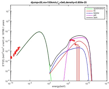
E*F(E) (keV

2/cm 2 s keV) at 19786.1 years

djump=20,vs=155km/s,f

b=3e6,density=5.850e-25

synchrotron IC bremz pi0 sum

Figure 3.20s=2.2

10-10 ₁₀-5 ₁₀0 ₁₀5 ₁₀10 ₁₀15

energy(keV)

10-6

10-5

10-4

10-3

10-2

10-1

100

101

E*F(E) (keV

2/cm 2 s keV) at 19786.1 years

djump=20,vs=155km/s,f

b=3e6,density=5.850e-25 synchrotron IC bremz pi0 sum

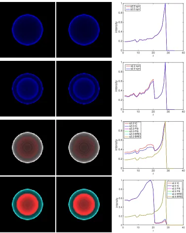
0 10 20 30 40 r 0 0.2 0.4 0.6 0.8 1 intensity s2.2 syn s2.0 syn

0 10 20 30 40

r 0 0.2 0.4 0.6 0.8 1 intensity s2.2 syn s2.0 syn

0 10 20 30 40

r 0 0.2 0.4 0.6 0.8 1 intensity s2.2 IC s2.0 IC s2.2 PI0 s2.0 PI0 s2.0 BREI s2.2 BREI

0 10 20 30 40

r 0 0.2 0.4 0.6 0.8 1 intensity s2.2 IC s2.0 IC s2.2 PI0 s2.0 PI0 s2.2 BREI s2.0 BREI

Figure 3.22First line: Synchrotron at 0.415×10−8_{keV. Second line: Synchrotron at 1.33 keV. Third}

line:Inverse Compton scattering (red), bremsstrahlung (green) andπ0_{-Decay (blue) at 1.33×10}6_{keV. Fourth}

line: Inverse Compton scattering (red), Bremsstrahlung (green) andπ0-Decay (blue) at 1.33×109keV s Left

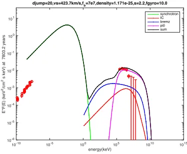
10-10 ₁₀-5 ₁₀0 ₁₀5 ₁₀10 ₁₀15

energy(keV)

10-6 10-5 10-4 10-3 10-2 10-1 100 101

E*F(E) (keV

2/cm 2 s keV) at 7803.2 years

djump=20,vs=423.7km/s,f

b=7e7,density=1.171e-25,s=2.2,fgyro=100.0

synchrotron IC bremz pi0 sum

Figure 3.23Gyrofactorη=100

10-10 ₁₀-5 ₁₀0 ₁₀5 ₁₀10 ₁₀15 energy(keV)

10-6

10-5

10-4

10-3

10-2

10-1

100

101

E*F(E) (keV

2/cm 2 s keV) at 7803.2 years

djump=20,vs=423.7km/s,f

b=7e7,density=1.171e-25,s=2.2,fgyro=10.0

synchrotron IC bremz pi0 sum

Table 3.3Parameter table for Fig. 3.11 to Fig. 3.26

figure number density jump fb us(k m/s) t(yr) s fgyro kei

Fig. 3.11 0.5845e-24 20 3e6 2 1 0.02

Fig. 3.12 0.5854e-24 uniform 3e6 2 1 0.02

Fig. 3.13 0.5854e-24 20 3e6 2 1 0.02

Fig. 3.14 0.1117e-24 20 1e7 424 7803.2 2.2 1 0.02

Fig. 3.15 0.1117e-24 20 3e6 424 7803.2 2.2 1 0.02

Fig. 3.17 0.1117e-24 20 1e7 424 7803.2 2.2 1 0.02

Fig. 3.18 0.5854e-24 50 1e7 352 9194.5 2.2 1 0.02

Fig. 3.20 0.5854e-24 20 3e6 155 19786.1 2.2 1 0.02

Fig. 3.21 0.5854e-24 20 3e6 155 19786.1 2.0 1 0.02

Fig. 3.23 0.1117e-24 20 7e7 424 7803.2 2.2 100 0.02

Fig. 3.24 0.1117e-24 20 7e7 424 7803.2 2.2 10 0.02

Fig. 3.26 0.1117e-24 28 7e7 341 9118.7 2.2 100 0.0005

Fig. 3.14 to Fig. 3.26 show radiation fluxes and corresponding images. Fig. 3.14 and Fig. 3.15 have different magnetic field strengths. In Fig. 3.14,Bis 6.67µG, and 2.0µG in Fig. 3.15. We can see that the magnetic field affects the synchrotron radiation significantly. Obviously, the one with a high value of synchrotron flux corresponds to the high value of magnetic field. Fig. 3.16 compares the intensity images at different energy for these two different situations. In all the images, Inverse Compton scattering is red, bremsstrahlung is green andπ0-decay is blue.

Fig. 3.17 and Fig. 3.18 are the cases with different outer densities. In Fig. 3.17, the outer density is 20 times higher than the inner density, and in Fig. 3.18 50 times higher. The different density structures have a great impact on all the radiation fluxes, with higher outer densities giving higher fluxes. Fig. 3.19 compares the images at different energy for these two different density structures. We observe a bump for both of the images at 1.33x109keV. The bump in the higher density jump is more obvious than the lower density jump one.

Fig. 3.20 and Fig. 3.21 illustrate different electron spectral index:s=2.2 in Fig. 3.20, ands=2.0 in Fig. 3.21. The shape of theπ0-decay spectrum is different, and all the fluxes in the case ofs=2.0 are higher. Since Fig. 3.22 shows that the image profiles are the same with different electron spectral index. Since both of them older compared with the previous cases, the synchrotron radiation profile has smaller circle in the larger one.

Fig. 3.23 and Fig. 3.24 have different gyrofactors:η=100 in Fig. 3.23 andη=10 in Fig. 3.24. The maximum energy is lower in Fig. 3.23. In Fig. 3.25, the majority of profiles are similar with different gyrofactorη. However, the peak of the IC is aroundr =20 forη=100, aroundr=17 forη=10 at 1.33x109keV.

0 10 20 30 40 r 0 0.2 0.4 0.6 0.8 1 intensity f100 syn f10 syn

0 10 20 30 40

r 0 0.2 0.4 0.6 0.8 1 intensity f100 syn f10 syn

0 10 20 30 40

r 0 0.2 0.4 0.6 0.8 1 intensity f100 IC f10 IC f100 PI0 f10 PI0 f100 BREI f10 BREI

0 10 20 30 40

r 0 0.2 0.4 0.6 0.8 1 intensity f100 IC f10 IC f100 PI0 f10 PI0 f100 BREI f10 BREI

Figure 3.25First line: Synchrotron at 0.415×10−8_{keV. Second line: Synchrotron at 1.33 keV. Third}

line:Inverse Compton scattering (red), Bremsstrahlung (green) andπ0_{-Decay (blue) at 1.33×10}6_{keV. Fourth}

line: Inverse Compton scattering (red), Bremsstrahlung (green) andπ0_{-Decay (blue) at 1.33×10}9_{keV. Left :}

10-10 10-5 100 105 1010 1015

energy(keV)

10-7

10-6

10-5

10-4

10-3

10-2

10-1

100

101

E*F(E) (keV

2/cm 2 s keV) at 9118.7 years

djump=28,vs=341km/s,f_b=7e7,density=1.171e-25,s=2.2,fgyro=100.0,kei=0.0005,zeta=1e-4

synchrotron IC bremz pi0 sum

Figure 3.26Example of a model providing a fairly good description of the Cygnus Loop (data points). Age 9118.7 years, current shock speed 341 km/s, cavity density 1.17 x 10−25_{g cm}−3_{, density jump a factor of}

28,fb=7 x 107, s=2.2, and gyrofactorη=100. This model explains the GeV emission as due toπ0decay,

in different colors are the result from my simulation. The model shows fairly good agreement and confirms the Cygnus Loop as a middle aged supernova remnant[Kat11]. The simulation of the energy range between 10−10_{to 10}−6_{keV agrees well with the observation. Both of the observation and the} simulation result have a highest flux point at a similar position. However, the simulation for the energy range between 106to 109keV decreases more slowly than the observational result.

3.3

Conclusion

We investigate the evolution of the dynamic information (speed, density, pressure profiles) of supernova remnants using the VH1 code. We compare our uniform model with the cavity model. The differences of synchrotron and bremsstrahlung andπ0-decay between the uniform model and the cavity model are small. However, IC depends on only one power of density, and we observe significant differences. The double shell structure happens in Fig. 3.8 and Fig. 3.9. For the total emission at 1 GeV and 1 TeV, in radial profiles. The centre emission of 1TeV is greater than at 1GeV. It shows the importance of hadronic and leptonic processes in cavity SNRs.

CHAPTER

4

INTRODUCTION TO GRANULAR FLOW

4.1

Granular media

We observe granular media everywhere in the world. There are different kinds of them, like sugar, sand or rice ... Fig. 4.1 provides some examples of granular media in the real world. Granular materials are the second most used material in industry[Dur12; Bat06]. Different kinds of industrial fields, including mining, foods, and pharmaceuticals, use granular media[And13]. The study of the fundamental theory of granular media helps people to build a deeper understanding of granular media’s behavior. It will be quite useful in fields like soil mechanics, fluid dynamics, or rheology, which can be applied in both industry and academia.

The task of studying granular flow raised several problems[And13; Cam90; Gol03; PR08; Rey85; Her13]. First, dealing with granular materials requires inspection of a large number of particles, and the interactions between particles are complex. Second, the methods used for gases or liquids, including Brownian motion or thermodynamics, doesn’t work for granular media directly. Third, there is no clear definition of the scale separation. Fourth, energy dissipation within granular materials must be accounted for.

information in Sec. 4.1.3).

Figure 4.1Different kinds of granular media[And13]

4.1.1 Granular packing

Different from liquids or gases, which are continuous, flows of dense granular media have their own properties. One property of granular media is its packing of grains. Scientists and engineers are interested in the study of packing of grains, like the optimization of grains’ storage. To describe the property of granular media, the variable volume fractionφis introduced. We use volume fractionφ to describe the ratio of the grains’ volume to the total volume:

φ≡Vgrains Vtotal