A Flexible Estimating Equations Approach for Mapping Function-Valued Traits

INVESTIGATION

A Flexible Estimating Equations Approach

for Mapping Function-Valued Traits

Hao Xiong,* Evan H. Goulding,†_{Elaine J. Carlson,}‡_{Laurence H. Tecott,}‡_{Charles E. McCulloch,*}

and S´aunak Sen*,1

*Department of Epidemiology and Biostatistics, University of California, San Francisco, California 94143,†_{Department of Psychiatry} and Behavioral Sciences, Northwestern University Feinberg School of Medicine, Chicago, Illinois 60611, and‡Department of Psychiatry, University of California, San Francisco, California 94143

ABSTRACTIn genetic studies, many interesting traits, including growth curves and skeletal shape, have temporal or spatial structure. They are better treated as curves or function-valued traits. Identification of genetic loci contributing to such traits is facilitated by specialized methods that explicitly address the function-valued nature of the data. Current methods for mapping function-valued traits are mostly likelihood-based, requiring specification of the distribution and error structure. However, such specification is difficult or impractical in many scenarios. We propose a general functional regression approach based on estimating equations that is robust to misspecification of the covariance structure. Estimation is based on a two-step least-squares algorithm, which is fast and applicable even when the number of time points exceeds the number of samples. It is also flexible due to a general linear functional model; changing the number of covariates does not necessitate a new set of formulas and programs. In addition, many meaningful extensions are straightforward. For example, we can accommodate incomplete genotype data, and the algorithm can be trivially parallelized. The framework is an attractive alternative to likelihood-based methods when the covariance structure of the data is not known. It provides a good compromise between model simplicity, statistical efficiency, and computational speed. We illustrate our method and its advantages using circadian mouse behavioral data.

M

ANY phenotypes (or traits) in genetic studies are quantitative and can be summarized by a single num-ber; examples include bone mineral density and body weight. Other traits of interest to geneticists such as growth curves (Krameret al.1998), circadian rhythms (Shimomura et al.2001), and morphology (Leamyet al.2008) have spatial or temporal structure and cannot be reduced to a single num-ber. Such traits may be viewed as curves or as function-valued (Pletcher and Geyer 1999). Quantitative genetics of such traits benefit from generalizations tailored to their function-valued nature (Kirkpatrick and Heckman 1989). In this arti-cle we present a new framework for identifying regions of the genome, quantitative trait loci (QTL) (Rapp 2000; Broman 2001), contributing to variation in function-valued traits.

Acknowledging the function-valued nature of a trait has several advantages. We can naturally treat features such as rates of growth or periodicfluctuations. We may also arrive at a more parsimonious representation of the data: a long sequence of correlated observations can often be described by a few values. From an evolutionary perspective, the function-valued nature of the data puts constraints on the patterns of variation possible and how selection might operate on the trait (Kingsolveret al.2001). For these rea-sons, application of functional data analysis (FDA) (Ramsay and Silverman 2005) to genetic data has been fruitful. Wu and Lin (2006) called genetic mapping of function-valued traits functional mapping. Function-valued traits have been variously referred to as infinite-dimensional traits, longitu-dinal traits, repeated measures, functional traits, and dy-namic traits (Kingsolveret al.2001).

Most existing methods for mapping function-valued traits use a likelihood framework where the analyst must specify the mean function, the error distribution, and the error structure. When those features can be specified, one can use parametric functional mapping (Ma et al. 2002; Wu et al.

Copyright © 2011 by the Genetics Society of America doi: 10.1534/genetics.111.129221

Manuscript received April 1, 2011; accepted for publication June 2, 2011

Supporting information is available online at http://www.genetics.org/content/ suppl/2011/06/24/genetics.111.129221.DC1.

2004; Wu and Lin 2006). Here the analyst specifies the form of the mean function (say logistic, for modeling growth curves) and the error function (say autoregressive Gaussian errors). If there is not enough information about the form of the mean function, one may model the mean function non-parametrically using different basis function families: Legen-dre polynomials (Lin and Wu 2006), orthogonal polynomials (Yang et al. 2006), B-splines (Yang et al. 2009; Yap et al. 2009), and wavelets (Zhao et al.2007) have all been used in the past. The approaches of Yanget al. (2009) and Yap et al.(2009) allow for an unstructured form of the variance– covariance matrix of the errors and use a multivariate Gauss-ian distribution. However, when the number of measure-ments per individual exceeds the number of samples and the empirical covariance matrix is thus singular, additional procedures such as wavelet dimension reduction (Zhao et al.2007) or regularized estimation of the covariance ma-trix must be employed. For likelihood-based methods, incom-plete genotype data are typically handled by the EM algorithm as in Lander and Botstein (1989). Bayesian formu-lations have been considered by Yang and Xu (2007) and Liu and Wu (2009).

In this report, we present an alternative framework for mapping function-valued traits on the basis of estimating equations. It is especially suited for scenarios where the error structure is unknown or poorly specified or when the number of time points exceeds the number of samples. Such data are becoming increasingly common with advances in automatic phenotyping. We present a mouse behavioral data set below that has these characteristics.

Our simulation studies indicate that likelihood functional regression models, when misspecified, may not have the desired false positive rates and can have lower power than our estimating equations approach. Generalized estimating equations have been used for mapping nonnormal traits (Lange and Whittaker 2001), but, to our knowledge, they have not been applied to mapping function-valued traits. Note that for genetic mapping, the covariance may be con-sidered a nuisance parameter; for evolutionary studies and animal breeding, the covariance function is a key para-meter of interest (Kingsolveret al.2001; Mezey and Houle 2005).

Central to our approach is a general linear functional model that can accommodate any number of covariates and use a single set of computer programs without modification for different numbers of covariates. We use a simple two-step least-squares estimation procedure that is comparable in speed and memory to regular linear regression. This fa-cilitates the use of commonly needed but computationally intensive procedures such as permutation tests for assess-ment of critical values or multiple testing correction, multiple imputation of incomplete genotypes, and model selection procedures.

Our article is organized as follows. The Mouse Behav-ioral Datasection describes a mouse behavior data set that motivated our method. Then in Model and Estimation

we outline the statistical theory underlying our method, in-cluding the model, estimation, and testing methods. We examine the method’s characteristics in simulations and on the mouse behavioral data in Simulation Studies and Data Analysis. We conclude with a summary in the Discussion.

Mouse Behavioral Data

(polymorphic) autosomal markers between these two strains. The average marker distance was 9.7 Mb (median 8.0 Mb, range 0.2–35 Mb). For phenotyping, mice were individually housed for 16 days in a home cage monitoring system that is described in detail elsewhere (Goulding et al. 2008). Briefly, this system allowed automated collection of feeding (detection of photobeam breaks when mice access food), drinking (detection of capacitance change with lick contacts at water spout), and movement (load cell position plat-form) data under a 12:12 light:dark cycle (lights on at 7AMand off at 7PM).

Data were processed for errors in detection of feeding, drinking, and movement events as previously described (Goulding et al. 2008). Only mice with at least 4 days of complete data were used for subsequent analysis. Mice were allowed 4 days of acclimation to the monitoring cages and thefinal 12 days of data were used for analysis.

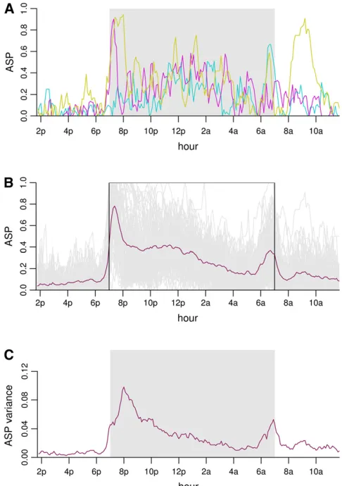
Mice in their home cages exhibit transitions between two major distinct states: an active state where the animals en-gage in bouts of feeding, drinking, and locomotion and an inactive state in which the animals engage in prolonged episodes of minimal movement at a discrete home base location (Gouldinget al. 2008). Transitions between active and inactive states were identified with a resolution of 20 msec; the data then were aggregated into 6-min bins across all analysis days. Thus, each measurement represents the probability that an individual mouse was in the active state (active state probability, ASP) during any 6-min interval across all analysis days (Goulding et al.2008).

As indicated earlier, the data showed several features that motivated the development of new methodology:

1. The number of measurements per mouse (220) exceeds the number of mice (89), which presents problems for

many methods as the empirical covariance matrix is singular.

2. There is considerable variation in individual mouse active state probabilities (Figure 1, A and B).

3. The distribution is awkward to describe. There are mice with active state probabilities of zero or one at some time points.

4. The variance between individuals as a function of time is smooth with two peaks (Figure 1C).

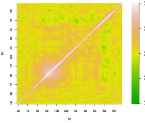
5. The average ASP pattern is also smooth with two peaks: one at 7–9PMand one at 6–8AM. There is a third mod-erate peak between these two peaks. There is a minimum or nadir at night at 4–6 AM. Note, however, that usual transformations of the data (such as the arcsine transforma-tion) failed to stabilize the variance (results not shown). 6. The correlation between time points was also smooth but

without an easily articulated structure (Figure 2).

Model and Estimation

We outline our method in this section. We start with the functional regression model. Using estimating equations, the parameter estimates and test statistics have a closed-form so-lution, assuming complete genotype data. Next, we present some extensions that broaden the method’s applicability and de-scribe our strategy for handling incomplete genotypes. Finally, we discuss the computational requirements of our method, ba-sis function choice, and shrinkage estimation of the covariance.

Model

a linear regression model is traditionally used for mapping a quantitative trait,

y¼z1b1þz2b2þ⋯þzpbpþe;

where y is the quantitative trait of interest, and zk, k = 1,. . .,p, are covariates,bk, k= 1,. . .,p, are the effects of the covariates, andeis the random error. The covariates may include an intercept, the QTL genotypes, and any other fac-tors such as age, sex, or body weight that may contribute to the trait. The focus of QTL mapping is to identify the genetic covariates contributing to the trait.

Analogously, we use a functional regression model for our function-valued trait when complete genotype data are available. Lety(t) be the function describing the observable trait as a function oft; in the remainder of our treatment we consider t to be time, but it can be extended to consider spatial position in one or more dimensions. We assume that the function can be represented as follows in terms of cova-riatesz1,z2,. . .,zp(that may include genotypes),

yðtÞ ¼z1b1ðtÞ þz2b2ðtÞ þ. . .þzpbpðtÞ þeðtÞ

¼X

p

k¼1

zkbkðtÞ þeðtÞ; (1)

wherebk(t),k= 1,. . .,p, are unknown functions, ande(t) is random error. We assume that each of the bk(t) functions can be represented as afinite linear combination of a family

of basis functions (say splines, polynomials, or Fourier se-ries) as

bkðtÞ ¼bk1c1ðtÞ þbk2c2ðtÞ þ. . . þbkqcqðtÞ ¼ Xq

l¼1

bklclðtÞ;

where qis the number of basis functions. The number and nature of the covariates z1, z2,. . .,zp will depend on intended use. They may include a single QTL, multiple QTL with or without interaction effects, or nongenetic cova-riates such as age and sex.

Suppose there are nindividuals with yi(t) denoting the function-valued trait for theith individual. Further suppose that the trait is observed at m times, t1, t2,. . .,tm. If we denote byyijthe trait value for theith individual attj, then we can represent the observed trait data as ann·mmatrix,

Y¼ ½yijn·m:

Let zik denote the value of the kth covariate in theith individual,cjl=cl(tj) be the value of thelth basis function at thejth time pointtj, and leteijbe the random error for the ith individual at thejth time point. In matrix notation, we write

Z¼ ½zikn·p; C¼ ½cjlm·q B¼ ½bklp·q; andE¼ ½eijn·m:

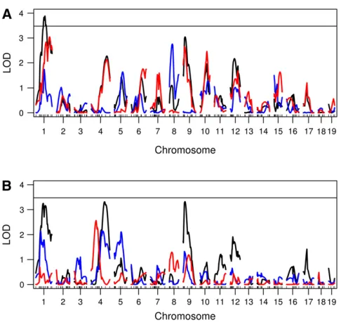
Then, it can be shown that Figure 3 Genome scans using a nonfunctional approach. (A) Genome

scans for total daily ASP (black), dark cycle onset peak (blue), and mid-dark cycle (red). (B) Genome scans for mid-dark cycle nadir (black), mid-dark cycle offset peak (blue), and light cycle activity (red). The solid horizontal lines are the 5% permutation threshold for the maximum of the six genome scans, which adjusts for the fact that we are examining six correlated genome scans.

Y¼ZBCTþE: (2)

Writingy= vec(YT_{),e= vec(E}T_{),b= vec(B}T_{), andX=} Z5C, where5denotes the Kronecker product and vec is an operator that stacks columns of a matrix into a single, large column vector, the above equation can be written in the familiar form

y¼Xbþe:

If thenindividuals are independent with common covari-ance matrix, thenL= var(e) = var(vec(E)) =In5S, where S is the covariance matrix of (e(t1),e(t2),. . .,e(tm))T. Note thatS is, in general, unknown and must be estimated from the data.

Estimation

As stated earlier, without a distributional assumption for the random error, we cannot write out a likelihood function. Instead we choose B (or equivalently b) to minimize the residual sum of squares,

SðbÞ ¼ ðy2^yÞTðy2^yÞ ¼vecðY2Y^ÞvecðY2Y^ÞT; (3)

where^y¼vecðY^TÞis an estimate depending onb^¼vecð^BTÞ. The criterion, Equation 3, is an approximation to the inte-grated squared error of the estimate

ðt*

t*

ðyðtÞ2^yðtÞÞ2dt;

where [t*,t*] is the range of the interval we wish to con-sider. Assuming that the range of observed time points is close (or identical) to the range we wish to consider, the integrated squared error may be approximated by the sum

Xm

j¼1

yðtjÞ2^yðtjÞ 2

:

Optimizing this criterion is equivalent to solving a least-squares problem that has a closed-form solution,

^

BT¼ ðCTCÞ21CTYTZðZTZÞ21: (4)

This can be seen as a combination of two least squares: one on basis functions (theCpart) and the other on geno-types (theZpart). The least-squares equations are thus our estimating equations; the resulting solution is asymptotically unbiased (Liang and Zeger 1986). Further, a consistent es-timate of the variance of the eses-timated coefficients is obtain-able if a consistent estimate of the residual covariance matrix, S, is available. Note that estimation of the coeffi -cients does not require knowledge or estimation ofS.

The variance of the estimate is

var

^

b¼ ðZTZÞ215

ðCT_CÞ21_CT_SCðCT_CÞ21_[t: (5)

The predictions are

^

Y¼

ZðZTZÞ21ZTÞYðCðCTCÞ21CT

:

In the context of statistical methods for longitudinal data, our approach corresponds to using estimating equations with a working independent correlation structure and assuming a Gaussian distribution. In general, these esti-mates will be less efficient compared to a correctly specified likelihood model (Godambe 1960). However, significant loss of efficiency seems to be the exception rather than the rule (Diggle et al. 2002; Chandler and Bate 2007; McCulloch et al.2008). We explored this in our simulations (see Sim-ulation Studies and Data Analysis).

Testing

LOD score. Instead, we consider two related quantities as explained below. These can be used as test statistics to test the null hypothesis at each locus; i.e., genetic variation at that locus does not contribute to (function-valued) trait variation.

Consider the trait model in Equation 1. The standard null hypothesis is no effect; that is, some bk(t) are identically zero, which is same as the coefficients of their basis expan-sion being zero. Suppose the null hypothesis isB= 0 (testing select entries by replacingBwithSBin Equation 4, whereS is a selection matrix so thatSBselects specific columns ofB, and subsequent derivations would be based on modified estimation).

Wald statistic:Let vec

ð

^BT

Þ

be the estimate of coefficients in vector form and ^t be the estimated covariance matrix of vec

ð

^BT

Þ

. The quadratic form

vec

ð

^BT

Þ

T^t21vec

ð

B^T

Þ

(6)

follows a Hotelling’s T2 _{statistic with parameters d and r,} wheredis the degrees of freedom of the estimate oft (Equa-tion 5) andris the length of vec(BT_{). For reasonably large} sample sizes, this can be approximated by ax2_{-statistic with} rd.f.

The estimate of the covariance matrixtis

^

t¼ ðZTZÞ215

ðCT_CÞ21_CT_SC^ _ðCT_CÞ21_;

whereS^ is an estimate ofS. The simplest estimate one can consider is formed from the residuals:

^

S¼ 1 n2p

Xn

i¼1

yi2^yi

yi2^yi T

:

This estimate is unbiased, but one may also want to consider biased estimates as discussed later in this section.

Residual error statistic: An alternative statistic would be the difference in residual sum of squares between the model with the genetic locus and a null model corresponding to the null hypothesis. Thus, if Y^0 denotes the fitted values from the null model, and Y^1 denotes thefitted values from the model including the genetic locus under consideration, we would calculate Si¼vecðY2Y^iÞTvecðY2Y^iÞ; i¼0; 1 and then use

S02S1 S1

as a test statistic. This statistic is closely connected to the proportion of the variance explained by the locus. The asymptotic null distribution of this statistic is a mixture of x2_{-variables (Rotnitzky and Jewell 1990; Shen and Faraway} 2004). The mixing proportions depend on the eigenvalues of a matrix depending onCandS.

Assessing significance: As stated earlier, the Wald statistic has an asymptotic x2_{-distribution, while the distribution of} the residual error statistic is more complicated. The genome-wide significance of either can be established by a permu-tation test (Churchill and Doerge 1994). For genome-wide association studies (GWAS), one may contemplate a Bonfer-roni correction or a false discovery rate correction on point-wise P-values. In this context the Wald statistic would be more convenient.

Incomplete genotypes

The functional regression model (Equation 1) assumed that we have complete genotypes;i.e., the genotype of every in-dividual at every genomic location is known. In practice this is rarely the case, as there are gaps between typed markers, genotyping reactions for some individuals may fail, or selec-tive genotyping may have been used. A key part of the QTL mapping problem is to accommodate incomplete genotype data. If typed markers are reasonably dense and no selective genotyping is used, one can use Haley–Knott regression (Haley and Knott 1992). Here we replace the indicator var-iables corresponding to possible genotypes at a locus by their probabilities conditional on typed markers. Then we use functional regression as if we had complete genotypes. This method is very fast, and easily parallelized, but is sus-ceptible to bias when selective genotyping is used or when the marker spacing is big (Kao 2000; Senet al.2005). In such cases we can use multiple imputation (Sen and Churchill 2001). For both multiple imputation and Haley–Knott re-gression the analyst can contemplate different functional regression models for the trait without needing any addi-tional computaaddi-tional machinery.

Computational considerations

The modularity of our algorithm also simplifies computa-tion. If we assumenandmare greater thanpandq, then a naive application of least squares to they=Xb+e prob-lem, whereXmn·pq, would be in the order ofO(p2_q2_nm + p3_q3_{) (Golub and Van Loan 1996). In our method, we} solve two smaller least-squares problems. In Equation 4, the two inverses are of orderO(mq2_+q3_+np2_+p3_{), while} other matrix multiplications add O(mnq+npq).

Furthermore, only the part involvingZneeds to be recom-puted for different loci, while the rest can be comrecom-puted once and saved for later use. Likelihood-based methods employing the EM algorithm cannot take advantage of this; every in-stance of the EM algorithm has to be run separately. Suppose we are performingrpermutations, and usingsimputations, the complexity will beO(mq2_+q3_+mnq+lrs(np2_+p3₊ npq)) forlloci. Use of the EM algorithm for maximum likeli-hood also has the disadvantage that it requires modification each time the function regression model is changed.

Basis functions

important in functional regression and an active research area. As this is beyond the scope of this article, we note only that the family and number of basis functions are key choices and can beflexibly accommodated with our method. We used B-splines for the mouse behavior data and natural splines for the simulations.

Shrinkage estimation ofS

When the number of individuals is greater than the number of time points, the obvious estimate of S is the empirical covariance of residuals. It is unbiased, but may suffer from high variance (Kauermann and Carroll 2001). If the number of time points (m) is large relative to the number of individ-uals (n), the analyst may consider using a biased estimator such as the shrinkage estimator proposed by Ledoit and Wolf (2004) and adapted by Schafer and Strimmer (2005). The resulting covariance estimate is nonsingular (unlike the em-pirical estimate when the number of individuals is smaller than the number of time points). We evaluate this choice in a simulation study in the next section. Shrinkage estimation of the genetic covariance for function-valued data has been considered by Meyer and Kirkpatrick (2010).

Additional practical considerations

In our development we assumed that there were no missing trait data. If there is a modest amount of missing trait data, we can use local smoothing methods such as smoothing splines to fill in the missing data. Alternatively, one can incorporate estimation of missing data into the estimation procedure by using a basis expansion on the left-hand side of Equation 2 and replacingYwith the coefficients of the expansion.

Our estimating equations correspond to assuming homo-scedasticity and independence between time points. We can easily accommodate heteroscedasticity by using weighted least squares instead of ordinary least squares. There can be weights on individuals and/or different time points. More generally, if the analyst has prior knowledge about the covariance between samples or time points, it can be used to increase efficiency, yet the method will remain robust to their misspecification.

Simulation Studies and Data Analysis

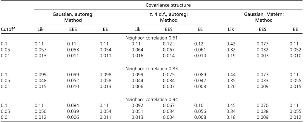
We conducted three simulation studies and analyzed the mouse behavioral data presented earlier, to evaluate our method. We studied its type-I error and power and compared it to other methods (functional and nonfunc-tional). In the first simulation study, we compared our method to a parametric likelihood-based functional map-ping method based on Ma et al.(2002). We computed the type-I error under three covariance structures. In the second simulation study we compared our method to a likelihood-based method that estimates the covariance (Yap et al. 2009). In addition, we looked at the power of different methods. In the third simulation study, we compared our method with a nonfunctional method (a cross-sectional method), which compresses multiple observations within a sample into a summary statistic by averaging; this material is inSupporting Information,File S1 Figure S1, and Table S1 Finally, we applied both the Wald statistic and the in-tegrated residual error statistic to our mouse behavioral data and compared the result to a cross-sectional method (taking Table 1 Null distribution P-values from parametric and estimating equation approaches under three error distributions using 1000 simulations each

Covariance structure

Gaussian, autoreg: Method

t, 4 d.f., autoreg: Method

Gaussian, Matérn: Method

Cutoff Lik EES EE Lik EES EE Lik EES EE

Neighbor correlation 0.61

0.1 0.11 0.11 0.11 0.11 0.12 0.12 0.42 0.077 0.11

0.05 0.057 0.053 0.054 0.064 0.067 0.061 0.32 0.032 0.052

0.01 0.013 0.011 0.011 0.016 0.014 0.010 0.19 0.007 0.010

Neighbor correlation 0.83

0.1 0.099 0.099 0.098 0.099 0.075 0.089 0.44 0.077 0.11

0.05 0.048 0.052 0.058 0.044 0.034 0.042 0.35 0.033 0.055

0.01 0.015 0.010 0.013 0.006 0.007 0.008 0.20 0.009 0.015

Neighbor correlation 0.94

0.1 0.11 0.084 0.11 0.092 0.067 0.10 0.45 0.070 0.11

0.05 0.050 0.039 0.054 0.051 0.034 0.056 0.34 0.038 0.055

0.01 0.012 0.006 0.011 0.013 0.004 0.008 0.18 0.009 0.012

means over time intervals) that is currently used to analyze such data (Nishiet al.2010).

Simulation studies: Comparison with a parametric functional approach

Here we report simulation studies comparing our estimating equations approach to a likelihood-based parametric ap-proach. Our objective was to compare the null distribution and power of our method against likelihood-based func-tional mapping under three conditions: when the likelihood model is correctly specified, the pointwise error distribution is incorrectly specified, and the covariance is misspecified.

Our simulations were loosely modeled after the poplar tree data in Ma et al.(2002). We assumed that 13 equally spaced measurements between times 0 and 6 were made on 200 individuals; 100 individuals each had one of two possi-ble genotypes 0 and 1. The mean of the observations was assumed to follow a logistic curve as in Maet al.(2002) with the functional form

yðtÞ ¼ u0

1þu1expð2u2tÞþeð

tÞ; (7)

whereu= (u0,u1,u2) are parameters describing the mean curve, ande(t) is a stationary stochastic process with mean 0 and point-wise variances2_{= 0.01. The functional} param-eters of individuals with genotypes equal toiare described byui_{,i= 0, 1. Under thealternative,u}0_{= (1.00, 9.0, 1), and} u1_{= (0.95, 8.5, 1). Under thenull,u}0_=u1_{= (0.975, 8.75,} 1). The plots of three mean functions are inFigure S2.

We considered three error structures:

Gaussian, autoregressive: The marginal (pointwise) and all finite-dimensional distributions of the error are Gaussian, and the correlation structure is autoregressive so that the covariance between measurements separated by a timetis described by the exponential correlation functionr(t) = s2_rt_{. We evaluated performance under r = 0.61, 0.83,} 0.94, which are the correlations between successive time points for the Matérn correlation function (with

smooth-ness parameters 0.5, 1, and 2, respectively) considered below (see File S1for definition of the covariance func-tion and references).

t-distributed, autoregressive: The finite-dimensional distri-butions have a t-distribution with 4 d.f. (the smallest for which the third moment exists). The correlation func-tion is autoregressive, as above.

Gaussian, Matérn: The finite-dimensional distributions are Gaussian, and the correlation function is Matérn with amplitude parameters2_{, scale parameter 1, and} smooth-ness parameters 0.5, 1, and 2. The three correlation func-tions are shown inFigure S3.

We compared three functional approaches:

Likelihood (Lik): We used the likelihood-based method pre-sented in Maet al.(2002). This assumes that the mean function has a logistic form and that the errors are Gauss-ian with an autoregressive structure.

Estimating equations (EE): We used the Wald statistic with-out a shrinkage estimator for the error covariance matrix, S. The mean function was modeled using a natural spline basis with 7 d.f.

Estimating equations with shrinkage (EES): We used the Wald statistic with a natural spline basis with the Schafer and Strimmer (2005) method for shrinking the covari-ance matrix.

Note that the estimating equations approach is applied using no knowledge of the mean and correlation functions. The likelihood method is correctly specified for the first set of simulations (Gaussian, autoregressive). It misspeci-fies the finite-dimensional distributions in the second set (t-distributed, autoregressive), but the correlation is cor-rectly specified. In the third set, the correlation functions are misspecified.

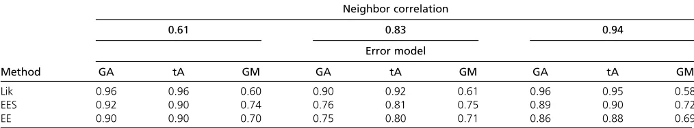
Table 1 gives tail probabilities of the test statistics under the null. It shows that the correctly specified likelihood-ratio statistic hasx2_{-tail probabilities as expected. This holds} true when the marginal distribution of the errors has a t-distribution as well. However, when the correlation structure Table 2 Power of parametric and estimating equations approaches under three error distributions: Gaussian, autoregressive (GA);t, 4 d.f., autoregressive (tA); and Gaussian, Matérn (GM)

Neighbor correlation

0.61 0.83 0.94

Error model

Method GA tA GM GA tA GM GA tA GM

Lik 0.96 0.96 0.60 0.90 0.92 0.61 0.96 0.95 0.58

EES 0.92 0.90 0.74 0.76 0.81 0.75 0.89 0.90 0.72

EE 0.90 0.90 0.70 0.75 0.80 0.71 0.86 0.88 0.69

is misspecified, it no longer has ax2_{-distribution and the type-I} errors corresponding to all the critical values are higher than expected.

The simulations indicate that the regular estimating equations approach has near the expected type-I error behavior under all circumstances. However, the estimating equations approach with shrinkage does not have this property with slightly too low type-I error rates, and thus its null distribution would need to be obtained empirically using permutations. The likelihood-ratio statistic has the expectedx2_{-distribution only when the correlation structure} is correctly specified; otherwise it may be way off target. Thus, in practice, if the covariance is hard to specify, the likelihood-ratio statistic’s statistical significance should be established using a permutation distribution.

Since the null distribution of the statistics is not always as expected, we used the null distribution quantiles as the critical values to calculate power (Table 2). Wefind that the likelihood approach has the greatest power when the corre-lation structure is correctly specified (note that the likeli-hood method in this case also benefits from having the correct mean function). The estimating equations ap-proaches have greater power when the correlation structure is incorrectly specified. In all situations, the estimating equa-tions with shrinkage has slightly greater power than the approach without shrinkage. Thus, our simulations demon-strate that power of likelihood methods may be compro-mised if the correlation structure is misspecified (even if the type-I error has been recalibrated).

Simulation studies: Comparison with parametric functional method with unstructured covariance

Yap et al. (2009) proposed using regularized covariance estimation within the framework of parametric likelihood-based functional mapping. The regularization parameter was selected by 10-fold cross-validation and assumed con-stant throughout a marker interval.

We performed simulations using the same scenario as in Yap et al. (2009). We simulated a 100-cM linkage group

with six equally spaced markers with a QTL at 32 cM. The associated phenotypes were sampled from a multivariate Gaussian distribution with logistic function describing the mean function conditional on the QTL genotypes. There are three genotypes with three mean curves following logis-tic functions as in Equation 7: thefirst genotype hasu0= 30, u1= 5,u2= 0.5; the second genotype hasu0= 28.5,u1= 5, u2= 0.5; and the third genotype hasu0= 27.5,u1= 5,u2= 0.5. Each individual is observed at 10 time points. The re-sidual error was assumed to be multivariate normal, with three different covariance structures:

1. S1is autoregressive withs2= 3,r= 0.6. 2. S2is equicorrelated withs2= 3,r= 0.5.

3. S3is an“unstructured”covariance matrix, as given in Yap et al.(2009) (reproduced inFile S1). It does not have an easily described structure.

All parameter values including the covariance matrices are taken from Yap et al. (2009). We ran 10,000 simulation replicates to obtain stable estimates; Yapet al.(2009) had 100 simulation replicates.

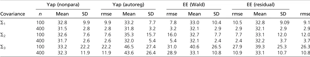
The LOD score (or linkage test statistic) was calculated every 4 cM, resulting in 26 loci. As in the simulations reported by Yapet al.(2009), for each simulation, we esti-mated the location of the QTL as the location of the maxi-mum LOD score. The average, standard deviation, and root mean squared error of QTL location estimates were com-pared. Lower root mean squared error indicates a better method. (Note that we are unable to compare the power of the methods as we do not have access to the software used in the Yapet al.2009 article and are restricted to what was reported in the article.) The results are in Table 3.

We found that our method performed comparably to Yap et al.’s (2009) method for the most part, except forS3with a small sample size of 100, where Yapet al.’s (2009) method had better mean and slightly smaller standard deviation. But looking at the large values of standard deviations for all methods, it is clear that no method performed satisfactorily with this small sample size. ForS3with sample size 400, the Table 3 Mean, standard deviation, and root mean squared error of the genome scan peak in simulations using our method and that of Yapet al.(2009)

Yap (nonpara) Yap (autoreg) EE (Wald) EE (residual)

Covariance n Mean SD rmse Mean SD rmse Mean SD rmse Mean SD rmse

S1 100 32.8 9.9 9.9 33.2 7.7 7.8 33.0 10.4 10.5 32.8 9.09 9.1

400 31.5 2.8 2.8 31.8 3.2 3.2 32.1 2.9 2.9 32.1 2.9 2.9

S2 100 32.6 7.6 7.6 35.3 15.7 16.0 32.7 7.7 7.7 33.1 12.0 12.0

400 31.7 2.6 2.6 32.0 5.4 5.4 32.1 2.4 2.4 32.2 3.7 3.7

S3 100 33.2 22.2 22.2 46.5 27.4 31.0 40.6 26.5 27.9 39.3 25.3 26.3

400 32.3 11.9 11.9 43.6 26.4 28.9 33.1 10.8 10.9 33.1 10.7 10.8

The true QTL is at 32 cM. The columns labeled“Yap (nonpara)”and“Yap (autoreg)”are derived from Tables 1 and 2 of Yapet al.(2009). They refer to the results of using the likeihood-based methods of Yapet al.(2009) with an estimated regularized covariance and autocorrelated covariance, respectively. The columns labeled“EE (Wald)”and

performance of both methods was again comparable. Note, however, that our method is considerably simpler to imple-ment and has lower computational complexity.

Data analysis

Please refer to the Mouse Behavioral Data section for the details of the mapping population, markers, and phenotypic data collection. Our analytic goal was to detect genetic loci that contribute to individual variation in the shape of the curve describing how ASP changes with time of day. We applied our method using the Wald statistic and the residual error statistic. We also applied a nonfunctional approach informed by prior knowledge and a visual exploration of the data. The approach tries to mimic what we might do if we did not have a functional method at our disposal. It par-allels the approach taken recently by Nishiet al. (2010) for similar homecage movement data in consomic strains. Note that a credible parametric model for mouse behavior cannot be easily specified, and thus we cannot use a parametric func-tional method.

Nonfunctional method

We constructed six measures on the basis of the marginal distribution of the ASP curves as shown in Figure 1. Note that the change in active state probability with time of day exhibited by the mice appears to be divided intofive phases. During the dark cycle, there is an onset peak (7–9 PM) in active state probability that then decreases somewhat, exhibiting a broad peak from 9PM to 4AMfollowed by a dark cycle nadir from 4 to 6AM. An offset peak (6–8AM) in the active state probability then occurs near the end of the dark cycle. Finally, the active state probability is low throughout the majority of the light cycle. On the basis of these obser-vations we segmented the day into the following phases to measure the probability that a mouse was in the active state:

1. Daily: This is the mean over all time points.

2. Dark cycle onset peak: This is the mean over 7–9PM. 3. Mid-dark cycle: This is the mean over 9PM–4AM. 4. Dark cycle nadir: This is the mean over 4–6AM. 5. Dark cycle offset peak: This is the mean over 6–8AM. 6. Light cycle: This is the mean over 8 AM-12 noon and

2–7PM.

We performed genome scans using the Haley–Knott method (Haley and Knott 1992) for each of these measures. To correct for the fact that we used six correlated genome scans, we calculated a genome-wide threshold for the max-imum of the six genome scans, using 1000 permutations. Using the 5% multiple-scan corrected threshold we found only one locus on chromosome 1 for daily ASP (Figure 3).

Functional method

We used B-splines as our basis functions. We applied 10-fold cross-validation to the behavioral data, ignoring the geno-type data, to select the number of basis functions to use for

smoothing. We selected the smallest number of basis functions that gave a residual sum of squares within one standard deviation of the least value. This led us to select B-splines with 16 d.f. with equally spaced knots. These basis functions were used for all genome scans.

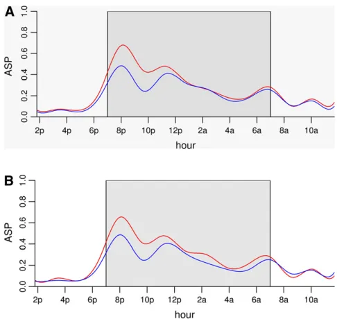
We performed genome scans using the Haley–Knott method with both the Wald statistic and the residual error statistics. We used 1000 permutations to establish genome-wide statistical significance. Using the functional approach and the 5% genome-wide threshold, we found two loci (on chromosomes 1 and 9) using the residual error statistic (Fig-ure 4A) and one locus on chromosome 9 using the Wald statistic (Figure 4B). The estimated genetic effects of the two loci are shown in Figure 5. Thus, in this example, the Wald statistic appears to be less sensitive than the residual error statistic.

Discussion

We have presented a new approach based on estimating equations for mapping function-valued traits. It is an at-tractive alternative to likelihood-based methods, especially when we have incomplete knowledge of the covariance structure or when the number of time points exceeds the number of samples. While information about the covariance can be incorporated to improve efficiency, our method is robust to its misspecification. Relative to a correctly spec-ified likelihood model, the estimating equations approach may be slightly less efficient. However, such loss was modest in our simulations and other studies (Chandler and Bate 2007). We thus believe that our method would be a good choice in most settings where the analyst is un-certain about the error distribution. The mouse behavioral data we presented are such an example. Likelihood meth-ods may be preferred, say, for traits such as growth curves, which have a long history of study, lending confidence to the data model.

Misplaced confidence in the covariance structure may have a price, as our simulations indicate. Likelihood-based methods with a misspecified covariance may not have the target type-I error and may have lower power than the estimation equations method. Although the anticonservative behavior of a misspecified likelihood observed in our sim-ulations may be rectified by a permutation test, that has an additional computational cost. This cost is manageable for QTL mapping in experimental crosses, but less so in GWAS where a correctly calibratedP-value is desired at each locus. Thus, the estimating equations Wald statistic has an edge in GWAS.

wavelets for dimension reduction as a separate step, we per-form dimension reduction and functional mapping in one step. Computational efficiency, as opposed to statistical effi -ciency, plays a bigger role for high-dimensional data. If the number of time points is very large or if model selection, permutation testing, or multiple imputation is needed, computational time increases severalfold. In such settings, our method has a clear advantage, as it is based on two low-dimensional least-squares operations: it can be computed quickly and does not involve any complex optimization cedures. The computational advantage is particularly pro-nounced when covariance structure defies easy specification. While Yap et al.’s (2009) method does not rely on specifi -cation of covariance structure, it comes at the expense of a generalized EM algorithm that must numerically solve a nonlinear optimization problem as part of the M-step. For large-scale studies with dense genotyping, computational efficiency is essential.

The estimating equation approach for mapping function-valued traits can be adapted for different situations. Our formulation assumes that the error variance is independent of the mean, which might not hold for traits whose point-wise marginal distribution is markedly non-Gaussian such as Poisson-distributed count data. A simple change to the sandwich estimator in Equation 5 can be used to obtain a robust variance estimate in this scenario. This involves replacing the estimate by a sum ofn terms with the same form as in Equation 5, with S replaced by the empirical multivariate residual for each individual. Another extension is when trait data on all individuals are not observed on the same set of time points. While small amounts of missing trait data can be dealt with by smoothing or imputation, the more general problem of uneven time points is more chal-lenging. The approach of Yaoet al.(2005) may offer a res-olution under Gaussian modeling assumptions.

In summary, our estimating equation method based on a general functional linear model makes few distributional assumptions. It has broad applicability to genetic studies and has opened an attractive alternative avenue to functional mapping distinct from likelihood methods. The possible improvements and adaptations listed above suggest the method’s promise andflexibility. Data and software used in this paper are available inFile S2. The mouse behavior data also is available at http://www.qtlarchive.org; updated ver-sions of the software will be posted at http://www.biostat. ucsf.edu/sen/software/.

Acknowledgments

Genotyping was carried out in the DNA Technologies Core at the University of California, Davis, Genome Center. We thank Ethelyn Layco for animal care, sample preparation for Illumina genotyping, and assistance with behavioral experi-ments. We thank Rongling Wu for providing Matlab code for the likelihood method that we adapted for use in R, Karl Broman and Tom Juenger for helpful comments, and Sandra

Erickson for suggesting we work on mapping function-valued traits. Some computations were performed using the University of California, San Francisco, Biostatistics High Performance Computing System. This research was sup-ported by grants from the National Institutes of Health (GM078338, GM074244, and DK072187).

Literature Cited

Broman, K. W., 2001 Review of statistical methods for QTL map-ping in experimental crosses. Lab Anim. (NY) 30(7): 44_–52. Chandler, R. E., and S. Bate, 2007 Inference for clustered data

using the independence loglikelihood. Biometrika 94(1): 167_– 183.

Churchill, G. A., and R. W. Doerge, 1994 Empirical threshold values for quantitative trait mapping. Genetics 138: 963–971. Diggle, P., K. Liang, P. Heagerty, and S. Zeger, 2002 Analysis of

Longitudinal Data, Ed. 2. Oxford University Press, London/New York/Oxford.

Godambe, V., 1960 An optimum property of regular maximum likelihood estimation. Ann. Math. Stat. 31: 1208–1211. Golub, G., and C. Van Loan, 1996 Matrix Computations. Johns

Hopkins University Press, Baltimore.

Goulding, E., A. Schenk, P. Juneja, A. MacKay, J. Wade et al., 2008 A robust automated system elucidates mouse home cage behavioral structure. Proc. Natl. Acad. Sci. USA 105(52): 20575_–20582.

Haley, C., and S. Knott, 1992 A simple regression method for mapping quantitative trait loci in line crosses using _flanking markers. Heredity 69: 315_–324.

Kao, C. H., 2000 On the difference between maximum likelihood and regression interval mapping in the analysis of quantitative trait loci. Genetics 156: 855–865.

Kauermann, G., and R. Carroll, 2001 A note on the efficiency of sandwich covariance matrix estimation. J. Am. Stat. Assoc. 96 (456): 1387–1396.

Kingsolver, J., R. Gomulkiewicz, and P. Carter, 2001 Variation, selection and evolution of function-valued traits. Genetica 112: 87–104.

Kirkpatrick, M., and N. Heckman, 1989 A quantitative genetic model for growth, shape, reaction norms, and other infi nite-dimensional characters. J. Math. Biol. 27(4): 429–450. Kramer, M., T. Vaughn, L. Pletscher, K. King-Ellison, E. Adamset al.,

1998 Genetic variation in body weight gain and composition in the intercross of Large (LG/J) and Small (SM/J) inbred strains of mice. Genet. Mol. Biol. 21(2): 211_–218.

Lander, E. S., and D. Botstein, 1989 Mapping Mendelian factors underlying quantitative traits using RFLP linkage maps. Genet-ics 121: 185_–199.

Lange, C., and J. Whittaker, 2001 Mapping quantitative trait loci using generalized estimating equations. Genetics 159: 1325. Leamy, L. J., C. P. Klingenberg, E. Sherratt, J. B. Wolf, and J. M.

Cheverud, 2008 A search for quantitative trait loci exhibiting imprinting effects on mouse mandible size and shape. Heredity 101(6): 518–526.

Ledoit, O., and M. Wolf, 2004 A well-conditioned estimator for large-dimensional covariance matrices. J. Multivariate Anal. 88 (2): 365–411.

Liang, K., and S. Zeger, 1986 Longitudinal data analysis using generalized linear models. Biometrika 73: 13–22.

Lin, M., and R. Wu, 2006 A joint model for nonparametric func-tional mapping of longitudinal trajectory and time-to-event. BMC Bioinformatics 7(1): 138.

Ma, C., G. Casella, and R. Wu, 2002 Functional mapping of quan-titative trait loci underlying the character process: a theoretical framework. Genetics 161: 1751.

McCulloch, C. E., S. R. Searle, and J. M. Neuhaus, 2008 Generalized,

Linear,and Mixed Models, Ed. 2. Wiley, New York.

Meyer, K., and M. Kirkpatrick, 2010 Better estimates of genetic covariance matrices by “bending” using penalized maximum likelihood. Genetics 185: 1097–1110.

Mezey, J., and D. Houle, 2005 The dimensionality of genetic var-iation for wing shape in Drosophila melanogaster. Evolution 59 (5): 1027_–1038.

Nishi, A., A. Ishiii, A. Takahashi, T. Shiroishi, and T. Koide, 2010 QTL analysis of measures of mouse home-cage activity using B6/MSM consomic strains. Mamm. Genome 21: 477_– 485.

Pletcher, S., and C. Geyer, 1999 The genetic analysis of age-dependent traits: modeling the character process. Genetics 153: 825–835.

Ramsay, J., and B. W. Silverman, 2005 Functional Data Analysis, Ed. 2. Springer-Verlag, Berlin/Heidelberg, Germany/New York. Rapp, J. P., 2000 Genetic analysis of inherited hypertension in the

rat. Physiol. Rev. 80: 131–172.

Rotnitzky, A., and N. Jewell, 1990 Hypothesis-testing of regres-sion parameters in semiparametric generalized linear-models for cluster correlated data. Biometrika 77(3): 485–497. Schafer, J., and K. Strimmer, 2005 A shrinkage approach to

large-scale covariance matrix estimation and implications for functional genomics. Stat. Appl. Genet. Mol. Biol. 4(1): 32.

Sen, S., and G. A. Churchill, 2001 A statistical framework for quantitative trait mapping. Genetics 159: 371_–387.

Sen, S., J. M. Satagopan, and G. A. Churchill, 2005 Quantitative trait loci study design from an information perspective. Genetics 170: 447–464.

Shen, Q., and J. Faraway, 2004 An F test for linear models with functional responses. Stat. Sin. 14(4): 1239–1257.

Shimomura, K., S. Low-Zeddies, D. King, T. Steeves, A. Whiteley

et al., 2001 Genome-wide epistatic interaction analysis reveals complex genetic determinants of circadian behavior in mice. Genome Res. 11(6): 959–980.

Wu, R., and M. Lin, 2006 Functional mapping—how to map and study the genetic architecture of dynamic complex traits. Nat. Rev. Genet. 7(3): 229_–237.

Wu, R., C. Ma, M. Lin, and G. Casella, 2004 A general framework for analyzing the genetic architecture of developmental charac-teristics. Genetics 166: 1541_–1551.

Yang, J., R. Wu, and G. Casella, 2009 Nonparametric functional mapping of quantitative trait loci. Biometrics 65: 30–39. Yang, R., and S. Xu, 2007 Bayesian shrinkage analysis of

quanti-tative trait loci for dynamic traits. Genetics 176: 1169–1185. Yang, R., Q. Tian, and S. Xu, 2006 Mapping quantitative trait loci

for longitudinal traits in line crosses. Genetics 173: 2339–2356. Yao, F., H. Müller, and J. Wang, 2005 Functional data analysis for sparse longitudinal data. J. Am. Stat. Assoc. 100(470): 577–590. Yap, J. S., J. Fan, and R. Wu, 2009 Nonparametric modeling of longitudinal covariance structure in functional mapping of quantitative trait loci. Biometrics 65(4): 1068–1077.

Zhao, W., H. Li, W. Hou, and R. Wu, 2007 Wavelet-based para-metric functional mapping of developmental trajectories with high-dimensional data. Genetics 176: 1879–1892.

GENETICS

Supporting Information http://www.genetics.org/content/suppl/2011/06/24/genetics.111.129221.DC1

A Flexible Estimating Equations Approach

for Mapping Function-Valued Traits

Hao Xiong, Evan H. Goulding, Elaine J. Carlson, Laurence H. Tecott, Charles E. McCulloch, and S´aunak Sen

A

FLEXIBLE ESTIMATING EQUATIONS APPROACH FOR

MAPPING FUNCTION

-

VALUED TRAITS

H

AO

X

IONG

∗

, E

VAN

H G

OULDING

†

, E

LAINE

J C

ARLSON

‡

, L

AURENCE

H

T

ECOTT

‡

, C

HARLES

E M

C

C

ULLOCH

∗

,

AND

´S

AUNAK

S

EN

∗

∗

_{Department of Epidemiology and Biostatistics, University of California, San Francisco,}

CA 94143.

†

_{Department of Psychiatry and Behavioral Sciences, Northwestern University Feinberg}

School of Medicine, Chicago, IL 60611.

‡

_{Department of Psychiatry, University of California, San Francisco, CA 94143.}

M

AT

ERN COVARIANCE FUNCTION

´

The Mat´ern covariance function is a family of covariance functions widely used for

simu-lating and studying Gaussian processes (B

ANERJEE ET AL

., 2004). The covariance between

two points

x

and

y

is defined as

var(

x, y

) =

C

(

x

−

y

), where

denotes a distance

func-tion (usually Euclidean norm), and

C

(

t

) =

₂

_ν−

σ

₁

_Γ(

2

_ν

₎

(2

√

νtφ

)

ν

_K

ν

(2

√

νtφ

)

, t >

0

,

where

K

ν

(

·

)

is the modified Bessel function. The

σ

2

parameter is the amplitude parameter

that controls the variance,

φ

is the scale parameter that controls the span of dependence

(in space or time), and

ν

is a smoothness parameter that controls how rough the resulting

error process is. See B

ANERJEE ET AL

. (2004) for details, and P

ATIL

(2010) for examples

and interpretation.

S

IMULATION STUDIES

: C

OMPARISON WITH NON

-

FUNCTIONAL

APPROACHES

We present the simulation studies of Type-I error and power of our Wald statistic under

a Gaussian process noise. For power, we assessed the effect of both sample size and the

number of time points.

Model

We used a functional linear model

y

(

t

) =

zβ

(

t

) +

(

t

), where the design matrix

z

was random genotypes encoded as 0’s and 1’s and

β

(

t

)

is a genetic effect function; we

only simulated dominant effects (one allele out of two is dominant).

1

Type-I error

In order to assess Type-I error, we simulated data from a linear model

under the null hypothesis. Since under the null hypothesis there is no genetic effect,

β

(

t

)

is

identically zero. We assumed one genetic locus of three genotypes with probabilities

0

.

25,

0

.

5,

0

.

25. The random processes were sampled at 20 evenly spaced time points and there

are 5000 runs for each of four sample sizes, 300, 400, 500, and 600. The results are in Table

1. We can see that proportions at cutoffs agree with the theoretical values. This confirms

the use of

χ

2

distribution and degrees of freedom as a valid reference distribution for the

Wald statistic.

Power

To evaluate the performance of the functional linear models for identifying QTLs,

we compared their power with that of the traditional cross-sectional models for QTLs. We

considered a single trait locus, and the frequency of two genotypes at the trait locus were

assumed to be equal. The genetic model used the functional linear model mentioned

above. The power is the number of times the p-values are over the significance level of

0.05. We used three functions as genetic effect functions and the random process was

generated with zero mean and Mat´ern covariance functions (as in the Type-I error

simu-lations above). The three functions were

1. Quadratic function:

β

(

t

) = 2

.

5 +

₁₀t

+

₁₀₀₀t2

2. Exponential function:

β

(

t

) = 1

−

₁₀1

exp(

−

₁₀₀₀5t

)

3. Logistic function:

β

(

t

) =

_1+exp(1 _−t)

A total of 1,000 simulations were conducted. The cross-sectional method averaged the

trait over all time points:

_m1

m_j=1

y

(

t

j

). Our functional method used B-spline basis

func-tions of order 4 with 2 knots, and used the Wald test statistic. We computed power either

as a function of the number of time points, where 400 subjects were sampled, or as a

func-tion of sample sizes where 5, 6 and 7 time points were assumed for exponential, logistic

and quadratic effect functions, respectively. The functions were simulated over intervals

[

−

50

,

−

38],

[

−

460

,

−

316], and

[

−

6

,

2], respectively, for the three functions. The powers

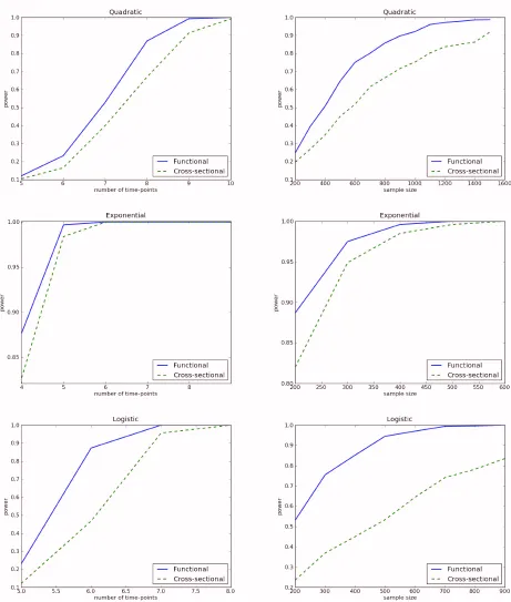
curves are in Figure 1. Several features emerge: First, power increased with the

num-ber of time points. Second, in general, the functional linear models had higher power to

detect a QTL than the cross-sectional approach, sometimes dramatically so. Third,

differ-ence in power between the functional approach and cross-sectional approach depends on

the types of genetic effect functions. We observed the largest difference in power between

the functional linear models and cross-sectional models for the logistic genetic effect

func-tion.

2

U

NSTRUCTURED COVARIANCE MATRIX

The “unstructured” covariance matrix,

Σ

3

used by Y

AP ET AL

. (2009) and used in our

simulations is given below.

Σ

3

=

⎡

⎢

⎢

⎢

⎢

⎢

⎢

⎢

⎢

⎢

⎢

⎢

⎢

⎢

⎢

⎣

0

.

72 0

.

39 0

.

45 0

.

48 0

.

50 0

.

53 0

.

60

0

.

64

0

.

68

0

.

68

0

.

39 1

.

06 1

.

61 1

.

60 1

.

50 1

.

48 1

.

55

1

.

47

1

.

35

1

.

29

0

.

45 1

.

61 3

.

29 3

.

29 3

.

17 3

.

09 3

.

19

3

.

04

2

.

78

2

.

53

0

.

48 1

.

60 3

.

29 3

.

98 4

.

07 4

.

01 4

.

17

4

.

18

4

.

00

3

.

69

0

.

50 1

.

50 3

.

17 4

.

07 4

.

70 4

.

68 4

.

66

4

.

78

4

.

70

4

.

36

0

.

53 1

.

48 3

.

09 4

.

07 4

.

68 5

.

56 6

.

23

6

.

87

7

.

11

6

.

92

0

.

60 1

.

55 3

.

19 4

.

17 4

.

66 6

.

23 8

.

59 10

.

16 10

.

80 10

.

70

0

.

64 1

.

47 3

.

04 4

.

18 4

.

78 6

.

87 10

.

16 12

.

74 13

.

80 13

.

80

0

.

68 1

.

35 2

.

78 4

.

00 4

.

70 7

.

11 10

.

80 13

.

80 15

.

33 15

.

35

0

.

68 1

.

29 2

.

53 3

.

69 4

.

36 6

.

92 10

.

70 13

.

80 15

.

35 15

.

77

⎤

⎥

⎥

⎥

⎥

⎥

⎥

⎥

⎥

⎥

⎥

⎥

⎥

⎥

⎥

⎦

.

L

ITERATURE

C

ITED

B

ANERJEE

, S., B. C

ARLIN

,

AND

A. G

ELFAND

(2004)

Hierarchical modeling and analysis for

spatial data

. Chapman & Hall.

P

ATIL

, A. (2010)

PyMC Gaussian process module Users guide

.

Y

AP

, J. S., J. F

AN

,

AND

R. W

U

(2009) Nonparametric Modeling of Longitudinal

Covari-ance Structure in Functional Mapping of Quantitative Trait Loci.

Biometrics

,

65

(4):1068–

1077.

Figure S 1

– The effect of sample size (

n

) and number of time points (

m

) on power of the

functional method using the Wald statistic. The panels on the left column show power as a

function of the number of time points, while the panels on the right column show power as a

function of sample size.

time

tr

ait

0 1 2 3 4 5 6

0.0

0

.2

0.4

0

.6

0.8

1

.0

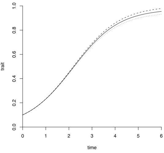
Figure S 2– Logistic mean curves under null and alternative hypotheses. The solid line cor-responds to the null hypothesis. The dashed and dotted curves correspond to the alternative hypothesis. The genetic effect is quite small, and most of the difference is in the later time points.

6

time

tr

ait

0 1 2 3 4 5 6

0.0

0

.2

0.4

0

.6

0.8

1

.0

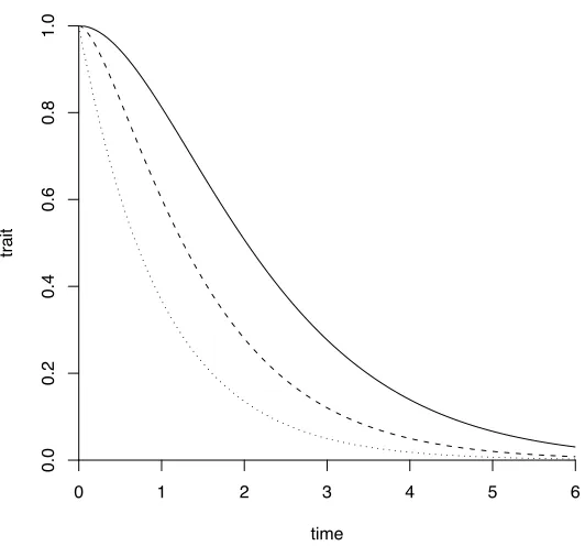
Figure S 3– Mat´ern correlation functions for three smoothness parameters. The solid line is for smoothness 2, the dashed line for smoothness 1, and dotted line for smoothness 0.5. Notice that the correlation function is not exponential, as it would be for autoregressive processes.

7

" %"&!%"%*!%"%&!%"%%**%%% "! "

'

%"& %"%* %"%& %"%%*

(%% %"&% %"%*+ %"%&& %"%%+)

)%% %"%.' %"%), %"%& %"%%)+

*%% %"&% %"%), %"%%.+ %"%%*'

+%% %"&& %"%*( %"%%-+ %"%%)+