Frequency-Domain Nonlinear Behavioral Modeling Using The Arithmetic Operator Method

(1)

HART, FRANK PATRICK. Frequency-Domain Behavioral Modeling of Nonlinear Systems Using The Arithmetic Operator Method. (Under the direction of Professor Michael B. Steer.)

A behavioral modeling environment for the rapid, high-dynamic range analysis of steady-state systems is presented. The Arithmetic Operator Method (AOM) is extended and cast in a solid mathematical framework. AOM is implemented as the AOM Toolbox within the Matlab®

(2)

(3)

by

Frank Patrick Hart

A dissertation submitted to the Graduate Faculty of North Carolina State University

in partial fullfillment of the requirements for the Degree of

Doctor of Philosophy

Electrical Engineering

Raleigh, North Carolina 2009

APPROVED BY:

Dr. K.G. Gard Dr. G. Lazzi

Dr. M.B. Steer Dr. D.W. Barlage

(4)

DEDICATION

(5)

BIOGRAPHY

(6)

ACKNOWLEDGMENTS

First and foremost I would like to thank my dissertation advisor, Dr. Michael B. Steer, for his advice throughout this work and his encouragement during its low points. I’d also like to thank the other members of my advisory committee, Drs. Doug Barlage, Gianluca Lazzi, and particularly, Kevin Gard for the many fruitful conversations that helped me to work through issues with the newer laboratory measuring equipment that he knows so well. Thanks also to Dr. Nuno Carvalho (with the Instituto de Telecommunica¸c˜oes, Universidad de Aveiro, Portugal) whose discussions on correlated and uncorrelated distortion during his sabbatical visit to NC State motivated me to nail down the correlation properties of spectral vectors based upon a vector description table; and to Dr. Yannis Viniotis, without whose remedially instructive hints in the discipline of random variables I’d have never finished that task. I’d also like to thank Dr. Jeffrey Thompson for serving as the Graduate School representative on my thesis advisory committee.

I would like to thank Ramya Mohan, Alan Victor, and Drs. Sonali R. Luniya, Nikhil M. Kriplani, Jayesh Nath, and Aaron Walker, all of whom collaborated with me in laboratory work and publications during my research assistantship. Special thanks go to Houssam Kanj, whose kind and patient assistance helped me to quickly learn a lot aboutfREEDA™_{’s internals}

as I was beginning my research work. Dr. Carlos Christoffersen, who knows fREEDA™ _best,

(7)

delivery of purchased items. Sang-Tae Bae and Dr. Meeta Yadav deserve special mention for having the intestinal fortitude to share a cubicle with me. Finally, I want to thank Jonathan Wilkerson, Greg Mazzaro, Glen Garner, Rob Harris, Justin Lowry, Vrinda P. Haridason, Jie Hu, and Chris Saunders for continuing the tradition of a stimulating doctoral research environment. The torch is now passed to you... good luck with your marathons.

I’d like to express my appreciation to the following organizations which supported the research conducted in this dissertation:

The Space and Naval Warfare Systems Center San Diego, under grant number

N6601-01-1-8921 as part of the DARPA NeoCAD Program

The U.S. Army Research Laboratory and the U.S. Army Research Office on

Mul-tifunctional Adapative Radio Radar and Sensors (MARRS) under grant number DAAD19-01-1-0496

The U.S. Army Research Laboratory and the U.S. Army Research Office as a

Mul-tidisciplinary University Research Initiative on Standoff Inverse Analysis and Ma-nipulation of Electronic Systems under grant number W911NF-05-1-0337

(8)

TABLE OF CONTENTS

LIST OF TABLES . . . xiii

LIST OF FIGURES . . . xiv

LIST OF ABBREVIATIONS . . . xix

LIST OF SYMBOLS . . . xxi

1 Introduction . . . 1

1.1 Why Nonlinear Analysis in the Frequency Domain? . . . 1

1.2 Motivations and Objectives of This Study . . . 4

1.3 Dissertation Overview . . . 6

1.4 Publications . . . 9

1.4.1 As Primary Author . . . 9

1.4.2 Not As Primary Author . . . 10

1.4.3 Planned Publications . . . 10

2 Literature Review . . . 11

2.1 Introductory Remarks . . . 11

2.2 Notation . . . 11

2.3 Time Domain Simulation . . . 12

2.4 Mixed Time and Frequency Domain Simulation . . . 12

2.5 Envelope Transient Simulation . . . 15

2.6 Nonlinear Frequency Domain Simulation . . . 15

2.6.1 Simulation with Volterra Functionals . . . 15

2.6.2 Simulation with Power Series Models . . . 17

2.6.3 Simulation with the Arithmetic Operator Method . . . 20

2.6.4 Frequency Counting Simulators . . . 25

2.6.5 Additional Developments . . . 26

2.7 Concluding Remarks . . . 26

3 The AOM Toolbox Behavioral Modeling Environment . . . 27

3.2 Mathematical Preliminaries . . . 29

3.2.1 Euler’s Formula . . . 30

3.2.2 The Sine Over Argument Function . . . 31

3.2.3 The Dirac Delta Function . . . 34

3.2.4 Fourier Transform Definition . . . 36

3.2.5 Fourier Transform of a DC Signal. . . 36

(9)

3.2.7 Fourier Transform of a Complex Exponential . . . 39

3.2.8 Fourier Transform of Sinusoidal Functions . . . 40

3.2.9 Fourier Transform of a Time-Domain Product of Functions . . . 41

3.2.10 Fourier Transform of a Time-delayed Function . . . 42

3.3 Illustrative Overview of the Arithmetic Operator Method . . . 44

3.3.1 Two-Tone Signals and Polynomial Nonlinear Transfer Function . . . 44

3.3.2 Vector Frequency Description for a Second Order Nonlinearity . . . 47

3.3.3 Introduction of Matrix Methods . . . 50

3.3.4 Vector Frequency Description for A Third Order Nonlinearity . . . 59

3.4 The Vector Frequency Description . . . 64

3.4.1 Input Signal . . . 64

3.4.2 Input Signal using the VFD . . . 64

3.4.3 Convolution of the Input using the VFD Form . . . 65

3.4.4 Modified Vector Space Properties of the VFD Table . . . 70

3.4.5 Construction of the VFD Table . . . 71

3.4.5.1 Storage Allocation . . . 71

3.4.5.2 Algorithm Description . . . 73

3.4.5.3 Duplicate Candidate VFDs . . . 76

3.4.5.4 Final Form of VFD Table . . . 76

3.4.5.5 VFD Table Construction Algorithm . . . 77

3.4.5.6 Matlab Implementation Details . . . 80

3.4.6 3-tone VFD Construction Example . . . 80

3.4.6.1 Linear Response . . . 81

3.4.6.2 Second Order Response . . . 81

3.4.6.3 Third Order Response. . . 83

3.4.6.4 3-tone VFD in Final Form . . . 89

3.5 The Spectral Vector . . . 99

3.5.1 Complex Spectral Vector . . . 99

3.5.2 Double-Sided Real Spectral Vector . . . 101

3.5.3 Single-Sided Real Spectral Vector . . . 102

3.5.4 Spectral Vector Construction Algorithm . . . 102

3.5.5 Correlation Properties of Spectral Vectors . . . 104

3.5.5.1 Uncorrelated Spectral Content . . . 107

3.5.5.2 Correlated Spectral Content . . . 110

3.5.5.3 Observations on Correlated and Uncorrelated IM Distortion . . . . 111

3.5.5.4 Spectral Correlation Theorems and Remarks . . . 113

3.6 Spectrum Mapping Table . . . 118

3.6.1 Convolution Steps and the 1-Norm Sum Test . . . 119

3.6.2 Determining The Frequency Index of the Output VFD . . . 121

3.6.3 Spectrum Mapping Table Contents . . . 123

3.6.4 Spectrum Mapping Table Construction Algorithm . . . 123

3.6.5 Matlab Implementation Details . . . 126

(10)

3.7.1 Spectrum Transform Matrix Construction Algorithm . . . 127

3.7.2 Properties of the Spectrum Transform Matrix . . . 131

3.7.3 Further Information on Eigendecomposition . . . 136

3.8 Dynamic Range of Two-Tone Tests . . . 138

3.9 Elements of FREDA2 Revisited . . . 140

3.9.1 Background . . . 140

3.9.2 One-Sided Spectrum Mapping Table . . . 140

3.9.3 1-Sided Spectrum Mapping Table Construction Algorithm . . . 144

3.9.4 One-Sided Spectrum Transform Matrix . . . 145

3.9.5 1-Sided Spectrum Transform Matrix Construction Algorithm . . . 147

3.9.6 The Exponential Function . . . 149

3.9.7 The Hyperbolic Tangent Function . . . 153

3.9.8 Summary . . . 155

4 Validation of The AOM Toolbox With a Logarithmic Amplifier Model . . . 157

4.2 Logarithmic Amplifier . . . 158

4.2.1 Circuit Analysis . . . 158

4.2.2 AOM Behavioral Model and Input Signal Form . . . 159

4.2.3 Time-Domain Input Signal . . . 163

4.2.4 Selection of Order of Spectral Truncation . . . 163

4.3 Results . . . 166

4.4 Effect of Spectral Truncation . . . 170

4.4.1 Spectral Truncation to the Third Order . . . 170

4.4.2 Spectral Truncation to the Second Order . . . 173

4.4.3 Further Discussion on Spectral Truncation . . . 175

5 Modeling the Nonlinear Response to Multitones with Uncorrelated Phase . . . 179

5.2 Measurement Apparatus . . . 180

5.2.1 Uncorrelated Phase Multitone Signal Generator . . . 180

5.2.2 Laboratory Equipment Setup . . . 181

5.2.3 Signal Chain Characterization for Simulation . . . 183

5.3 Results and Discussion . . . 185

5.3.1 Adjacent-Band IM Analysis Example . . . 188

5.3.2 Narrow-Band IM Analysis Example. . . 200

5.3.3 Phase Invariance of Simulated Average Power Computations . . . 202

5.3.4 Separating Correlated and Uncorrelated Distortion . . . 207

5.3.5 Computational Considerations . . . 211

(11)

6 Modeling the Response of a Nonlinear Amplifier to a Linear FM Chirp . . . 214

6.2 Mathematical Analysis . . . 215

6.2.1 Fourier Analysis of a Linear FM Chirp Signal . . . 215

6.2.2 Discrete Fourier Transform Scale Factors . . . 220

6.3 AOM and fREEDA Modeling Environment Setup . . . 220

6.3.1 fREEDA Circuit Models . . . 221

6.3.2 AOM Behavioral Models . . . 221

6.3.3 Butterworth Bandpass Filter Model . . . 222

6.4 Results and Discussion . . . 224

6.4.1 500 MHz Chirp Signal and Response . . . 224

6.4.1.1 MMIC Amplifier Response to a 500 MHz Chirp . . . 226

6.4.1.2 Bandpass Filtering the 500 MHz Chirp Response . . . 231

6.4.2 1 GHz Chirp Signal and Response . . . 233

6.4.2.1 MMIC Amplifier Response to a 1 GHz Chirp . . . 233

6.4.2.2 Bandpass Filtering the 1 GHz Chirp Response . . . 240

7 Modeling the Multicarrier Response of a CATV Trunk Amplifier . . . 245

7.2 The CATV Frequency Plan . . . 246

7.3 Forms of Distortion Considered . . . 247

7.4 Forms of Distortion Not Considered . . . 247

7.5 Nonlinear Amplifier Model . . . 248

7.5.1 Input Signal . . . 249

7.5.2 Gain Parameters . . . 249

7.5.3 Filter Parameters . . . 252

7.6 Results . . . 253

7.6.1 79 Channel Plan CSO/CTB Results . . . 253

7.6.1.1 79 Channel CSO Results . . . 254

7.6.1.2 79 Channel CTB Results . . . 255

7.6.2 158 Channel Plan CSO/CTB Results . . . 258

7.6.2.1 158 Channel CSO Results . . . 258

7.6.2.2 158 Channel CTB Results . . . 260

7.6.3 158 Channel Plan Filter Results . . . 260

8 Conclusion . . . 266

8.1 Summary. . . 266

8.2 Recommendations for Further Study . . . 270

(12)

Appendices . . . 293

A Z-Domain Filtering in a Transient Microwave Circuit Simulator . . . 294

A.1 Background . . . 294

A.2 The MNAM Conditioning Problem . . . 296

A.3 Z-Domain Filter Transformation . . . 299

A.4 The Butterworth Lowpass Filter Model . . . 300

A.5 The Chebychev Type I Lowpass Filter Model . . . 308

A.6 The Bandpass Filter Model . . . 311

A.7 A 1.7 GHz Coaxial Resonator Filter . . . 318

A.8 A 9 GHz Parallel-Coupled Line Filter . . . 320

A.9 Concluding Remarks . . . 323

B Uncorrelated Phase Multitone Signal Generator . . . 324

B.1 Problem Statement . . . 324

C Mathematical Foundations for AOM . . . 370

C.1 Preface. . . 370

C.2 Introduction . . . 371

C.3 Mathematical Foundation of AOM. . . 373

C.3.1 Signal Representation . . . 374

C.3.2 Multiplication as Convolution in the Frequency Domain . . . 378

C.3.3 Matrix Representation . . . 379

C.4 Arithmetic Operator Method For Real Signals . . . 381

C.4.1 Single-Sided Spectrum . . . 381

C.4.2 Definition of the Spectrum Transform Matrix . . . 383

C.4.3 Generalized Application of Transform Matrices and Vectors . . . 385

C.5 Computer-Aided Method For Developing The Spectrum Transform Matrix387 C.5.1 Basic Intermodulation Product Description Table . . . 387

C.5.2 Spectrum Mapping Table . . . 389

C.5.3 Spectrum Transform Matrix . . . 392

C.6 Discussion . . . 395

C.7 Conclusion . . . 396

C.8 Postscript - Conversion Factors in Fourier Transforms . . . 397

C.9 Postscript - Three Tone AOM . . . 398

C.10 Postscript - Automatic Development of BIPD Table Using Frequency Truncation . . . 407

D AOM Toolbox User’s Guide . . . 410

D.1 Introductory Remarks . . . 410

D.2 Installation . . . 410

D.3 Usage Overview . . . 411

D.4 Application Example . . . 414

D.4.1 Problem Description . . . 414

D.4.2 Analysis of Mixer A . . . 416

D.4.3 Ideal Bandpass Filtering of Mixer A Output . . . 421

(13)

D.4.5 Output Processing . . . 426

D.5 Known Limitations and Workarounds . . . 427

D.6 Concluding Remarks . . . 427

E FREDA2 Transcendental Function Examples . . . 429

E.1 Introductory Remarks . . . 429

E.2 Exponential Function . . . 429

E.2.1 Discussion and Results . . . 429

E.2.2 AOM Exponential Driver Script . . . 432

E.2.3 AOM Exponential Function . . . 435

E.3 Hyperbolic Tangent Function . . . 437

E.3.1 Discussion and Results . . . 437

E.3.2 AOM Hyperbolic Tangent Driver Script . . . 440

E.3.3 AOM Hyperbolic Tangent Function . . . 443

F Listings of MATLAB Codes . . . 446

F.1 Introductory Remarks . . . 446

F.2 Listings of the AOM Toolbox Codes . . . 446

F.2.1 AOM VFD Table Generation Function . . . 446

F.2.2 AOM VFD Count Estimation Function . . . 456

F.2.3 AOM Int8 Column Permutation Function . . . 459

F.2.4 AOM Int8 Matrix Multiplication Function . . . 461

F.2.5 AOM Spectral Vector Creation Function . . . 463

F.2.6 AOM Spectrum Mapping Table Function . . . 466

F.2.7 AOM Spectrum Transform Matrix Function . . . 475

F.2.8 AOM Sparse Block Evaluation Function . . . 479

F.2.9 AOM Unit DC Spectral Vector Function . . . 483

F.2.10 AOM Ideal Bandpass Filter Function . . . 485

F.2.11 AOM Butterworth Bandpass Filter Function . . . 488

F.2.12 AOM Butterworth Lowpass Filter Function . . . 492

F.2.13 AOM Spectral to Complex Vector Function . . . 495

F.2.14 AOM Complex to Spectral Vector Function . . . 497

F.2.15 AOM Phasor Conversion Function . . . 499

F.2.16 AOM Power to Voltage Conversion Function . . . 500

F.2.17 AOM Voltage to Power Conversion Function . . . 501

F.3 Listings of Matlab Codes used in Chapter 3 . . . 502

F.3.1 AOM Dynamic Range Demonstration Script . . . 502

F.3.2 FFT Dynamic Range Reference Script . . . 504

F.3.3 Dynamic Range Plotting Script . . . 507

F.4.1 Logarithmic Amplifier Driver Script . . . 508

F.4.2 Logarithmic Amplifier Function . . . 512

F.4.3 Spice Data Import Function . . . 517

F.4.4 VFD to LaTeX Export Function . . . 519

(14)

F.5.1 Uncorrelated Phase Multitone Driver Script . . . 521

F.5.2 Uncorrelated Phase Multitone Function . . . 522

F.6.1 Broadband Chirp Modeling Driver Script . . . 541

F.6.2 Broadband Chirp Modeling Function . . . 543

F.7.1 Multicarrier CATV Modeling Driver Script . . . 549

(15)

LIST OF TABLES

Table 2.1 Mixer BIPD Table built using the method of Rhyne . . . 19

Table 2.2 OutputIndex Vector generated by method of Carvalho & Pedro . . . 25

Table 3.1 1-Norm Sort VFD Table for 2 Tones in a 2nd Order Nonlinearity . . . 48

Table 3.2 1-Norm Sort VFD Table for 2 Tones in a 3rd Order Nonlinearity . . . 59

Table 3.3 1-Norm Sort 1-Side VFD Table for 3 Tones in a 3rd Order Nonlinearity . . 90

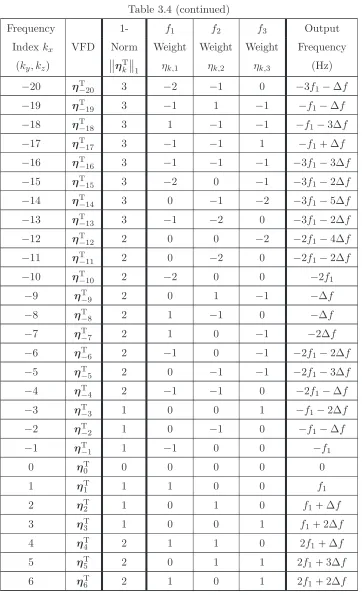
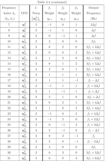
Table 3.4 1-Norm Sort 2-Side VFD Table for 3 Tones in a 3rd Order Nonlinearity . . 91

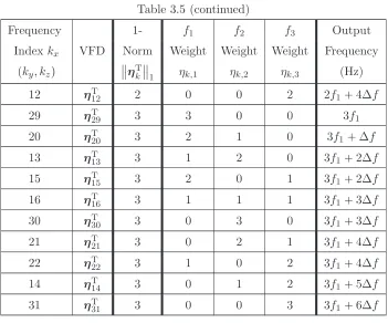
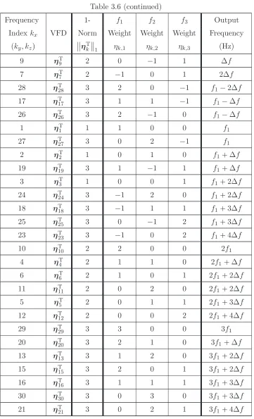
Table 3.5 Frequency Sort 1-Side VFD Table for 3 Tones in a 3rd Order Nonlinearity 94 Table 3.6 Frequency Sort 2-Side VFD Table for 3 Tones in a 3rd Order Nonlinearity 95 Table 3.7 1-Sided Version of Table 3.1 on page 48. . . 142

Table 4.1 Log Amplifier VFD Table for 2 Tones in a 5th Order Nonlinearity . . . 164

Table 4.2 Log Amplifier VFD Table for 2 Tones in a 3rd Order Nonlinearity . . . 171

Table 4.3 Log Amplifier VFD Table for 2 Tones in a 2nd Order Nonlinearity . . . 173

Table 5.1 Numbers of phasors averaged at adjacent-band IM frequencies.. . . 189

Table 5.2 Measured frequencies of carrier oscillation for narrow-band IM analysis. . . 200

Table 5.3 Numbers of phasors averaged at in-band IM frequencies. . . 202

Table 5.4 Costs of computation for uncorrelated multitones. . . 211

Table 6.1 Amplifier Coefficients . . . 222

Table 7.1 Gain Parameters . . . 250

Table 7.2 Filter Block Parameters . . . 252

Table 7.3 Costs of computation for CATV amplification. . . 264

Table 8.1 Comparison of AOM to other methods . . . 268

Table A.1 z-domain Butterworth lowpass filter block coefficient definitions . . . 305

Table A.2 Transfer function denominator coefficients . . . 313

Table A.3 Bandpass filter block coefficient definitions . . . 315

Table B.1 Bill of Materials for 3-oscillator Assembly in Figure B.2 . . . 326

Table C.1 BIPD Table for spectrum of Figure C.3 . . . 389

Table C.2 Spectrum Mapping Table entry . . . 390

Table C.3 Portions of the Spectrum Mapping Table . . . 391

Table C.4 BIPD Table for 3rd Order Non-Linear Transfer Function . . . 408

Table D.1 Mixer A VFD Table for 3 Tones in a 2nd Order Nonlinearity . . . 418

(16)

LIST OF FIGURES

Figure 2.1 Circuit partitioning for Harmonic Balance. . . 13

Figure 2.2 Frequencies of interest in a mixer. . . 18

Figure 3.1 Complex contour integral ofeαz {z.. . . 32

Figure 3.2 I 1, the 1 st _{step of spectral vector discrete convolution. . . 52}

Figure 3.3 I 2, the 2 nd _{step of spectral vector discrete convolution. . . 52}

Figure 3.4 I 6, the 6 th _{step of spectral vector discrete convolution. . . 53}

Figure 3.10 Spectrum Transform Matrix constructed from the 25 convolution steps. . 57

Figure 3.11 Spectrum Transform Matrix created from (3.135). . . 63

Figure 3.12 Number of 1-sided VFD Table entries for givenQ,N. . . 72

Figure 3.13 Storage required for minimal data structures for a given problem. . . 72

Figure 3.14 Upper circulant shift permutation matrixP. . . 74

Figure 3.15 Upper circulant shift permutation matrixP2_{. . . 75}

Figure 3.16 Row-flipping permutation matrixJ. . . 77

Figure 3.17 Quadrature modulation of two real input signals. . . 100

Figure 3.18 I KQ, 1 st _{atomic multiplication. . . 119}

Figure 3.19 I 2KLQ, 1 st _{valid atomic product. . . 120}

Figure 3.20 I 2KQ, step with valid atomic multiplication products. . . 120

Figure 3.21 I 2K Q, step with valid atomic multiplication products. . . 121

Figure 3.22 I 4KQ, final convolution step with valid products. . . 121

Figure 3.23 I 4K1, the final convolution step – with invalid products. . . 122

Figure 3.24 2-Sided Spectrum Transform Matrix Stamps. . . 128

Figure 3.25 Spectrum Transform Matrix from the example in Section 3.3.3. . . 131

Figure 3.26 Spectrum Transform Matrix for a conjugate symmetric two-tone signal. . 132

Figure 3.27 tanhpxq and Cann models fors2,3,4. . . 135

Figure 3.28 Two tone dynamic range of the AOM Toolbox vs. the FFT. . . 138

Figure 3.29 Relative Error in the approximation of exppxq forn6,7,8. . . 149

Figure 3.30 Relative errors in function approximations. . . 154

Figure 4.1 Circuit diagram of an ideal logarithmic amplifier. . . 158

Figure 4.2 Results of simulating the logarithmic amplifier. . . 167

(17)

Figure 4.6 Results of spectral truncation at the 3rd _{order. . . 172}

Figure 4.7 Relative error for 3rd _{order spectral truncation. . . 172}

Figure 4.8 Results of spectral truncation at the 2nd _{order.. . . 174}

Figure 4.9 Relative error for 2nd _{order spectral truncation. . . 175}

Figure 4.10 Iteration tolerance for at various orders of spectral truncation. . . 176

Figure 4.11 Actual error at various orders of spectral truncation. . . 176

Figure 5.1 Simplified block diagram of a three oscillator assembly. . . 181

Figure 5.2 Block diagram of the multitone system of 5 three-tone assemblies. . . 182

Figure 5.3 Block diagram of the laboratory setup. . . 182

Figure 5.4 Laboratory photo of measurements in progress. . . 182

Figure 5.5 Block diagram of the uncorrelated phase signal measurement chain. . . 184

Figure 5.6 Characterized average output power from 15 oscillators before combining.186 Figure 5.7 Characterized average output power from 15 oscillators after combining.. 187

Figure 5.8 Simulated and measured results for adjacent-band IM. . . 189

Figure 5.9 Detail view of the linear response. . . 191

Figure 5.10 Detail view of the lower adjacent-band response. . . 192

Figure 5.11 Results of enforced correlation simulations 1-10. . . 193

Figure 5.14 Results of averaging 8 enforced correlation simulations. . . 196

Figure 5.15 Average of Enforced Correlation Phase Regimes 1–16. . . 196

Figure 5.16 Average of Enforced Correlation Phase Regimes 1–30. . . 197

Figure 5.17 Linear response detail of the average. . . 197

Figure 5.18 Left adjacent IM band response detail of the average. . . 198

Figure 5.19 Relative error between ensemble and a single simulation. . . 199

Figure 5.20 Simulated and measured results for narrowband IM. . . 201

Figure 5.21 Average PSD results from 30 simulations with 1-sided vectors. . . 203

Figure 5.22 Absolute difference between min and max powers for 1-sided simulations. 204 Figure 5.23 Average PSD results from 30 simulations with 2-sided vectors. . . 205

Figure 5.24 Absolute difference between min and max powers for 2-sided simulations. 206 Figure 5.25 Adjacent and co-channel band view for measured source amplitude. . . 207

Figure 5.26 Magnification of the co-channel band view for measured source amplitude.208 Figure 5.27 Adjacent and co-channel band view for average source amplitude. . . 209

Figure 5.28 Magnification of the co-channel band view for average source amplitude. 210 Figure 6.1 Block diagram of the simulated radar transmission chain. . . 221

Figure 6.2 Attenuation (in dB) of the bandpass filters. . . 223

Figure 6.3 Phase change (in degrees) introduced by the bandpass filters. . . 223

Figure 6.4 Magnitude of the 500 MHz linear FM chirp input. . . 224

Figure 6.5 Magnitude detail of the peak of the 500 MHz LFM chirp input. . . 225

Figure 6.6 Phase of the 500 MHz linear FM chirp input. . . 225

Figure 6.7 Magnitude of the MMIC outputWpfq in the chirp range. . . 227

(18)

Figure 6.9 Magnitude of the whole-spectrum MMIC outputWpfq. . . 229

Figure 6.10 Detail view of the 7th _{harmonic of the} _f_REEDA™ _{MMIC output} _W pfq. . . 230

Figure 6.11 Detail view of the 3rd _{harmonic output} _W pfq. . . 230

Figure 6.12 Magnitude of the adjacent band outputs. . . 231

Figure 6.13 Magnitude of the 3rd _{harmonic outputs. . . 232}

Figure 6.14 Magnitude of the whole-spectrumfREEDA™ _output _Y pfq. . . 232

Figure 6.15 Magnitude of the 1 GHz linear FM chirp input. . . 234

Figure 6.16 Magnitude detail of the peak of the 1 GHz LFM chirp input. . . 235

Figure 6.17 Phase of the 1 GHz linear FM chirp input. . . 235

Figure 6.18 Magnitude of the MMIC outputWpfq in the chirp range. . . 236

Figure 6.19 Magnitude detail of the MMIC chirp peak output ofWpfq. . . 237

Figure 6.20 Magnitude of the whole-spectrum MMIC outputWpfq. . . 239

Figure 6.21 Detail view of the 7th _{harmonic of the} _f_REEDA™ _{MMIC output} _W pfq. . . 239

Figure 6.22 Detail view of the 3rd _{harmonic output} _W pfq. . . 241

Figure 6.23 Magnitude of the adjacent band outputs. . . 241

Figure 6.24 Magnitude of the 3rd _{harmonic outputs. . . 242}

Figure 6.25 Magnitude of the whole-spectrumfREEDA™ _output _Y pfq. . . 243

Figure 7.1 Behavioral model for the CATV amplifier. . . 248

Figure 7.2 Nonlinearity Distortion Parameters used to deriveG2 and G3. . . 250

Figure 7.3 Nonlinearity Distortion Parameter D2pfq. . . 251

Figure 7.4 Nonlinearity Distortion Parameter D3pfq. . . 251

Figure 7.5 Magnitude Response ofK1pfq, K2pfq, andK3pfq. . . 252

Figure 7.6 Phase response of filtersK1pfq, K2pfq,and K3pfq. . . 253

Figure 7.7 CSO power spectral density for a 79 channel plan. . . 254

Figure 7.8 1.25 MHz CSO beats for a 79 channel plan. . . 255

Figure 7.10 CTB power spectral density for a 79 channel plan. . . 257

Figure 7.11 CTB beats for a 79 channel plan. . . 257

Figure 7.12 CSO power spectral density for a 158 channel plan. . . 258

Figure 7.15 CTB power spectral density for a 158 channel plan. . . 260

Figure 7.16 CTB beats for a 158 channel plan. . . 261

Figure 7.17 Effect of filtering the linear output for a 158 channel plan. . . 262

Figure 7.18 Effect of filtering the 2nd _{order harmonic for a 158 channel plan. . . 262}

Figure 7.19 Effect of filtering the 3rd _{order harmonic for a 158 channel plan. . . 263}

Figure A.1 Filter synthesis limitations of a leading commercial simulator. . . 296

Figure A.2 Two-stage ladder circuit with ill-conditioned MNAM. . . 297

Figure A.3 Condition number of MNAM for the two-stage ladder circuit. . . 298

Figure A.4 Typical parameters for a Butterworth lowpass filter. . . 301

Figure A.5 Discrete-time lowpass Butterworth filter in cascade form . . . 305

(19)

Figure A.7 Discrete-time filter block permitting Newton iteration . . . 307

Figure A.8 Discrete-time filter block at initial iterate of time step . . . 308

Figure A.9 Typical parameters for a Chebychev Type I lowpass filter. . . 309

Figure A.10 Typical parameters for a bandpass filter. . . 312

Figure A.11 Discrete-time bandpass filter in cascade form. . . 314

Figure A.12 Typical discrete-time filter block in canonical form. . . 317

Figure A.13 Frequency response results for a 5-section coaxial filter. . . 318

Figure A.14 Response of simulated filter to a Linear FM chirp signal. . . 319

Figure A.15 Block diagram of the laboratory measurements setup. . . 320

Figure A.16 Layout of the microstrip patterns in the fabricated filter. . . 321

Figure A.17 Measured and simulated results near the lower edge of the passband. . . 322

Figure B.1 Schematic of circuitry supporting one VCO. . . 329

Figure B.2 Block Diagram of an assembly of three oscillators. . . 330

Figure B.3 Photo of a 3 oscillator assembly. . . 331

Figure B.4 Results of two injection pulling experiments. . . 334

Figure B.5 Histogram of oscillator frequency locations for Assembly 1. . . 336

Figure B.6 Amplitude and Frequency Running Standard Deviation for Assembly 1. . 337

Figure B.7 Instantaneous and Running Average Amplitude for Assembly 1. . . 338

Figure B.8 Instantaneous and Running Average Frequency for Assembly 1. . . 339

(20)

Figure C.1 An ideal multiplier withyptqxptqzptq. . . 373

Figure C.2 Spectral representation of a three-tone signal. . . 375

Figure C.3 The approximate spectrum resulting from the excitation byf1 and f2. . . 388

Figure C.4 Generic Double-Sided spectrum with frequencies identified.. . . 405

Figure D.1 Typical analysis flow for solving a problem with the AOM Toolbox. . . 413

Figure D.2 Microwave mixer schematic model. . . 415

Figure D.3 Microwave mixer analysis model. . . 415

Figure D.4 IF output from Mixer A. . . 420

Figure D.5 RF (linear) output from Mixer A. . . 420

Figure D.6 2nd _{order harmonic and IM output from Mixer A. . . 421}

Figure D.7 IF output from Mixer A. . . 422

Figure D.8 IF output from Mixer B. . . 425

Figure D.9 RF (linear) output from Mixer B. . . 425

Figure D.10 2nd _{order harmonic and IM output from Mixer B. . . 426}

Figure E.1 Exponential response to 2 tones with 2nd _{order truncation. . . 430}

Figure E.2 Detail view of 2nd order truncated exp() response. . . 431

Figure E.3 Exponential response to 2 tones with 3rd _{order truncation. . . 431}

Figure E.4 Detail view of 3rd _{order truncated exp() response. . . 432}

Figure E.5 Hyperbolic tangent response to 2 tones with 2nd order truncation. . . 438

Figure E.6 Detail view of 2nd _{order truncated exp() response. . . 439}

Figure E.7 Hyperbolic tangent response to 2 tones with 3rd _{order truncation. . . 439}

(21)

LIST OF ABBREVIATIONS

AC Alternating Current: Within the context of spectral analysis, refers to spec-tral content not at DC

ADS Advanced Design System: A microwave computer-aided design software en-vironment available from Agilent

AOM Arithmetic Operator Method: Frequency-domain convolution simulation method

BIPD Basic Intermodulation Product Description: User-select tabular weightings of incommensurate input frequencies

CATV Cable TV: System of multi-channel video content delivered over coaxial cable or fiber

CDMA Code Division Multiple Access: A signalling scheme for wireless communica-tions used primarily in cellular devices

CSO Composite Second Order: Collection of 2nd order intermodulation of 2 dis-tinct frequencies mapping to a disdis-tinct frequency

CTB Composite Triple Beat: Collection of 3rd _{order intermodulation involving 3}

distinct frequencies

DC Direct Current: Within the context of spectral analysis, refers to spectral content at 0 Hz

FFT Fast Fourier Transform: A fast method of computing the Discrete Fourier Transform

FM Frequency Modulation: Constant-amplitude, variable-phase modulation method

GaAs Gallium Arsenide: A material used to create high-speed semiconductor de-vices

HB Harmonic Balance: A mixed time/frequency domain simulation method

I-FFT Inverse Fast Fourier Transform: A fast method of computing the Inverse Discrete Fourier Transform

(22)

MESFET Metal Epitaxial Semiconductor Field Effect Transistor: A transistor created with a metal semiconductor gate instead of a bipolar junction

MNAM Modified Nodal Admittance Matrix: An admittance matrix for nodal circuit analysis which includes voltage sources

PHEMT Pseudomorphic High Electon Mobility Transistor: A high-speed transistor created by joining two materials without a doped bandgap

Spice Simulation Program with Integrated Circuit Emphasis: Simulation Program with Integrated Circuit Emphasis

(23)

LIST OF SYMBOLS

AH Hermitian of matrix A. . . 132

Aq Amplitude (Volts) of theqth sinusoid when using AOM . . . 20

B 3 dB passband of a bandpass filter. . . 297

β Multiplicative complex constant in correlation computations . . . 108

bn Coefficients of the polynomial transfer function yptq. . . 22

Operator denoting the convolution of two quantities.. . . 21

Cpq

x Spectral vector resulting from repeated convolution times . . . 58

dB Decibel, a logarithmic power measurement scale . . . 14

δpq Dirac delta function . . . 34

D3pfq Third-order CATV nonlinearity parameter. . . 249

D2pfq Second-order CATV nonlinearity parameter . . . 249

e0 Unit spectral vector corresponding to DC . . . 22

Ergpφqs Expected value of the functiongpφq. . . 109

H Set of VFDs forming a VFD Table. . . 70

ηT_k kth _{VFD appearing in a VFD table, a row vector of integers . . . 47}

H

Negative frequency portion of a VFD Table . . . 77

H Estimated storage required to hold VFD table under construction. . . 71

em˜ Iteration error in time domain . . . 162

J Exchange matrix . . . 77

fc Center frequency using the indexing scheme of Carvalho and Pedro . . . 24

FH VFD Table in frequency-sort order, symmetric about DC when 2-sided . . . 77

F1

r s Inverse Fourier transform operation . . . 36

fin Vector of input frequencies (Hz) . . . 47

(24)

Means for any orfor all as ink. . . 19

F

ðñ Denotes functions forming a Fourier transform pair . . . 36

fΦpφq Probability density function of φ. . . 109

fq Frequency (Hz) of theqth sinusoid when using AOM . . . 20

Fr s Fourier transform operation . . . 21

Γkk kth element of phasor delay matrix Γn. . . 22

Γn Diagonal matrix of delay phasors corresponding to delay τn. . . 22

An Associate memory (hash table) that returns VFD location in H . . . 76

Hnc Temporary matrix of candidate VFDs during VFD Table construction . . . . 74

I Identity matrix . . . 25

I Number of convolution index steps in discrete convolution . . . 119

Ipfq In-phase baseband data stream in frequency-domain . . . 100

˜

Ipfq In-phase modulated data in frequency-domain . . . 100

Imrs Imaginary part of a complex argument . . . 32

P Means is a member of the set. . . 12

kk 8

Infinity norm of a vector . . . 12

I Field of integers; I1Q

denotes a row vector of integers . . . 69

iptq In-phase baseband data stream in time-domain . . . 100

 The imaginary number . . . 12

K Number of entries in a VFD table . . . 7 ˆ

Kn Estimate of the number of VFD table entries at nonlinear order n. . . 71 ˆ

K Estimate of the number of VFD table entries over all nonlinear orders . . . . 71

kx Frequency index for vector X. . . 48

ky Frequency index for vector Y. . . 48

kz Frequency index for vector Z. . . 48

Λ Diagonal matrix appearing in Eigendecomposition . . . 134

(25)

µ Chirp rate in a radar transmission system . . . 215

N Maximum nonlinear order of a transfer function . . . 18

NH VFD Table in one-norm sort order, symmetric about DC when 2-sided . . . . 77

|H| Number of distinct elements in a VFD Table . . . 71

|Hn| Number of distinct VFD table entries at nonlinear ordern. . . 71

ωa Continuous-time or analog frequency (rad/sec) . . . 299

ω0 Center frequency of a bandpass filter (rad/sec) . . . 297

ωp Pre-warped discrete-time equivalent of omegaa. . . 299

kk

1 1-norm of a vector . . . 12

P Permutation matrix . . . 73

φ_in Vector of input phases (radians) . . . 49 φq Phase (Radians) of theqth sinusoid when using AOM . . . 20

ψ Scaling factor for ladder filter circuits. . . 296

Q Number of independent input tones . . . 24

Qpfq Quadrature baseband data stream in frequency-domain . . . 100

˜

Qpfq Quadrature modulated data in frequency-domain . . . 100

qn Dummy index variable in multitone summation expressions . . . 46

qptq Quadrature baseband data stream in time-domain . . . 100

Cpnq

xk Phasor component kof C

pnq

x . . . 62 Rers Real part of a complex argument . . . 32

Πpq Rectangular function . . . 35

RXY Complex correlation of quantities X and Y . . . 107

σF Running frequency standard deviation. . . 332

τn Order-dependent time delays in the polynomial transfer function yptq. . . 22

θ Phase angle . . . 30

U Unitary matrix, whereUH_U

I. . . 133

r

(26)

u

C Closed contour integral along path C . . . 32 Vbe Base-to-emitter junction voltage . . . 158

VT Thermal voltage of a BJT . . . 159

W Numerator vector in rational polynomial . . . 134

Qpfq Sum of in-phase and quadrature modulated data in frequency-domain . . . 100

Xpfq Fourier transform of xptq. . . 21

Xq Phasor form of the qth sinusoid, i.e. Xq Aqe

φq _{. . . 20}

XÆ

q Complex conjugate of phasorXq . . . 20 X Spectral vector corresponding to Xpfq. . . 21

xptq Time-domain function designating a collection of sinusoids . . . 20

Tx Spectrum transform matrix created from X. . . 21

(27)

Chapter 1

Introduction

1.1 Why Nonlinear Analysis in the Frequency Domain?

Computer simulation is used in many fields of theoretical and applied science, by both re-searchers and practitioners. Simulation is used to model things where it is impossible to make analogous scale models — such as planetary atmospheric behavior or the movements of celestial bodies — as well as situations where computer modeling (and subsequent revision as an inte-gral part of the design flow) prior to fabrication of the real thing is far more economical than the alternative approach oftrial and error prototype model construction with repeated design revisions. Fabrication of most semiconductor device designs is an example of the latter case where computer simulation is used. In most cases, behavioral models of real nonlinear systems are simulated with time as the independent variable. That is, most models of real systems are simulated with a view to predicting the response of the system if it were started at some point in time and then subsequently observed. Within the computer simulation environment, the starting moment is usually set to zero, the system’s behavior is initialized to some known state, and the system’s behavior going forward is observed. This is known astransient or time-domain simulation, and simulation environments operating in the time-time-domain usually operate by numerically solving a set of discretized nonlinear differential equations subject to whatever initial values are given.

(28)

in addition to the three-dimensional spatial coordinates it is a physical dimension in which humans live and it is a dimension which they can visually observe. With the assistance of measuring devices they can observe and measure time differences beyond human observational abilities. There are, however, other domains upon which scientific inquiry and experimental observation may be based, but since these domains are alien to human existence, they are not as popular. The frequency-domain is one such domain. The frequency-domain is one of inverse observational characteristics to the time-domain: Impulsive time-domain behavior such as noise spikes appears aswhite noise that spans the entire frequency domain as a constant value, while pairs of positive and negative impulsive spikes (at the same absolute frequency value) in the frequency-domain correspond to an infinitely-oscillating sinusoidal signal (unless the frequency at which the frequency-domain impulse occurs is zero, which is then just a constant DC signal). Where it has proven useful, sophisticated measuring devices — such as spectrum analyzers — which produce visual output in the frequency-domain have also been produced, although these devices necessarily operate in the time-domain and post-process measurements into the frequency-domain.

(29)

frequency happens in a small fraction of the time required to simulate the baseband. A typical modulation or demodulation circuit simulated over just a few baseband frequency periods will result in millions or even billions of periods of oscillation in the modulated signal. Note that this inefficiency is an inherent consequence of using time-domain simulation techniques to simulate theintended nonlinear behavior of a particular circuit – and the existence of this inefficiency has spurred interest in hybrid simulator environments that combine time-domain and frequency-domain simulation to increase computational efficiency while still obtaining useful output for evaluating the simulated model’s conformance to performance metrics.

In addition to problems where the use of time-domain simulation is simply inherently inefficient, there are a few other classes of problems which are simply intractable for simulation in the time-domain. One example is the problem of frequency planning or frequency spectrum allocation, which is ultimately the assignment of carrier frequencies in multi-carrier systems with the objective of minimizing the in-band distortion products produced by nonlinear inter-actions (usually caused by nonlinear amplification) of two or more carriers for other bands. This problem is well-known in the field of satellite communications, where very broad amplification bandwidth spanning several frequency octaves combined with narrowband frequency assign-ments causes concern with the harmonic distortion of carriers in the lower adjacent frequency octave. A similar problem exists in other multicarrier systems, such as television broadcasting and cellular communications. In these realms, a related problem is the performance of nonlinear amplifiers for a given frequency plan. In some cases — Code Division Multiple Access (CDMA) cellular communications, for example — performance metrics are defined by signal inputs in the time-domain with output measurements in the frequency-domain, and in these cases, one of the hybrid time- and frequency-domain simulator environments that perform harmonic balance analysis is appropriate. However, there are cases where the signal input for performance met-rics is defined in the frequency-domain and the outputs are measured in the frequency-domain. Cable and satellite television broadcasting is an example. Here, independent carriers — with no firmly defined time-domain behavioral definition for their modulated baseband signals — are combined and amplified by a nonlinear amplifier, either for rebroadcast by a satellite down-link or for redriving down a cable television network trunk cable. Transient simulation is thus useless and simulation — when it is used at all — must be done in the frequency-domain.

(30)

perfor-mance metric is defined in the frequency-domain, there is a possibility that numerical limita-tions in the simulator environment may tend to preclude using an input in the time-domain. For example, if very low-level signals defined in the time-domain (for example, simulations of radio signals received from space and processed through low-noise amplifiers in a temperature-controlled environment — usually with the amplifier immersed in liquid nitrogen) are processed through a nonlinearity and then the output is transformed to the frequency-domain using the Fast Fourier Transform (FFT), the resulting signal may be very close to the numerical noise floor such that invalid results are obtained. In these cases, numerical computation must be minimized and thus the use of the FFT must be avoided, which leads to defining the input in the frequency-domain.

In general, circuit simulation is performed predominantly in the time-domain. How-ever, there are cases where frequency-domain simulation is preferable, and others where it is the only available simulation option. The growth of the commercial offerings in the hybrid simula-tion environments is a testament to the pragmatism of engineers for choosing the environment best suited to the needs of their problems, but also indicates an increasing acceptance for using the frequency-domain as an alternative. There is, however, a dearth of nonlinear simulation environments that operate solely in the frequency-domain. The body of work presented here is a contribution to remedying this situation.

1.2 Motivations and Objectives of This Study

(31)

contemporary commercial simulators are limited to twelve or fewer input tones.

In the realm of simulation entirely in the frequency domain, circuit simulator engines based on power series analysis have been used to simulate memoryless nonlinearities and sys-tems with order-dependent time delays. In these simulators, it was thus possible to simulate more strongly nonlinear systems with larger-signal inputs. However, these simulators used ad-hoc techniques to tabulate the frequencies at which output signals would occur, and reported results were typically oriented toward characterizing two-tone, 3rd _{order intermodulation}

am-plifier responses. No attempt was made in these simulator engines to handle large numbers of input tones. In an exception to this generality, one group of researchers implemented a rigor-ous technique to identify the set of output frequencies based upon a set of uniformly-spaced input tones. Researchers working on implementing Volterra series analysis in frequency domain simulators have been able to simulate complex weakly nonlinear systems containing memory. However, these efforts have also been limited to low orders of nonlinearity and low numbers of input tones because of the complexity of extracting the Volterra kernels for incorporation into the simulator engine.

(32)

for investigating problems beyond the capability of existing HB simulator environments and other existing frequency domain simulator environments.

1.3 Dissertation Overview

The literature on computer-aided simulation of electrical and electronic circuits is vast, dating back to the 1950s. No single review could do it justice. Thus the objective of Chapter 2 is em-phasizing literature discussing simulator environments, with special emphasis on the literature about simulators operating in the frequency domain. The chapter begins with brief coverage of noteworthy literature about time domain and HB simulators, discusses some efforts in the realm of simulators based on Volterra series analysis, and then delves more deeply into the literature on frequency domain simulators. The origins of the Basic Intermodulation Product Description (BIPD) and Spectrum Mapping tables and Arithmetic Operator Method (AOM) as implemented in theFREDA2 circuit simulator are described. The novel technique that iden-tified output frequencies based on a set of uniformly-spaced input tones is also described. Other efforts to identify output frequency sets are also noted.

Chapter 3 begins with the mathematical foundations for the Arithmetic Operator Method in the form of a select set of Fourier transforms of generalized functions. The founda-tion begins with Euler’s formula, followed by a discussion of properties of the sinx{x function,

(33)

correlation properties of spectral vectors created from uncorrelated phase multitone inputs are given. The peculiar phenomenon of correlated intermodulation distortion occurring at higher power levels than uncorrelated distortion due to interaction with a previously rectified Direct Current (DC) signal is illustrated in the 3-tone analytical example. The Spectrum Mapping table (which drives the creation of the spectrum transform matrix) is then described, with a description of an improved algorithm (versus previous work) which reduces the computational complexity of creating the spectrum mapping table from OpK

3

q to OpK 2

q, where K is the

number of entries in the VFD table. The Spectrum Transform matrix and its construction al-gorithm are then described, with an emphasis on the exploitation of the sparsity of the matrix in its construction. An important discovery that two-sided complex-conjugate spectral vectors yield Hermitian spectrum transform matrices is then described and proved. This discovery provides a path for the use of eigendecomposition as an alternative to the usual linear algebra methods for solving systems of equations, and may well be theonly way to solve problems with rational polynomial transfer functions when the input is a multitone signal with uncorrelated phase. A final section derives the one-sided version of the Arithmetic Operator Method, first introduced by Chang, as a special case of the two-sided complex version when the input signal is purely real. The final section also expands on the discussion of implementing exponential and hyperbolic functions using the Arithmetic Operator Method, filling in some details that Chang did not include in his work.

Chapter 4 validates the functions of the AOM Toolbox by simulating the response of a logarithmic amplifier to a two-tone sinusoidal input signal. The nonlinearly-created output phasors of the AOM Toolbox simulation are expanded in the time domain and compared to the results of a pure time-domain simulation of the input signals using Matlab® _{natural logarithm}

function to perform the computations. Results from a PSpice simulation of a circuit netlist are also shown and compared in order to have a reference independent from the Matlab®_computing

environment. The effects of spectral truncation — a necessity whenever when transcendental transfer functions are simulated — are illustrated.

(34)

inputs thanks to the ability of the VFD table to permit more than one spectral vector element at each numeric frequency. When correlation is enforced by the AOM Toolbox, it is possible to observe the effect of input phase on intermodulation power in the adjacent bands and note that it is similar to the results produced by environments that enforce correlation. When the AOM Toolbox treats the uncorrelated phase inputs (i.e. inputs where the phases are independent, identically distributed random variables [1, 2]) properly however, it is possible to predict the average power of the output spectrum from asingle simulation, something which is has been demonstrated in only one other instance [3] — but an instance, unfortunately, where measurements used phase-locked sources as contrasted to the unlocked sources used in this work. Recovery of the correlated and uncorrelated co-channel intermodulation power is also possible in a single simulation, and results of this investigation are given.

Chapter 6 explores an application of AOM Toolbox to simulating a broadband linear Frequency Modulation (FM) chirp [4] through a radar transmission chain. Beginning with the analytical description of the linear FM chirp in the frequency domain (a Fresnel integral form), a discretized version of the input signal will be created in the frequency domain and processed through the chain in the AOM Toolbox. Results are compared to those produced from the FFT of thefREEDA™ _{output of the same chain in the time domain for inputs with 500 MHz and 1}

GHz chirp bandwidths.

Chapter 7 addresses the realm of multicarrier broadband transmissions modeling, for which there are presently no simulation tools whatsoever. Thus a frequency domain behavioral modeling environment capable of handling a large number of tones would prove quite useful in these fields. One commercial application is to the prediction of Intermodulation (IM) in Cable TV (CATV) distribution networks. An illustrative use of the AOM Toolbox to predicting the Composite Second Order (CSO) and Composite Triple Beat (CTB) [5] distortion produced by a hypothetical amplifier is given. (For lack of broadband amplifier models, comparison to measured results will not be possible.) A 79-channel case furnishes results that can compared to previous reports in the literature, while a 158-channel case produces results not previously reported.

(35)

models, followed by descriptions of Butterworth and Chebychev filter blocks that may be syn-thesized into an arbitrary number of cascaded blocks so as to facilitate the creation of filters of arbitrary order for use in transient simulation. Results of modeling two filters are given.

Appendix B describes the design and characterization of the uncorrelated phase mul-titone signal generator which was measured in Chapter 5.

Appendix C encapsulates the content of the first publication by the author (as lead author) on an early prototype implementation of the AOM Toolbox in Matlab®_{. The work}

disclosed in this publication has been so thoroughly eclipsed by the subsequent developments in the AOM Toolbox codes that it could not be effectively included in the main body of the dissertation.

Appendix D provides a User’s Guide to the AOM Toolbox with a specific application to the analysis of two cascaded mixer stages that perform a heterodyne demodulator function.

Appendix E furnishes code listings with embedded documentation.

1.4 Publications

1.4.1 As Primary Author

1. F.P. Hart, D.G. Stephenson, C.R. Chang, K. Gharaibeh, R.G. Johnson, and M.B. Steer, “Mathematical foundations of frequency-domain modeling of nonlinear cir-cuits and systems using the arithmetic operator method,” International Journal of RF and Microwave Computer-Aided Engineering, vol. 13, no. 6, pp. 473–495, November 2003.

2. F.P. Hart, N. Kriplani, S.R. Luniya, C.E. Christoffersen, and M.B. Steer, “Stream-lined circuit device model development with fREEDA™ _{and ADOL-C,” in}

Auto-matic Differentiation: Applications, Theory, and Implementations, H. B¨ucker, G. Corliss, P. Hovland, U. Naumann, and B. Norris, Eds. New York, NY: Springer, 2005, pp. 295–308.

3. F.P. Hart, S.R. Luniya, J. Nath, A. Victor, A. Walker, and M.B. Steer, “Modeling high-order filters in a transient circuit simulator,” IET Microwaves, Antennas, & Propagation, vol. 1, no. 5, pp. 1024–1028, October 2007.

(36)

vol. 55, no. 10, pp. 2147–2155, October 2007.

5. F.P. Hart, N.B. Carvalho, K.G. Gard, and M.B. Steer, “Modeling correlated and uncorrelated distortion in communication systems,” inProceedings 2008 IEEE Ra-dio and Wireless Symposium, pp. 743–746, Orlando, FL: IEEE, January 22–24, 2008.

1.4.2 Not As Primary Author

1. R. Mohan, M.C. Choi, S.E. Mick, F.P. Hart, K. Chandrasekar, A.C. Cangellaris, P.D. Franzon, and M.B. Steer, “Causal reduced-order modeling of distributed structures in a transient circuit simulator,”IEEE Transactions on Microwave The-ory and Techniques, vol. 52, no. 9, pp. 2207–2214, September 2004.

2. M.B. Steer, N.M. Kriplani, S. Luniya, F. Hart, J. Lowry, and C. Christoffersen, “fREEDA™_{: an open source circuit simulator,” in}_{2006 International Workshop on}

Integrated Nonlinear Microwave and Millimeter-Wave Circuits, Aveiro, Portugal, January 30-31, 2006, pp. 112–115.

1.4.3 Planned Publications

1. AOM Improvements This paper will disclose results of Chapters 3 and 4 in detail and may disclose selected results of other chapters (followup to the 2003 founda-tions paper).

2. Correlated and Uncorrelated Distortion in IS-95 Reverse Channels, targeted as a letter to IEEE MWCL or a 6-page T-MTT paper. This paper will include correlation properties of spectra using the VFD from Chapter 3 and results of Chapter 5. It will show correlated and uncorrelated output spectra for a QPSK input signal also attempt to show that EVM can be estimated from the magnitude of the distortion phasors.

(37)

Chapter 2

Literature Review

2.1 Introductory Remarks

This chapter provides an introduction to the relevant literature pertaining to simulation of circuits, with the emphasis on behavior environments and frequency-domain methods. Due to the vast breadth of the literature, the most vital literature is cited, and these publications contain references which furnish greater depth.

2.2 Notation

The notation used in this work will generally follow that given in [6]:

Matrices: Upper case bold Roman letters, e.g. A, but may include a sub-scripted letter, e.g. Tx.

Column Vectors: Lower or upper case bold Roman letters, e.g. v, or lower or upper case bold Greek letters, e.g. ξ, but may include a subscripted letter, e.g. Y1

Row Vectors: Lower case bold Roman letters with the transpose indicator, e.g. vT_,

or lower case bold Greek letters with the transpose indicator, e.g. ξT. Scalars: Lower case Roman or Greek letters, possibly with subscripts, e.g

(38)

Index variables: i, j, k, l, m, n, q.

Set Membership: Pmeansis a member of the set.

Norms: kvk₁ will denote the 1-norm of vectorv. Note that kvk₁ °

I i1

|vi| for someI¡1. kvk

8

will denote the8-norm of vectorv. Note that

kvk8

maxp|vi|q foriP1..I, withI ¡1.

The elements of the matrix Aare denotedaij orAij, and the elements of vectorv are denoted vi. The imaginary number will be denoted as.

2.3 Time Domain Simulation

Simulation of electronic systems in the time domain has been routine since the introduction of the Spice circuit simulator by Nagel at the University of California at Berkeley in the mid-1970s [7] (under the direction of Pederson [8] and Rohrer [9]). However, the Spice engine has limited applicability in the frequency domain — roughly equal to that disclosed in the CANCER simulator first discussed by Rohrer [9]. Specifically, it is limited to simulating small, linear perturbations about a quiescent operating point — what is now well-known as Alternating Current (AC) analysis [10, 11]. At least one historical authority on Spice [8] implied that simulation in the frequency domain was a secondary concern at the time Spice was developed. Nevertheless, Spice became wildly popular as students who had used the software in courses at Berkeley found themselves writing back to Berkeley for program listings so they could use it professionally [12]. A number of books on the theory of circuit simulation [13–15] were authored by those who participated in the research and development of Spice. These books remain relevant references today. Other relevant references not authored by researchers from Berkeley include books by Vlach and Singhal [16] and Ogrodzki [17]. Researchers at IBM also developed complete time-domain simulation environments independently and concurrently with the work at Berkeley; a good historical reference is [18].

2.4 Mixed Time and Frequency Domain Simulation

(39)

SUBCIRCUIT

[ ]H LINEAR

SUBCIRCUIT NONLINEAR SOURCES

i₂ i₁ i₁

i₂ v₁

v₂

Figure 2.1: Circuit partitioning for Harmonic Balance.

to periodic sinusoidal inputs. Two alternatives for achieving this end were “Shooting Methods” [19] and the simultaneous development of HB by Baily [20] and Lindenlaub [21] — both im-plementations of Galerkin’s methods [22, 23]. The “Shooting Methods” [24] essentially added boundary values at beginning and end time points, but were otherwise time-domain simulation engines. While more efficient than time-domain simulation, since transient decay conditions are eliminated through the enforcement of boundary conditions, shooting methods could still be inefficient since the entire network — both linear and nonlinear portions — was simulated to a time dictated by the period of the lowest frequency input. The same was true of the early HB implementations, which optimized systems of equations of truncated Fourier series for every node — both linear and nonlinear — in the system.

(40)

of Harmonica in 1985 [27, 28], and disclosed improvements to handle almost-periodic signals in HB in [29]. At about the same time, Hewlett-Packard released a commercial HB simulator product based on the work at Berkeley, and the EESoF company (which later merged with Hewlett-Packard) also released a commercial product [30]. (Agilent is today a separate company from Hewlett-Packard, having been formed of HP’s former instrumentation division.) This was followed by authoritative books on HB simulation [31] and the usage of HB in a commercial product, Cadence Design System’s Spectre [32]. In the mid-1990’s, Bell Labs [33] disclosed the first HB environment to use Krylov subspace methods [34] to simulate a large-scale circuit [35]. At the University of Bologna, Italy, a similar path of scaled development progress on an HB simulator was disclosed by Rizzoli, beginning in 1983 with an environment tailored to microwave circuits and demonstrating HB on single tones [36]. Further enhancements led to the disclosure of two-tone results in 1988 [37] followed by improvements in the formulation of the Jacobian matrix [38]. A commercial HB offering based on the Bologna work was introduced by Compact Software in 1987 [39]. More recently the simulator was scaled to handle larger systems through the use of Krylov subspace solver methods [40, 41]. Other recent results include implementation of spline-based behavioral models [42], but the use of splines with Galerkin methods has previously been reported in other fields [43]. However, despite the ability to simulate larger systems with Krylov methods, when the input stimulus was sinusoidal the published results still showed inputs consisting of only two independent sinusoidal tones. Results for other spectrally-rich signals used inputs defined in the time-domain [44].

(41)

2.5 Envelope Transient Simulation

Although it is a relatively recent development [49–51], envelope transient simulation is now implemented pervasively in commercial simulator environments. Envelope simulation uses at least two different time scales proportionate to underlying time constants in order to increase computational efficiency versus simple transient simulation. A typical simulation might have one time scale for a high-frequency carrier signal with a small period (and thus, a rapidly decaying time constant) and another, much slower, time scale oriented toward simulating the slowly-varying envelope of the modulated signal (with a much longer time constant akin to a corresponding baseband signal). Envelope transient simulation is often used for modeling up-conversion and down-conversion mixers, and these are inherently stiff physical systems since they intentionally change the frequencies of sinusoidal signals by several orders of magnitude through modulation or demodulation.

Since the physical systems being simulated are inherently stiff, it perhaps isn’t sur-prising that one of the issues with envelope transient modeling is its inherent stiffness [52]. Nevertheless, this issue and its subtleties were adequately understood only after several years of research [53, 54]. In practice [55] as well as research [56, 57], envelope transient techniques have been combined with HB methods.

2.6 Nonlinear Frequency Domain Simulation

The realm of nonlinear simulation entirely in the frequency-domain is divided broadly into two categories — simulation using Volterra functional models and simulation using models other than Volterra models, with the latter category further divided into power series methods and convolutional methods. It should also be noted that, although their work is understood to be the forerunners of modern-day HB methods and is usually discussed in an HB context, the results of Baily [20] and Lindenlaub [21] were also achieved entirely in the frequency-domain.

2.6.1 Simulation with Volterra Functionals

(42)

frequency-domain transfer functions of circuits based on weakly non-linear Volterra [60, 61] functional models. The study that led to the development of SIGNCAP was spurred by the observation that memoryless weakly nonlinear power series models were often insufficient for modeling RF receivers [62], and the need to include memory effects was identified. The devel-opers of SIGNCAP benefited significantly from earlier research [63–65] on Volterra functional modeling of biploar transistor amplifiers. In particular, Narayanan disclosed a program that could model cascades of bipolar transistors [66]. SIGNCAP was never made available to the public, but much of the development done under that contract is described in a book [67] published by (contract engineering firm) SIGNATRON that is still a useful reference for un-derstanding the relationship between Volterra systems with memory and memoryless nonlinear systems. The mathematics describing the effects of multitone mixing are also used quite widely. Some of the material from this book is also covered in [58, 62].

Another general-purpose simulator based on weakly nonlinear Volterra series models was disclosed by Maas in 1988 [68]. The simulator, apparently called VERMIN, was written in Turbo Pascal and designed to run on personal computers and incorporated the MESFET Volterra series model developed earlier by Minasian [69]. However, the paper is equally note-worthy for an admission on the part of the author that HB simulators of that era were capable of accurately simulating much stronger nonlinearities. Ushida and Chua observed the same result [70] several years earlier in a paper disclosing improved algorithms for HB. Maas later used an apparent successor of VERMIN, called C/NL2, to simulate spectral regrowth using Volterra series analysis [71] and followed that with work on a commercial product [72] from Applied Wave Research.

Going in the opposite direction from Maas’ modest PC-based simulator, researchers at Aalborg University in Denmark created a Volterra-series simulator, called hovsa, that was designed to execute on parallel computers [73]. Of particular note was their ability to take on harder nonlinearities: Results were reported for nonlinear MESFET circuits driven by one tone up to the 9th order, with a speedup [74] of about 6.6 for 8 parallel processors. With the parallel speedup, the reduction in computing time was from 91+ hours to 13+ hours for a 9th order nonlinearity. However, for 6th order nonlinearities — a degree not attempted by others — hovsa produced results in about 1.5 minutes on one processor.

(43)

development of a behavioral modeling simulator based on discrete (Z-domain) Volterra series models [76, 77] and published results comparing a 5th order discrete Volterra series behavioral model to measurements for an IS-95 Code Division Multiple Access (CDMA) input signal. The simulator environment was developed using a combination of Visual C++ and Matlab® _codes;

curiously, no execution times for the simulations were furnished. In 2004, a related publica-tion discussed reducpublica-tions in the model complexity [78], but again no times of execupublica-tion for the simulator were furnished. Another recent development in Volterra analysis is the 5th _order

Advanced Design System (ADS) behavioral model developed by Boulejfen [79].

2.6.2 Simulation with Power Series Models

The earliest general-purpose frequency domain nonlinear circuit simulator environment (not based on Volterra series) is FREDA, disclosed by Rhyne et al [80, 81]. The simulator benefited from the same partitioning of a network into linear and nonlinear portions for error function creation — just as in HB simulation — but made no attempt to simulate anything in the time domain. Instead, the simulation was performed entirely in the frequency domain. Central to

FREDAwas the implementation of memoryless power series analysis, as described by Price [82], for nonlinear device modeling. FREDA was later enhanced [83, 84] to permit power series models including memory effects as described by Steer [85]. Computation of the response of nonlinear devices inFREDAwas done via direct evaluation of multinomial response formulas to determine the amplitude and phase at each output frequency. Once the mixtures defining the set of output frequencies was known, determination of the nonlinear response was straightforward. The nonlinear response was then used by the error function in an iterative optimization loop.

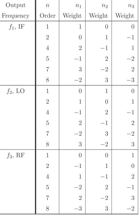
FREDA tabulated frequencies of interest in a table called the Basic Intermodulation Product Description (BIPD) Table [86]. A single entry in the table is referred to as a BIPD. Each BIPD is a set of integers that describes the weightings, nk of a set of K user-chosen frequencies, with each of the user-chosen frequencies having an integer, or tuple, assigned to describe the weighting, so that an output frequency fo is given by

fo n1f1 n2f2 . . . nkfk . . . fKnK . (2.1)