ABSTRACT
GHOSH, SHALINI. Framework to Quantify the Effects of Autonomous Vehicle Systems (Under the direction of Dr. Billy Williams).
The Highway Safety Manual (HSM)(AASHTO 2010) lays out a unified methodology to
calculate safety of a roadway segment or intersection based only on the physical features, design, and traffic volume of facility. To do so the HSM suggests different models based on the roadway facility type called, Safety Performance Functions (SPFs). In addition to SPFs, the HSM also suggests multiplicative factors for various treatments that might have been installed or are being considered for installation on the roadway facility called Crash Modification Factors (CMFs). The combination of the SPF and CMF estimates the average yearly number of expected crashes on specific roadway facilities. While new Autonomous assistance features are being installed in cars today, the HSM model framework does not include the effects of these features in the safety analysis.
This thesis suggests an extension and application of the HSM framework to model the effects of the autonomous features at a regional, statewide, or national network level. While the framework discussion assumes a statewide application and statewide application will likely be the most useful context, the framework can be applied at any level for which contemporaneous
autonomous vehicle market penetration rate and target crash data are available. The aim of this framework is to correlates the percent of target crashes a system reduces to its penetration rate. The data required to do so includes the total number of vehicles registered, the number of vehicles having the autonomous feature among the total vehicles registered, the total number of crashes in the state and their types and state-wide Vehicle miles Traveled (VMT). By using real data in this framework the effects for each assistive feature can be developed as a function of VMT and the penetration rate of the assistive system. These data could be obtained in part from insurance companies, Department of Motor Vehicles (DMV) and Insurance Institute for
Highway Safety (IIHS).
© Copyright 2019 by Shalini Ghosh
Framework for Developing Crash Modification Factors for Autonomous Vehicle Systems.
by Shalini Ghosh
A thesis submitted to the Graduate Faculty of North Carolina State University
in partial fulfillment of the requirements for the degree of
Master of Science
Civil Engineering
Raleigh, North Carolina 2019
APPROVED BY:
_______________________________ _______________________________ Dr. Billy Williams Dr. Nagui Rouphail
Committee Chair
ii DEDICATION
To Mom and Dad,
iii BIOGRAPHY
iv ACKNOWLEDGMENTS
It takes a lot of hard work to write a thesis. But, no matter how hard one works without mentors and contributors it is nearly impossible to realize an idea. For the fulfillment of this thesis, I would like to thank the following people.
Dr. Billy Williams, my advisor, professor, and mentor. It is difficult to find ideas. But it is even more difficult to curate that idea to make it productive. I am thankful to him, for having enough patience to curate my vague ideas and for his efforts to realize those ideas into this thesis. I also extend my gratitude towards Dr. Nagui Rouphail and Dr. Eleni Bardaka for their invaluable inputs to this thesis.
I thank Thomas Chase, my ex-supervisor at ITRE for making me the researcher I am today. I also thank him for helping me during some crucial analysis in this thesis.
I am thankful to Gregory Ferrara, ITRE for guiding me through the process of data collection which connected me to Brad Robinson and Shawn A. Troy at NCDOT. They were helpful enough to take time out and gather the data I needed from their system.
I would also like to thank, Prasad Bandodkar, for being my toughest critique throughout this thesis.
v TABLE OF CONTENTS
LIST OF TABLES ... vi
LIST OF FIGURES ... vii
1. INTRODUCTION ... 1
2. HSM METHOD FOR SAFETY ANALYSIS ... 3
2.1 Safety Performance Functions (SPF) ... 3
2.2. Crash Modification Factors (CMF) ... 3
2.3. Calibration of HSM ... 4
2.4. Developing new SPFs for North Carolina... 5
2.5. Developing location specific CMFs ... 5
3. AUTONOMOUS TECHNOLOGIES ... 7
3.1. Developments in AV technologies ... 8
Input Technologies... 8
Processing ... 10
Output ... 13
3.2. Impacts of AV on Safety ... 16
3.3. Dependency of System Effectiveness on its Market Penetration ... 18
4. FRAMEWORK ... 20
4.2. The Scope of the Model ... 20
4.3. Framework ... 21
Effects of Probable changes in Non-Vehicular Factors ... 21
Quantifying Effectiveness of AV systems ... 23
4.4. Applications ... 33
5. CONCLUSION ... 34
6. SCOPE FOR FUTURE RESEARCH... 35
7. REFERENCES ... 36
8. APPENDICES ... 41
8.1. Appendix A – HSM Calibration method... 42
vi LIST OF TABLES
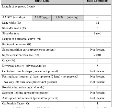
Table 1: Base Conditions for Rural 2 -Lane Undivided Road Segment ... 4
Table 2: Percent Reduction in Police report Crashes due to Lane Departure Warning System ... 14
Table 3: Percentage Reduction in Total crashes due to AEB, FCW, and combination of AEB&FCW ... 16
Table 4: Data for State-wide SPF development ... 27
Table 5: Vehicle registration Count ... 27
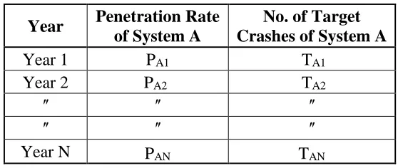
Table 6: Penetration Rate of System A ... 28
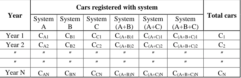
Table 7: Registration data for multiple systems ... 31
Table 8: Penetration Rate for Multiple systems... 31
Table 9: Parameter Estimates of new SPF developed for 2010 to 2015 data ... 44
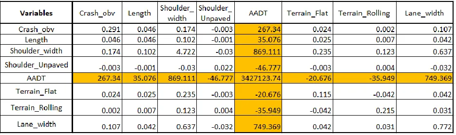
Table 10: Correlation Matrix of Variables in crash data ... 45
Table 11: Co-Variance Matrix of Variables in crash data ... 45
vii LIST OF FIGURES
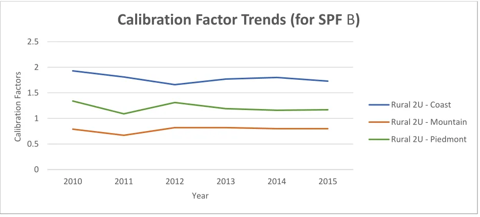
Figure 1: SAE Levels of Automation. Source: (SAE J3016 - Levels of Driving Automation 2019) ... 7 Figure 2: Framework Flowchart ... 23 Figure 3: Trend of Calibration Factors using SPF B (the HCM method) ... 46 Figure 4: Trend of Calibration Factors usin g SPF A (the SPF developed in
(Srinivasan and Carter 2010)) ... 47 Figure 5: Trend of Calibration Factors using SPF C (the new SPF developed-
table 9) ... 47 Figure 6: Trend of Calibration Factors using SPF D (the new SPF developed -
1 1. INTRODUCTION
The involvement of stochastic Human/Driver Behavior makes quantifying and forecasting traffic safety challenging. The Highway Safety Manual (HSM) (AASHTO 2010) establishes a
methodology to predict the safety of roadway and intersection sites based on site characteristics namely roadway features and design, and traffic volume. While Autonomous Vehicle (AV) are being designed to reduce and finally eliminate the human factor/behavior involved in driving, there is a lack of quantitative analysis to realize its effectiveness. This thesis sets a basic framework for achieving this goal.
The thesis starts by quantifying and predicting safety using HSM (AASHTO 2010) for the state of North Carolina. It then explores AV technologies that can affect safety in the future and finally suggests a framework to quantify the effect of these technologies on Safety. Previous research and predictions done by various researchers suggest that the number of crashes reduced due an AV technology depends on the number of vehicles equipped with that technology, but they do give a quantifiable correlation between them. Thus, the suggested framework uses Vehicle registration and Crash data of a state to correlate the penetration rate of an AV technology/system to its effectiveness on safety by extending the HSM (AASHTO 2010)
framework to a regional, statewide or national network level. Though this thesis focuses only on AV systems, this framework can be extended towards any vehicular features that have an effect on reducing collisions.
3 2. HSM METHOD FOR SAFETY ANALYSIS
The HSM (AASHTO 2010) lays out guidelines for screening hazardous sites, diagnosis of factors causing issues to safety, select countermeasures for improving safety, economic appraisals for implementing these countermeasures, prioritizing projects and evaluating the safety effectiveness. It provides performance functions and modification factors to predict the safety of a site even when actual observed data is not available.
2.2. Safety Performance Functions (SPF)
SPFs are equations used to predict the safety of a facility in terms of an average number of crashes per year, using its base/ untreated conditions. These SPFs were developed by fitting models to historical crash data assuming negative binomial distribution. The HSM (AASHTO 2010) provides a range of different SPFs for different types of sites. A list of base conditions is defined for each site type. Any characteristic of the site that deviates from the base conditions provided, needs an appropriate Crash Modification Factor (CMF) to be multiplied to the SPF for an accurate prediction.
Table 1 shows the base conditions for a Rural 2 lane Roadway as defined by the HSM (AASHTO 2010).
2.3. Crash Modification Factors (CMF)
Crash Modification Factors (CMF) are used to quantify the effects of road treatments and any other geometric or traffic feature that result in the study site characteristics to deviate from the base condition, on crash reduction. Like SPFs, CMFs provided in the HSM (AASHTO 2010) are also developed by fitting models to historical data. Every treatment has a different CMF
developed for it. The characteristic of the road that matches that of the given base conditions has a CMF value equal to 1.
4 2.4. Calibration of HSM
Calibration factors are the ratio of observed to the predicted number of crashes. Part C of the HSM (AASHTO 2010) desires a sample size of 100 crashes per year for a facility to be
calibrated. Calibrations have been done twice for the state of North Carolina by Srinivasan et al. in 2010 and Smith et al. in 2017 (Srinivasan & Carter, 2010; Smith, Carter, & Srinivasan, 2017). For detailed calibration method refer to Appendix A.
Table 1: Base Conditions for Rural 2-Lane Undivided Road Segment
Input Data Base Conditions
Length of segment, L (mi) --
AADT* (veh/day) AADTMAX = 17,800 (veh/day) --
Lane width (ft) 12
Shoulder width (ft) 6
Shoulder type Paved
Length of horizontal curve (mi) 0
Radius of curvature (ft) 0
Spiral transition curve (present/not present) Not Present
Super-elevation variance (ft/ft) < 0.01
Grade (%) 0
Driveway density (driveways/mile) 5
Centerline rumble strips (present/not present) Not Present Passing lanes [present (1 lane) /present (2 lane) / not present)] Not Present Two-way left-turn lane (present/not present) Not Present
Roadside hazard rating (1-7 scale) 3
Segment lighting (present/not present) Not Present Auto speed enforcement (present/not present) Not Present
Calibration Factor, Cr 1
5 2.5. Developing new SPFs for North Carolina
As mentioned already, SPFs and CMFs in the HSM (AASHTO 2010) are a result of model fitting on historical crash data. These historical data belong to a few cities from a select number of states. Though these are generalized equations and can be calibrated for any state, using local historical crash data to develop local SPFs and CMFs specific to a state would yield better predictions.
In addition to the calibration of HSM (AASHTO 2010), Srinivasan et al. also developed North Carolina (NC) Specific SPFs (Srinivasan and Carter 2010). The two types of SPFs that were tested were- 1)only considering AADT as the independent variable and Length of the segment as the weight variable and 2) considering - AADT/10000, ln(AADT/10000), Shoulder width, Shoulder type, terrain type as independent variables and segment lengths as the weight variable, out of which- terrain type and shoulder type were categorical.
Building on the efforts of Srinivasan et al., SPFs for Rural Two-Lane Undivided road segments were developed using recent data from NCDOT - SPF A. The calibration factor from SPF A was compared with the calibration factors from the SPF in HSM (AASHTO 2010) -SPF B and the one developed by Srinivasan et al. in 2010 - SPF C(Srinivasan and Carter 2010). SPF D was developed considering the statistical significance of variables and compared with the results from other SPFs. As anticipated the calibration factors calculated using SPF A, SPF C, and SPF D were closer to 1 as compared to calibration factors calculated using SPF B, indicating that the SPFs developed for NC with local data estimated crashes closer to what was actually observed. The calibration factors obtained from SPF A and SPF D were very close to each other implying that the statistical significance of variables had little effect on the performance of SPFs. Refer to Appendix B for detailed analysis and results.
2.6. Developing location specific CMFs
6 Research Safety Center n.d.) provides thousands of CMFs that are updated continuously based various researches from all over the United States and also internationally. But these CMFs account for the roadway features and traffic volume, but not for vehicle features.
Though, the development of state-specific CMF for various treatments was beyond the scope of this thesis the rest of the thesis is dedicated to understanding the importance of accounting for AV technology in safety calculation and suggesting a framework to develop a CMF for them.
7
3.
AUTONOMOUS TECHNOLOGIESA fully Autonomous Vehicle that can drive without the help of a human driver is the final and the highest level of Automation. There are some examples of driverless vehicles developed by different companies like Google (Waymo – Waymo n.d.), that are driven without human intervention only in specific locations and under specific conditions. Autonomous vehicles are not always equivalent to self-driving cars. There are 5 levels of autonomation as classified by Society of Automotive Engineers (SAE) (figure 1) (SAE J3016 - Levels of Driving Automation 2019):
Figure 1: SAE Levels of Automation. Source: (SAE J3016 - Levels of Driving Automation 2019)
8 As Özgüner et.al laid out in 2007, there are 3 necessary pieces of technology needs to perform perfectly for complete automation of vehicles (Özgüner, Stiller, and Redmill 2007):
1) Internal sensors like wheel and inertial sensors that stabilize the vehicle dynamics. This includes systems like Cruise Control, Anti-lock braking system, anti-skid control, etc. 2) Environmental sensors like sonar, radar lidar to gain information from the surrounding
environment that includes the road environment, vehicles, obstacles, etc. This is to provide assistance to human drivers.
3) Sensor Network like multi-sensor platform and distributed sensors to be able to control the longitudinal and latitudinal movement of the vehicle autonomously while avoiding collisions.
3.1. Developments in AV technologies
According to an American News and Opinion website (Plumer 2016), the major tasks that lay ahead for autonomous vehicles are the Understanding environment and human behavior to be able to interact in a mixed traffic situation consisting of vehicles ranging from Level 0 to Level 5 Automation. Continuous research is being done possible future technologies and algorithm that contributes to making the three functions of automation possible. Following are some examples of such efforts segregated in the three different functions: 1) Input, 2) Processing and 3) Output.
Input Technologies
Well-defined global mapping and GPS data are some common technologies used to position a vehicle. They are only capable of defining vehicle positions on a map but not capable of
centering a vehicle in a lane. Thus, as suggested by Wei et al. additional sensor for observing the environment are required to accurately position the vehicle on a roadway and to allow the
9 sensors are necessary (Özgüner, Stiller, and Redmill 2007). This section discusses the vision-based, Radar and Lidar-based systems in detail.
Vision-Based Systems
There are two categories of Monocular Vehicle Detection (Sivaraman and Trivedi 2013): i) Appearance-Based - used to detect the presence and the orientation of other vehicles
in the environment. Image recognition, computer vision, and machine learning are used for detection and classification of the captured image.
ii) Motion Based - differentiates vehicles from their background by their movements. This type of detection is used more commonly to detect overtaking vehicles
especially at the blind spot or to detect unusual maneuvering. It is less common for vehicle detection since it doesn’t give a 3D depth measurement.
The motion-based approach is more commonly used in AVs as compared to appearance-based approaches due to its ability to measure positions and velocities of other vehicles. Motion-based cameras are mounted on different sides on a single vehicle to verify images from all the cameras for accurate object classification.
Radar and LiDAR
• Radar sensors are used to detect the position and speed of objects directly, but they are not capable of classifying shapes (Wei et al. 2013).
• LIDAR uses the reflection of light photons to measure the shape and position of objects The data provided by LIDAR are a cloud of 3D points that are dense enough to know the shape of various vehicles and objects like cars, trucks, curbs, and pedestrian (Wei et al. 2013).
While LIDAR is stronger than radar in the field of object classification, Wei et al. point out its lower sensing range and its incompatibility with all weather conditions (Wei et al. 2013). However, LIDAR’s cost, sensing range, robustness to weather conditions and velocity
10 tandem and installed in the same position on a vehicle in order to utilize the strengths of each sensor
Processing
After inputs are gathered by different sources in the AV, it needs to process this information based on pre-designed algorithms to make the most accurate decision/output. Following are some of the algorithms for different functions that need to be performed by AVs.
Microscopic Scene Model
Microscopic scene models consist of three components; information measurement, information recognition, and information interaction as studied by (Gong et al. 2016). Data acquired by the sensors are collected in the Information measurement step. The information recognition step assesses all information measured by the sensor and sorts useful information for use in decision making, which is critical for estimating vehicle behavior. In the last step of information
interaction, the exchange of information between both vehicles and humans and vehicles and other systems, information is obtained through microscopic scene modeling. The information is used to find the probability of certain behaviors of other vehicles. One example is to determine the probability that a vehicle will yield. When tested, Microscopic scene modeling proved to be more reliable as compared to other modeling algorithms. Özgüner et al. too suggested that vehicular sensing should move from conventional sensing method to more consistent scene understanding for real trajectory planning (Özgüner, Stiller, and Redmill 2007).
Collision Avoidance Algorithms
A model for collision avoidance from an obstacle, based on the relative distance of the vehicle with the identified obstacles was designed by Durali et al., in 2006 (Durali, Javid, and
11 occupancy mapping method in which the shortest distance to an obstacle is calculated using sensors for avoiding a collision with obstacles (Özgüner, Stiller, and Redmill 2007). This model smoothens and re-plans the original trajectory in real time when the distance between the
obstacle and the vehicle is smaller than a predefined threshold.
In 2012 a model suggested by Shim et al. for collision avoidance used polynomial
parameterization method where the polynomial coefficients are determined by the boundary conditions and vehicles’ kinematics (Shim, Adireddy, and Yuan 2012). The algorithm is updated in real time, hence like the model designed by Durali et al. previously in 2006, this model could also be used for collision avoidance in case of both static and movable obstacles.
In a different framework suggested by Anderson et al. in 2011 trajectory planning was done through pre-planned corridors by assessing the threats and taking control actions using predictive and constraint handling mechanism for threat assessment, hazard avoidance, and path planning (Anderson et al. 2011). It assumes the existence of a path planner and image of the environment on a 2D map, on the basis of other literature that shows the feasibility of having such
information. The objective function is optimized in real time subject to certain constraints and input. The constraints include road boundary, speed, acceleration, etc. Slide slip angle of the vehicle was chosen as the objective function that needed to be reduced for the plan to be optimal since the side slip angle of the front wheel needs to be kept to a minimum to reduce the threat to vehicle stability and controllability.
Overtaking Maneuver
For Overtaking Maneuvers two mechanisms work simultaneously (Naranjo et al. 2008). These two mechanisms can be broadly classified as lane keeping and lane changing mechanisms. The first step of the process is changing to the left lane and to stay in that lane until the vehicle to be overtaken is passed. The second step is returning to the original lane and then switching back to the lane keeping mechanism. In all the steps the vehicle’s speed and steering need to be
controlled. Gong et al. identified 5 sub-states within these two mechanisms for legal overtaking maneuvers (overtaking from the left), namely (Gong et al. 2016):
12 2) Lane changing to the left lane (LC2L);
3) Overtaking (Passing);
4) Lane change preparing to the right lane (LCP2R); 5) Lane changing to the right lane (LC2R).
Moving into details about the overtaking maneuvers Gong et al. specifies that the state for overtaking can be reached only from a state of lane keeping (Gong et al. 2016). This transition can be caused by both intention (driver preference) or relevant condition (safety, comfort, a possibility of overtaking, etc.). After determining the intention for transition the benefits and cost of overtaking functions are determined. If the benefit is a certain percentage more than the cost, then the vehicle transitions from the state of “Lane Keep” to “Overtake”. Similarly, for the transition from LCP2L to passing, the benefit function needs to be a certain percentage more than the cost, which depends on the probability of overtaken vehicle to yield. The automated vehicle (overtaking vehicle) overtakes the slow-moving vehicle without slowing down. The stabilization system makes sure that the steering angle is within a stable steering range.
Human-Like Decision Making
Li et al. focused on building a making system that could imitate humanlike decision-making skills (Li, Ota, and Dong 2018). This model is particularly important during the
transition phase from conventional vehicles to 100 % self-driving vehicles in the traffic stream, when roads will be shared by different level of AVs. This suggested method consists of 4 main steps (Li, Ota, and Dong 2018):
1) Input: for data collection, which in case of the research done by Li et al. are images of the scene/environment in which the vehicle is being driven
2) Abstraction: to simplify the data input for the system to understand better.
3) Decision Making: to make necessary decisions for the vehicle, based on set algorithms using the data abstracted.
13 Decision-Making Network (DMN) is taught to make human-like decisions by feeding the
algorithm with previous data of different scenarios and the decisions made by humans in them. Hence, based on historical data the DMN would replicate human decision-making ability for a new situation the vehicle faces. Along with the DMN, a safety enforcement method is added to rectify the decisions that cause risk to safety. This secondary mechanism is what forces the vehicle to follow traffic regulations and keep lanes. The study’s tests results show that vehicles in this model drove slower than human drivers due to extra safety enforcement. It is also inferior to human drivers due to the absence of social intelligence possessed by human drivers.
Output
The final aim of the AVs is to be able to process inputs and make decisions for the action it needs to take, which ranges from assisting the driver to perform a specific function to make all the decisions required to drive itself without any human intervention (Automation Level 0 to 5). At Automation Level 0 output can be seen as guidance or warnings for the driver to prevent risks to safety, but its benefits totally depend on the final action driver decides to take (Winkler, Kazazi, and Vollrath 2018). As Levels of Automation increase, outputs become actions take the form of assistance to the driver. At Levels 1 and 2 the actions taken by the system could be overridden by the human driver, but at higher Automation levels as systems become more reliable the control shifts from the driver to the system.
The autonomous technologies used currently are more towards assisting drivers to improve safety and quality of driving (level 0 to level 2) (Özgüner, Stiller, and Redmill 2007). Due to uncertainties associated with these sensors till date, even after the vehicles take decisions to assist the driver, the final decision to whether or not comply with the system remains with the human driver.
14 Lane Departure Warning (LDW) and Lane Departure Prevention (LDP)
LDW and LDP both aim at assisting the driver in lane keeping. In case of LDW when the system notices an unintentional drift from the lane (drifting to another lane without an indicator) it warns the driver using an audible or visual aid. But in case of LDP instead of a warning, the system corrects the steering, braking or accelerating one or more wheels or any combination of them to return the vehicle to its original lane.
The Insurance Institute for Highway Safety (IIHS) report shows the effect of LDW systems on relevant crashes i.e single vehicle sideswipe and head-on crashes as presented in table 2. The analysis was done twice- Once without controlling for driver demographic factors and second after controlling for driver demographic factors. The driver demographic factors considered were - driver age, gender, insurance risk level and other factors that could affect the rates of crashes per insured vehicle year.
Table 2: Percent Reduction in Police report Crashes due to Lane Departure Warning System
Without Controlling for Demographic Factors
After Controlling for Demographic Factors All relevant Crashes
(in %) 18 11
Injury Crashes (in %) 24 21
Fatal Crashes (in %) 86 0
Source: (IIHS 2017)
15 Forward Collision Warning (FCW) & Automatic Emergency Braking (AEB)
FCW and AEB both aim to prevent the vehicle from striking the rear end of the vehicle in front of it when the system recognizes that the relative speed of the two vehicles can cause a crash at the distance between the two vehicles. FCW warns the driver of the possibility of such collision and the driver is expected to take actions based on this warning. There are still some limitations of such systems. Yue et al.. points out in his research that adverse weather conditions hamper the functioning of these systems, like fog in case of FCW.
In 2016, Cicchino evaluated the effectiveness of FCW with and without AEB in crash reduction (Cicchino 2016). They use police reported crashes as the study data for this. Through regression analysis of the data and controlling for covariates, it was found that FCW alone was associated with a reduction of 23% of rear-end striking crash rates and FCW with AEB was associated with a reduction of 39% for the same. A later evaluation by Cicchino using crash data from police reports, the exposure (i.e the number of days the vehicle has been insured) from insurance records compared the crash involvement rate per insured vehicle year using Poisson regression model (Cicchino 2017). Vehicle models having FCW and AEB as optional features were used for the comparison to compare similar models having only FCW, only AEB, and both FCW and AEB. Three crash types were involved in the study – 1) rear end striking crashes, 2) rear end striking crashes with injuries, 3) rear end striking crashes with third-party injuries. A logarithmic model was used to compare the crash involvement rate ratio of vehicles with - 1) FCW to
vehicles that are not equipped and 2) with FCW and AEB to vehicles that are not equipped. After controlling for state, calendar year, registered vehicle density of the vehicle garaging location, collision coverage deductible range, and the age, gender, marital status, and insurance risk of the rated driver, the analysis showed that FCW alone was associated with a 27% reduction in rear-end striking crash rates, low-speed AEB was associated with a 43% reduction and FCW with AEB was associated with 50% reduction.
16 In the same research, Cicchino also found that the rear end struck rates (the rate of the study vehicle being rear-ended) were 20% higher in case of vehicles with FCW and AEB than vehicles without any systems (Cicchino 2017).
Table 3: Percentage Reduction in Total crashes due to AEB, FCW, and combination of AEB&FCW
System Used
Reduction in Total crashes (%)
FCW 6.3
AEB 10.1
FCW+AEB 11.7
In the next year research carried out by Yue et al., warning messages were given to the driver when the headway between it and the vehicle in front was less than 400ft. On comparing the effectiveness of vehicles having such systems to vehicles that don’t, based on the proportion of vehicles in near-crash events it was found that the decrease in the proportion of near-crash events without FCW to FCW) was 0.35 (35%). Near crash events, in this case, were defined when vehicles’ Time-to-Collision (TTC) was lesser than the threshold TTC (of 2 seconds) (Yue et al. 2018).
3.2. Impacts of AV on Safety
17 Madigan et.al simulated manual and automated driving situations using a driving simulator and found even though the automated trajectory was different from the ones followed by the
participants during manual driving, they preferred automated driving over manual driving and systems where the driver needs to intervene (Madigan, Louw, and Merat 2018). Even though the crash rates might decrease Fagnant and Kockelman forecast that there would be more pent up demand in the early adopters in comparison with the late buyers, which will increase the total vehicle miles traveled leading to a net increase in crash and injury (Fagnant and Kockelman 2015b).
Schoettle et al. discovered a very peculiar crash behavior of AVs from the crashes reported by the self-driving fleet operated by Google, Audi, and Delphi. It found that the majority of crashes involving AVs occurred when they were stationary or moving very slowly (<= 5mph) and all the crashes involved another motor vehicle. Self-driving cars were rear-ended 1.5 times compared to conventional cars whereas they were not involved in any head-on collisions (Schoettle and Sivak 2015). This implied that in all the crashes involving the Self-driving cars with a conventional motor vehicle, the latter was at fault. In spite of impressive outcomes, the study lacked validation since data for self-driving cars were limited as a result of only being driven in certain limited conditions and not statistically comparable to the millions of miles traveled by conventional cars. Safety of AV as pointed out by Litman in 2018 is also dependent on the amount of risk the
vehicle is programmed to take to maintain a trade-off between how fast the vehicle can operate to increase road capacity and the margin of safety it operates with (Litman 2018). There are newly added risks to safety with the new technology like system failure, delay in
18 3.3. Dependency of System Effectiveness on its Market Penetration
Most studies calculating the effectiveness of an assistance feature overlook the market penetration rate of the feature. Their results are based on the assumption that all vehicles are equipped with assistive systems (i.e 100% penetration rate of assistive systems). But, as shown in the following sections, the effectiveness of the system to reduce crashes increases with market penetration of a system.
Increase in market penetration is a gradual, uneven process. Specifically, the in-car advisory system’s performance is dependent on the compliance rate of the drivers. Risto et al. found that an individual driver’s compliance with the system is based on the compliance rate of other drivers in the traffic stream (Risto and Martens 2014). In this study, the drivers’ behavior was judged using a driving simulator, based on the actual compliance rate of the traffic stream and the compliance rate of the traffic stream as perceived by the driver. Vehicles equipped with the advice algorithm showed different behavior as compared to conventional vehicles. The study concluded that drivers were less likely to continue complying to the system if they do not find a direct advantage. When the drivers got more information from the advisory system, their
expectation from other drivers increased and the compliance rate perceived by them was an underestimation of the actual compliance rate. Thus, the driver ceased to comply with the system henceforth. In contrast, uninformed drivers overestimated the compliance rates of the traffic stream and proved to be are more likely to comply with the system.
A study done on Adaptive Cruise Control (ACC) systems by Mardsen et al. showed that the average journey time increased with increasing penetration rates of ACC especially at the highest demand due to greater target time gap for of the system safety measures as compared to the relatively unsafe time gaps preferred by drivers during rush hours (Marsden et al. 2000). The system studied operated above a certain speed and gave the driver full control to over-ride its decisions any time. This research assumed that the system was used whenever it could be
19 traffic since heavy vehicle drivers are already more cautious. Along with these conclusions, platoon instability was also observed due to significant deceleration when the driver resumes control from the ACC system.
In 2017, Cicchino that found that vehicles with FCW and AEB had lesser chances of rear-ending a vehicle in front of it compared to vehicles without any systems also found that the same vehicle had 20% more chances of being rear-ended as compared to a vehicle without any system
(Cicchino 2017). This was a result of sudden braking either by AEB or by the driver in response to FCW. This gives a picture of how the adoption/penetration rate of a system plays a big role in its effectiveness in reducing crashes as a whole. If the vehicle following the subject vehicle also had FCW and AEB then rear-end collisions can be prevented. Thus, extrapolating this effect if every following vehicle had FCW and AEB there would be no rear-end collisions.
20
4.
FRAMEWORKTo account for the effects of an AV system on the number of crashes historical data is required. Since AV systems are relatively new, not a lot of historical data is available and hence, these models need to be updated as and when new data is available. It needs to be kept in mind that the effectiveness of an assistive system will differ with the percentage of vehicles equipped with that system in the traffic stream. This Framework is developed by closely following the steps used for developing SPFs and CMFs in the HSM. But, unlike the SPFs and CMFs suggested by the HSM, the framework builds a model that is at a state wide level
The penetration rate of a system A is defined as the ratio of the number of cars having system A to the total number of cars, in a state. Since cars are not specific to a particular area, the effects of systems in cars need to be modeled as a state-wide effect. Along with the changes in penetration rates of the system, other non-vehicular factors change over the years and have a role to play in safety. For example, even if the systems are effective enough in reducing the rate of crashes, there might be an increase in Vehicle Miles Travelled (VMT) that will lead to more number of crashes overall as predicted by Fagnant and Kockelman (Fagnant and Kockelman 2015b). Thus, the framework also suggests and describes the procedure to develop a state-wide SPF based on the state-wide VMT. It also includes ways to include changes that affect safety other than vehicular systems and VMT.
“Vehicles” in this thesis henceforth mean, light duty personal/ commercial vehicles (which include Sedan, SUV, hatchbacks).
4.2. The Scope of the Model
CMF, as defined by FHWA is a measure of safety effectiveness of a treatment or design element. It is a multiplicative factor that gives the proportion of crashes to be expected after the
installation of treatment or countermeasure (FHWA n.d.). The CMFs in HSM and CMF
21 94% of crashes as calculated by the National Highway Traffic Safety Association (NHTSA), the AV technologies that help drivers during driving and gradually eliminate the need for humans to drive, are going to have a major effect on safety, that are not accounted by CMFs (Highway Traffic Safety Administration and Department of Transportation 2015). Thus, while preparing roads for an Autonomous future, safety prediction and evaluation methods also need to be updated. The model framework suggested in this thesis is a foundation towards achieving that goal.
The model framework suggested here can be put to use by following the steps listed in the following sections. The type of data required for this model can be found in Insurance records and crash reports. But they are not available publicly due to the privacy and confidentiality related to them. Researchers can request these data as an aggregate from certain institutes, without revealing the identity of any individual vehicle or compromise their privacy in any way. But, this kind of data was not available for this thesis Thus, it only suggests the framework. Though, there are researches that quantify the effects of a system by calculating the reduction in crashes caused by them, they only focus on one system. But, this framework includes all factors affecting a type of crash for an accurate unbiased estimation.
4.3. Framework
The framework is divided into 2 parts. The first one is detail description of possible factors affecting safety in a short period of time, the second part is a methodology to derive a function to quantify the effects of penetration rates of assistive systems along with an SPF as a function of VMT.
Effects of Probable changes in Non-Vehicular Factors
22 good way to analyze these factors (Hauer 2015). The following are some of the major factors that should be kept in mind.
Demographic Changes of Drivers
As we move towards a more Autonomous Future, the task of driving will move away from humans to the vehicle itself. Thus, types of trips, number of trips and trip length may change but the type of occupants or drivers will not be playing a role in the driving activity or influence road safety.
Policy Changes
Along with the introduction of new technologies, policies related to transportation are likely to change. Though these changes take time to be implemented they occur relatively within a short period of time than factors like population, demographics, etc. that change over a long period of time. Thus, in case of drastic policy changes, it is best to compare the crash data before and after the policy was implemented. Any drastic change in a number of crashes between the before and after period could be attributed to this policy change. The crashes should be segregated and compared by their types. For example, the changes in Rear- end and sideswipe crashes should be calculated separately.
Land Use Changes
Land Use change slowly with the development of a state’s economy and preferences. In the future, there is a possibility of land use changes due to the introduction of AVs due to the change in trip patterns and durations. But, this change would be gradual since it is not practical to
23 Infrastructural Changes
AVs might require some notable changes and improvements in the road infrastructure. These changes and improvements apart from being required for AVs can also help drivers. At the same time, there can be a negative effect as well. Thus, the effect of these infrastructures on human drivers and in turn their effects on safety need to be isolated. To do so, for each type of crashes, two types of vehicles need to be considered. The first type would be vehicles having a system that had systems that could prevent that type of crash, and the second category would be vehicles that did not have a system related to it. For example, to study the effects of the infrastructure on Rear- End Collision, cars having systems like FCW and AEB need to be separated from cars having no systems to prevent a rear-end collision. The crash behavior of the latter group of vehicles should be studied to compare their crash rates before and after the change in infrastructure to understand the changes in crashes due to the infrastructure.
Quantifying Effectiveness of AV systems
The SPF models used at present are road or intersection specific. But, since the effect of AV systems are to be studied statewide it cannot be used with the existing SPF models suggested by the HSM to avoid any biased estimation for a specific roadway. The step-wise procedure to develop a function to quantify the effectiveness of AV systems described in the following sections. Figure 2 gives a flowchart of the entire procedure at a glance.
Figure 2: Framework Flowchart
Data collection Data analysis Quantifying effects Final Model
1. VMT of state
2. Number of
Vehicles Registered in a year and
systems installed in them.
3. Annual state
wide crashes and their types.
1. VMT vs. target crashes
2. Penetration
Rate of System
1. Expected Crashes
as a function of VMT
2. Quantifying the
effects of AV systems on target crashes in addition to VMT
E(Crash A) =
𝑓(𝑉𝑀𝑇) × 𝑓(𝑃𝐴)
where,
f(VMT) – function of VMT
f(PA) – function of
24 Step 1 – Data Collection
It is better to collect data beginning from a time when the AV systems were not introduced in any vehicles. This gives a better preview of how the number of crashes varied with varying VMT without the presence or effect of any AV systems. But, in case data from such a time is not available, it is okay to begin the data collection from a date after the systems were introduced into vehicles. The details of the data to be collected to model the effects of an AV system A, are as follows:
1) The number of years of data to be collected. The framework can be implemented with a few years of data but in regression it is always advisable to have more data points. Thus, it is encouraged to collect data for at least 15 or more number of years. These years can be consecutive but that is not a necessity. These years just need to be arranged in ascending order.
2) The state wide VMT of every year, and the number and type of crashes in a year in a state need to be collected.
3) We need to collect the number of cars registered and the number of cars having assistive system A installed in them for each year. If the data set spans from a time where AV system was not available, then the number of cars with system A installed in it were 0. Thus, for those years we only need to collect the total number of vehicles registered in the state.
4) After information on vehicles we need to collect data for the number and types of crashes that occurred in the state for every year in our data set. These type of crashes should be segregated by target crashes of the system to be modelled. The following section (section 4.2.2.2) explains target crashes and lists the target crashes of some widely used AV systems.
Assistive Systems and their target crashes
25 i) Forward Collision Warning –
It is a system that warns the driver of an impending crash in case it gets too close to the car in front of it by monitoring relative speed and distance between the two cars.
Target Crash: Rear end crashes. (Driver Assistance Technologies | NHTSA n.d.)
ii) Automatic Emergency Braking Systems
1) Dynamic Brake Support (DBS):
DBS acts to enhance the driver’s braking when it thinks that the driver did not brake hard enough to avoid rear-ending the vehicle in front of it.
Target crash: Rear end crashes. (Driver Assistance Technologies | NHTSA n.d.)
2) Crash Imminent Braking (CIB)
CIB kicks in to avoid a collision when it senses that the driver is not braking to do so. Target crash: Rear end crashes (Driver Assistance Technologies | NHTSA n.d.)
iii) Pedestrian Automatic Emergency Braking (PAEB):
PAEB automatically breaks the car when the system senses a probable collision with the pedestrians in front of the vehicle and the driver does not break to avoid the crash.
Target Crashes:
a) Crashing into a pedestrian crossing the road;
b) Crashing into a pedestrian walking along or against traffic. (Driver Assistance Technologies | NHTSA n.d.)
iv) Blind Spot Monitor Warning
26 Target Crashes: Crashes caused due to the subject vehicle merging or changing lanes. (Cicchino 2018)
v) Lane Departure Warning (LDW)
It is a warning system to alert the driver of unintentional drift from its lane without a turn signal.
Target Crashes:
a) Sideswipe crashes b) Head on collisions
c) Rollover crash, due to the vehicle leaving the road. (Driver Assistance Technologies | NHTSA n.d.)
vi) LDP / Lane Keep Assist (LKA)
The LKA like LDP also activates when it thinks that the car is drifting unintentionally from its lane.
Target Crashes:
a) Sideswipe crashes b) Head on collisions
c) Rollover crash, due to the vehicle leaving the road. (Driver Assistance Technologies | NHTSA n.d.)
After segregation of crash data according to target crashes of the system, basic analysis needs to be performed on them to arrange them in the way needed to finally derive a model from it.
Step 2 - Data Analysis
27 1) The VMT for each year and the number of target crashes of each year in our data set
needs to be arranged in the manner shown in Table 4, where Viis the state wide VMT in
year i and Tjiis the number of target crashes of system j in year i in the entire state.
Table 4: Data for State-wide SPF development
Years State-wide VMT
No of Target Crashes of
System A
Year 1 V1 TA1
Year 2 V2 TA2
ʺ ʺ ʺ
ʺ ʺ ʺ
Year N VN TAN
2) The next step of the data analysis is to calculate the penetration rate of System A for every year. Penetration rate is the percent of vehicles equipped with system A in the total number of vehicles registered in a year. For that we first need to bring data related to vehicles registered in the form shown in Table 5, where Cji is the number of cars registered in year i equipped with system j and Ci is the total number of vehicles registered in year i.
Table 5: Vehicle registration Count
Year Cars registered with System A
Total Cars Registered
Year 1 CA1 C1
Year 2 CA2 C2
ʺ ʺ ʺ
ʺ ʺ ʺ
Year N CAN CN
Thus, penetration rate will be calculated as the ratio of cars registered with system A in a year to the total number of cars registered in that year. That is the penetration rate of system A in year M of is = 𝐶𝐴𝑀
𝐶𝑀. Thus, the penetration rate of system A for each year
28 where Pji is the penetration rate of system j in year i and Tji is the number of state wide
target crashes of system j in year i.
Table 6: Penetration Rate of System A
Year Penetration Rate of System A
No. of Target Crashes of System A
Year 1 PA1 TA1
Year 2 PA2 TA2
ʺ ʺ ʺ
ʺ ʺ ʺ
Year N PAN TAN
Step 3 – Quantifying effects of variables
The first step to start building the model is to fit a model in the values given in Table 4. By fitting a model in that data, we will get the expected number of target crashes of System A across the state as a function of VMT of the state. This function is like an SPF since it takes a basic variable to estimate the number of a type of crash. It is best to plot the number of Target crashes of system A vs VMT to understand the type of model that needs to be fit in it. If the data set has data from the time when system A was not introduced to any vehicles, then the trend of crashes in this graph for those years are expected to be smooth, unless there are any other factors like the ones mentioned in section 4.2.1. But for the trend of target crashes after system A was
introduced this graph is supposed to deviate from the trend it was previously showing. This means that there are other factors that are affecting the number of crashes other than the VMT. The function obtained from this step will look like the following:
E(Crash A) = 𝑓(𝑉𝑀𝑇)
--- Equation 1: Estimated crashes as a function of VMT only Where,
29 f(VMT) – Function of VMT. The type of function depends on the type of model fitted during
regression of data from Table 6.
For example, if after studying curve of number of target crashes vs. VMT, the analyst decides to fit a logarithmic model, then Equation 1 will become:
E(Crash A) = 𝛼 + 𝛽0𝑒𝛽1×𝑉𝑀𝑇
--- Equation 2: Exponential model fit Where,
Variables are as defined for Equation 1
β0, β1 are parameters fitted using regression analysis to minimize the error of the observed to the
estimated number of crashes
Now, taking inspiration from exploratory data analysis suggested by Hauer, the other variables that affect the function need to be explored and quantified (Hauer 2015). The other variable in this case is penetration rate of the system. While applying this model the analyst might find other variables that they think could have a significant effect on the expected number of crashes. In that case those variables and their effects need to be quantified using the same method.
To include the effect of penetration rate on the number of target crashes in addition to the VMT, the equation will become as follows:
E(Crash A) = 𝑓(𝑉𝑀𝑇) × 𝑓(𝑃𝐴)
--- Equation 3: Combined effect of VMT and penetration rate Where,
Variables are as defined for Equation 1
f (PA) - function of penetration rate of system A
30 penetration rate of System A is zero. It is also expected that crashes reduce with increasing penetration rate of a system, thus 𝑓(𝑃𝐴) should . For example, if from the graph plotted if the analyst feels that the relation between target crashes and penetration rate is exponential, the function of penetration rate in equation 3 would be of the form:
𝑓(𝑃𝐴) = (1 − 𝛽2𝑃𝐴𝛽3)
--- Equation 4: Function of Penetration Rate Where,
Variables are as defined in equation 3. β2, β3 – fitted parameters
PA ϵ [0,1]
𝑓(𝑃𝐴) can be viewed as Crash modification factor for system A because it is an added specific factor that modifies the general equation that uses VMT to estimate the number of target crashes. Equation 2 and Equation 4 needs to be then combined for the final model for estimating the expected number of target crashes of system A.
E(Crash A) = (β0eβ1×VMT) × (1 − 𝛽
2𝑃𝐴 𝛽3)
---- Equation 5: Final equation for combined effect
Though, some of the parameters were estimated for Equation 2, the parameters need to be estimated again considering Equation 5 as the model to be fitted into the observed data. The mean squared error needs to be minimized to estimate the parameter values of β0, β1, β3.
The final step is to make sure if there are any more unexplained differences between the
31 Target Crashes Common to multiple systems
There are some similar AV systems that target the same type of crashes. Thus, the change in the number of target crashes will depend on the effects of all the similar systems. For example, FCW and AEB both target rear-end crashes. The method to develop Equation 1 are the same as
explained in the previous section. But instead of only considering vehicles equipped with system A in this case there are vehicles that are equipped with one or more than one system having the same target crashes. Thus, along with vehicles segregated according the individual systems installed in them, they also need to be categorized by the combination of features they have. For example, if system A, B and C have the same type of target crashes, then vehicle with system A, system B, system A+B, System A+C need to be categorized separately. Thus Table 5 in this case will be modified to Table 7. Similarly, Table 6 will be modified to Table 8.
Table 7: Registration data for multiple systems
Year
Cars registered with system
Total cars System A System B System C System (A+B) System (A+C) System (A+B+C)
Year 1 CA1 CB1 CC1 C(A+B)1 C(A+C)1 C(A+B+C)1 C1
Year 2 CA2 CB2 CC2 C(A+B)2 C(A+C)2 C(A+B+C)2 C2
ʺ ʺ ʺ ʺ ʺ ʺ ʺ ʺ
ʺ ʺ ʺ ʺ ʺ ʺ ʺ ʺ
Year N CAN CBN CCN C(A+B)N C(A+C)N C(A+B+C)N CN
Table 8: Penetration Rate for Multiple systems
Year
Penetration Rate of system No. of
Target Crashes System A System B System C System (A+B) System (A+C) System (A+B+C)
Year 1 PA1 PB1 PC1 P(A+B)1 P(A+C)1 P(A+B+C)1 TA1
Year 2 PA2 PB2 PC2 P(A+B)2 P(A+C)2 P(A+B+C)2 TA2
ʺ ʺ ʺ ʺ ʺ ʺ ʺ ʺ
ʺ ʺ ʺ ʺ ʺ ʺ ʺ ʺ
32 The effect of VMT on the target crash will still be defined by the model given in Equation 1. But, now, since there are multiple systems whose effects need to be quantified the correlation of these systems with each other needs to be calculated to make sure that the model would not over represent or under represent a system. For example, if it was found that system (A+B) and system (A+C) are correlated then, the analyst needs to choose either one of them depending on which variable reduces the amount of error in the model. To make that decision the analyst will need to do multiple regression trials with the different possible sets of variables. In the above example where system (A+C) and system (A+B), the Equation 3 will be modified to either of the following (Equation 7a or Equation 7b) depending on which model gives a better fit.
E(Target Crash) = 𝑓(𝑉𝑀𝑇) × 𝑓(𝑃𝐴) × 𝑓(𝑃𝐵) × 𝑓(𝑃𝐶) × 𝑓(𝑃𝐴+𝐵) × 𝑓(𝑃𝐴+𝐵+𝐶)
--- Equation 6a: Combined equation for multiple systems (Case 1)
E(Target Crash) = 𝑓(𝑉𝑀𝑇) × 𝑓(𝑃𝐴) × 𝑓(𝑃𝐵) × 𝑓(𝑃𝐶) × 𝑓(𝑃𝐴+𝐶) × 𝑓(𝑃𝐴+𝐵+𝐶)
--- Equation 7b: Combined equation for multiple systems (Case 2)
Where,
E(Target Crash) – Expected number of Target Crashes of System A,B and C
f(VMT) – Function of VMT developed to quantify the effects of VMT on number of target
crashes of Systems A, B and C.
f(Pi) – function of penetration rate of system i
i – A, B, C, A+B, A+C, A+B+C
To calculate the exact function of penetration rate of all the individual and combination of systems, first a graphs for the penetration rate of each of the systems and combinations
33 4.4. Applications
34
5.
CONCLUSIONIn this thesis, a framework is suggested as an extension of the HSM framework at a state-wide level to develop a model for quantifying the effects of an AV system on safety. The penetration rate is one of the important factors in judging the performance of an AV system. With an
increase in the market share of a system, its effectiveness increases, and crashes are expected to reduce. Hence the model framework suggested uses the penetration rates of a system to model its effectiveness in reducing crashes. Since the effect of the AV system is quantified at a state-wide data level, a model to correlate state VMT with expected number of crashes of using it along with an SPF based on statewide data rather than individual road type data would yield more accurate results. Thus, this framework also suggests the derivation of a state-wide SPF based on Vehicle Miles Travelled in the state.
Thus, it can be concluded that the framework suggested in this thesis could be used as a starting point for estimating the effect of assistive systems in vehicles as a part of safety analysis since this framework considers all factors affecting crashes for an unbiased and accurate judgement. The CMF developed using this framework can also serve as an indicator of how effective a system is, and whether it is beneficial or not. As gradual progress is made with assistive systems and it finally evolves into a driverless future, there will be a requirement for models to judge safety only based on vehicle systems. The analysis for safety needs to evolve keeping that in mind.
35
6.
SCOPE FOR FUTURE RESEARCHWhile scanning through the literature related to Autonomous vehicles and future predictions and plans related to them, there were a few gaps that were noticed. But, due to the limited scope of the project and the timeline, these research scopes could not be explored for this project. Thus, the following are some suggestions that could be worked on in future research
1) Though the crash rate is predicted to decrease with the level of automation, (Fagnant and Kockelman 2015a) suggests the total number of crashes may increase since the number of miles traveled will increase due to the ease of mobility. Concerns related to safety are higher in the transition stages when Self-driving vehicles share the road space with human-driven vehicles due to the fundamental difference in their method of operation. More research effort needs to focus on this transition phase. Simulation models for different traffic compositions with vehicles ranging from Level 0 to Level 5 Autonomous Technologies should be tested.
2) Since V2V and V2I technologies for vehicles are evolving, we need a framework to quantify the effectiveness of these systems.
36
7.
REFERENCESAASHTO. 2010. Highway Safety Manual. 1st ed. American Association of State Highway and Transportation Officials (AASHTO).
https://app.knovel.com/web/toc.v/cid:kpHSM00002/viewerType:toc//root_slug:highway-safety-manual (March 11, 2019).
Anderson, Sterling J., Steven C. Peters, Tom E. Pilutti, and Karl Iagnemma. 2011. “Design and Development of an Optimal-Control-Based Framework for Trajectory Planning, Threat Assessment, and Semi-Autonomous Control of Passenger Vehicles in Hazard Avoidance Scenarios.” In Springer, Berlin, Heidelberg, 39–54. http://link.springer.com/10.1007/978-3-642-19457-3_3 (August 31, 2018).
Cicchino, Jessica B. 2017. “Effectiveness of Forward Collision Warning and Autonomous Emergency Braking Systems in Reducing Front-to-Rear Crash Rates.” Accident Analysis & Prevention 99: 142–52.
https://www.sciencedirect.com/science/article/pii/S0001457516304006 (January 18, 2019). Cicchino, Jessica B. 2016. Effectiveness of Forward Collision Warning Systems with and without
Autonomous Emergency Braking in Reducing Police-Reported Crash Rates.
https://orfe.princeton.edu/~alaink/SmartDrivingCars/Papers/IIHS-CicchinoEffectivenessOfCWS-Jan2016.pdf (January 18, 2019).
———. 2018. “Effects of Blind Spot Monitoring Systems on Police-Reported Lane-Change Crashes.” Traffic Injury Prevention.
http://www.tandfonline.com/action/journalInformation?journalCode=gcpi20 (January 22, 2019).
“Driver Assistance Technologies | NHTSA.” USDOT. https://www.nhtsa.gov/equipment/driver-assistance-technologies (January 18, 2019).
37 Fagnant, Daniel J., and Kara Kockelman. 2015a. “Preparing a Nation for Autonomous Vehicles:
Opportunities, Barriers and Policy Recommendations.” Transportation Research Part A: Policy and Practice 77: 167–81.
https://www.sciencedirect.com/science/article/pii/S0965856415000804 (September 17, 2018).
———. 2015b. “Preparing a Nation for Autonomous Vehicles: Opportunities, Barriers and Policy Recommendations.” Transportation Research Part A: Policy and Practice.
FHWA. KABCO Injury Classification Scale and Definitions.
https://safety.fhwa.dot.gov/hsip/spm/conversion_tbl/pdfs/kabco_ctable_by_state.pdf (March 16, 2019).
Gong, Jianwei, Youzhi Xu, Chao Lu, and Guangming Xiong. 2016. “Decision-Making Model of Overtaking Behavior for Automated Driving on Freeways.” In 2016 IEEE International Conference on Vehicular Electronics and Safety (ICVES), IEEE, 1–6.
http://ieeexplore.ieee.org/document/7548162/ (September 4, 2018).
Hauer, Ezra. 2015. “Exploratory Data Analysis.” In The Art of Regression Modeling in Road Safety, Cham: Springer International Publishing, 29–45.
http://link.springer.com/10.1007/978-3-319-12529-9_3 (April 25, 2019).
Highway Traffic Safety Administration, National, and Us Department of Transportation. 2015. TRAFFIC SAFETY FACTS Crash • Stats Critical Reasons for Crashes Investigated in the
National Motor Vehicle Crash Causation Survey.
https://crashstats.nhtsa.dot.gov/Api/Public/ViewPublication/812115 (February 27, 2019). IIHS. 2017. Insurance Institute for Highway Safety | Highway Loss Data Institute Status Report
Vol. 52, No.6.
https://www.iihs.org/iihs/news/desktopnews/stay-within-the-lines-lane-departure-warning-blind-spot-detection-help-drivers-avoid-trouble (January 18, 2019). Knipling R, Ronald (NHTSA);, Inc.) Wang, Jing-Shiarn (IMC, and Inc.) Yin, Hsiao-Ming (IMC.
1993. “Rear-End Crashes: Problem Size Assessment And Statistical Description.” https://rosap.ntl.bts.gov/view/dot/2902 (January 23, 2019).
Decision-38 Making System for Autonomous Vehicles.” IEEE Transactions on Vehicular Technology 67(8): 6814–23. https://ieeexplore.ieee.org/document/8330044/ (September 8, 2018). Litman, Todd Alexander. 2018. Autonomous Vehicle Implementation Predictions Implications
for Transport Planning. [email protected] (August 31, 2018).
Madigan, Ruth, Tyron Louw, and Natasha Merat. 2018. “The Effect of Varying Levels of Vehicle Automation on Drivers’ Lane Changing Behaviour” ed. Xiaosong Hu. PLOS ONE 13(2): e0192190. http://dx.plos.org/10.1371/journal.pone.0192190 (September 5, 2018). Marsden, G, M McDonald, M Brackstone - Transportation Research Part C, and Undefined
2001. 2000. “Towards an Understanding of Adaptive Cruise Control.” Elsevier.
https://www.sciencedirect.com/science/article/pii/S0968090X0000022X (September 10, 2018).
Naranjo, José E., Carlos González, Ricardo García, and Teresa De Pedro. 2008. “Lane-Change Fuzzy Control in Autonomous Vehicles for the Overtaking Maneuver.” IEEE Transactions on Intelligent Transportation Systems.
Oregon Department of Transportation, Transportation Development Division Transportation Data Section. 2011. Crash Analysis and Reporting Unit Crash Summaries by Year by Collision Type.
https://www.oregon.gov/ODOT/Data/Documents/Crashes_Injury_Severity.pdf (January 24, 2019).
Özgüner, Ümit, Christoph Stiller, and Keith Redmill. 2007. “Systems for Safety and
Autonomous Behavior in Cars: The DARPA Grand Challenge Experience.” Proceedings of the IEEE.
Plumer, Brad. 2016. “5 Big Challenges That Self-Driving Cars Still Have to Overcome - Vox.” ww.vox.com.
https://www.vox.com/2016/4/21/11447838/self-driving-cars-challenges-obstacles (August 29, 2018).
Risto, Malte, and Marieke H Martens. 2014. “Assessing Driver’s Ability to Estimate Compliance Rates to in-Car, Advisory Driver Support.”
39 “SAE J3016 - Levels of Driving Automation.” 2019. SAE International.
https://www.sae.org/news/2019/01/sae-updates-j3016-automated-driving-graphic (April 23, 2019).
Schoettle, Brandon, and Michael Sivak. 2015. A PRELIMINARY ANALYSIS OF REAL-WORLD CRASHES INVOLVING SELF-DRIVING VEHICLES. http://www.umich.edu/~umtriswt.
(August 31, 2018).
Shim, Taehyun, Ganesh Adireddy, and Hongliang Yuan. 2012. “Autonomous Vehicle Collision Avoidance System Using Path Planning and Model-Predictive-Control-Based Active Front Steering and Wheel Torque Control.” Proceedings of the Institution of Mechanical
Engineers, Part D: Journal of Automobile Engineering 226(6): 767–78.
http://journals.sagepub.com/doi/10.1177/0954407011430275 (September 6, 2018).
Sivaraman, Sayanan, and Mohan Manubhai Trivedi. 2013. “Looking at Vehicles on the Road: A Survey of Vision-Based Vehicle Detection, Tracking, and Behavior Analysis.” IEEE Transactions on Intelligent Transportation Systems.
Smith, Sarah, Daniel Carter, and Raghavan Srinivasan. 2017. NCDOT 2016-09: Updated and Regional Calibration Factors for Highway Safety Manual Crash Prediction Models.
https://connect.ncdot.gov/projects/research/RNAProjDocs/2016-09 Final Report.pdf (January 30, 2019).
Srinivasan, Raghavan, and Daniel Carter. 2010. DEVELOPMENT OF SAFETY PERFORMANCE FUNCTIONS FOR NORTH CAROLINA.
https://connect.ncdot.gov/projects/research/RNAProjDocs/2010-09FinalReport.pdf (January 30, 2019).
University of North Carolina Highway Research Safety Center. “CMF Clearinghouse >> How to Develop and Use CMFs.” http://www.cmfclearinghouse.org/userguide_CMF.cfm (February 7, 2019).
“Waymo – Waymo.” https://waymo.com/ (February 26, 2019).
40 Winkler, Susann, Juela Kazazi, and Mark Vollrath. 2018. “Practice Makes Better – Learning
Effects of Driving with a Multi-Stage Collision Warning.” Accident Analysis & Prevention 117: 398–409. https://www.sciencedirect.com/science/article/abs/pii/S0001457518300186 (September 14, 2018).
Yue, Lishengsa, Mohamed Abdel-Aty, Yina Wu, and Ling Wang. 2018. “Assessment of the Safety Benefits of Vehicles’ Advanced Driver Assistance, Connectivity and Low Level Automation Systems.” Accident Analysis & Prevention 117: 55–64.
41
8.
APPENDICESThe appendices contain detailed explanations and methodology extending from what is explained in this report.
Appendix A: Gives an elaborate step by step methodology on how HSM (AASHTO 2010) models are calibrated, for someone to understand the method followed.
42 8.1. Appendix A – HSM Calibration method
The HSM (AASHTO 2010) gives a basic equation to predict crashes, developed through
statistical analysis of historical data over a number of sites. But when these equations are applied to sites that do not have the same features as the roads for which it was developed for,
modification factors (CMF), given in the HSM (AASHTO 2010), Vol. 2 Section 10.7, needs to be used. These modification factors have also been developed to find the effectiveness of a treatment that makes the site different from the base sites used to develop the SPF. The HSM (AASHTO 2010) SPF for predicting average crash frequency for Rural Two-Lane, Two-Way road segments (SPF B) is as follows:
Nspf =
𝐿 × 𝐴𝐴𝐷𝑇 × 365 106 × 𝑒0.312
--- Equation 8- (HSM (AASHTO 2010), Equation 10-6)
This SPF was developed considering the base conditions given in Table 1. For different types of sites the Base conditions, SPF and CMFs vary. When a site’s characteristic doesn’t match with the base condition, for example, if the lane width of Rural 2 lane road segment is 10 ft and shoulder width is 8 ft, then CMF for Lane Width mentioned in HSM (AASHTO 2010), Volume 2, Table 10-8 needs to be used, based on the AADT of the road segment in consideration. These CMFs are then multiplied with the SPF to predict the number of crashes for that site. This should be done for all the sites in the study.
Though accounting for all these differences are expected to lead us to an accurate prediction, but there is always room for more difference. Since Transportation as a field of study is very
dependent on its environment and especially human behavior, it is very hard to estimate the effect of a type of environment. Thus, calibration factors are used to make our predictions as close to the actual crashes.
To calculate a calibration factor to compare the estimate from SPF and CMF, with the observed data, the number of crashes that occurred in a year in the chosen type of facility needs to be collected. The HSM (AASHTO 2010) suggests that the data for a type of facility should have at least 100 crashes. Since crashes are very rare events, it is difficult to have 100 crashes at a site. Thus, multiple sites of the same facility type are chosen.
43
𝐶𝑎𝑙𝑖𝑏𝑟𝑎𝑡𝑖𝑜𝑛 𝑓𝑎𝑐𝑡𝑜𝑟 (𝐶𝑟) = 𝑇𝑜𝑡𝑎𝑙 𝑛𝑜.𝑜𝑓 𝑂𝑏𝑠𝑒𝑟𝑣𝑒𝑑 𝐶𝑟𝑎𝑠ℎ𝑒𝑠
𝑇𝑜𝑡𝑎𝑙 𝑛𝑜.𝑜𝑓 𝑃𝑟𝑒𝑑𝑖𝑐𝑡𝑒𝑑 𝐶𝑟𝑎𝑠ℎ𝑒𝑠 ;
--- Equation 9- Calibration factor
Where,
Total no. of observed crashes = the sum of all the crashes that took place on every study site considered during the year of study