Application of Principal Component Analysis and Digital Image Processing for Early Detecting Late Blight Disease in Potato Leaf

Application of Principal Component Analysis

and Digital Image Processing for Early

Detecting Late Blight Disease in Potato Leaf

Alok Kumar 1, Md Iqbal Quraishi 2, Dr. Jayanta Tarafdar3

Assistant Professor, Department of Computer science and Engineering, Arni University, Kangra H.P, India1

Assistant Professor,Department of Information Technology, Kalyani Government Engineering College, Kalyani,

West Bengal, India2 ,

Associate Professor of Directorate of Research, Bidhan Chandra Krishi Viswavidyalaya (BCKB), Kalyani (W.B.),

India 3

ABSTRACT: Early symptoms of Late Blight diseases on Potato plants are appears on its leaves. The visually observable patterns or texture of an affected leaf are used for disease detection. Texture based study is one of the most important approaches for describing a region in Digital Image Processing. For detecting Late Blight disease early and accurately on potato, we proposed a system based on computation of texture statistics. The image had been collected from potato fields at Nakasipara (Nadia district) and Tarakeswar (Hooghly district) of West Bengal, India. Initially region of interest has been selected and then texture statistics based features like GLCM and Moment Invariant has been computed. After preparing the matrix containing 23 different features, Principal Components Analysis (PCA) has been applied for reducing number of feature dimension and classification. It has been observed that system can effectively detect and classify the healthy and defected potato leaves to an accuracy of 92.46 %. By implementing this process, we can able to improve the quality and avoid loss by employing proper control method in early stage of disease. This process may be more appropriate as compare to human experts in detecting this epidemic disease.

KEYWORDS: Late blight of potato, Gray Level Co-occurrence Matrix method, Invariant Moment, Principal Components Analysis

I. INTRODUCTION

Motivation

In the world, Potato is the most important food crops. It has 4th rank in production after rice, wheat and maize. It use as a supplementary food having nutrients and calories. India has 4st rank in per day and 1st in per hour potato yield [40][41].In India more than 85 percent of total potato area is covered from UP, West Bengal, Bihar, Haryana, Punjab and Assam and Productivity is also higher in these states. West Bengal contribution in productivity is 30.8 percent. (Fig-1)

For the improvement of potato production we have to control diseases that are affecting. There are many diseases caused by Bacteria, Fungi and Virus. One of the most threatening diseases is Late Blight caused by a fungus like organism Phytophthora infestans. It served epidemics during mid 90’s in subtropical countries like South Africa [1], Morocco [2], Columbia Basin [3] and India mainly during 1997-98 [4], 07[5]. The Cumulative loss during 2006-2007 in India due to late blight was estimated at 43.91 lakh tons.

Late Blight Symptoms

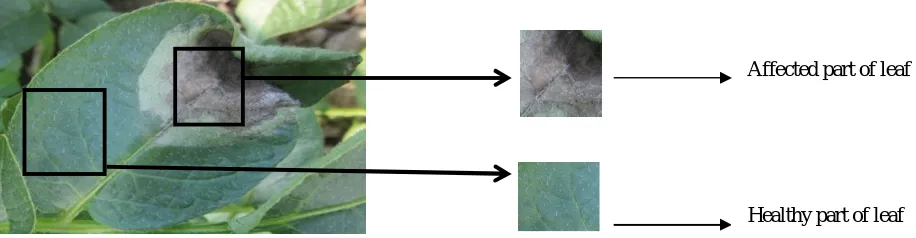
The early symptoms of this disease first appear on leaves within 3 to 5 days. It looks like small, circular or irregularly shaped pale green spots, as dark necrotic lesions [43] (Figure 2A). On the lower side of leaves a white mildew (cottony growth) ring appears around the dead areas. It may first appear on mature lower leaves where low temperature which are most likely to prevail and high humidity or damp conditions. In dry weather, water soaked areas turn necrotic brown. Air can spread spores to healthy plant from nearby infected fields or infected potato plants. On petioles and stems, dark water-soaked lesions appeared (Figure 2B). Infected seed tubers grow into healthy plants but under favourable conditions (10-12 degree C. and RH > 80%) for the disease development.[42] , If we detect this disease in early stage, it will be easy to control its epidemic.

Related works

GLCM was proposed by Haralick(1973)[14] Comprehensive study on extracting spatial information done by Weszka et al.(1976)[17] ,Haralick(1979)[18], Marceau(1989)[19] .They compared the relative capabilities of the gray level co-occurrence matrix method (GLCM), the gray level run length method, the power spectrum method and so many method. Conners and Harlow (1980)[20] also gave a theoretical comparison of based on Weszka et al.(1976)[17] method. Both studies concluded that the GLCM is the most powerful algorithm . Some researcher like Peng Gong[21], P.Mohanaiah[6],Dr. H.B.Kekre[7] use this texture property in classification.

So many researchers have significant contribution to extend moment invariants theory like Dudani et al 1977[26] in Aircraft identification, Wong and Hall, 1978[27] for Scene matching , G.L. Cash and M. Hatamian(1987) [28] in Optical character recognition , W.H. Wong[29] in character recognition, Hais,1981[30] and some high order moment invariants have been explain by Belkasim et al., 1991[31],Wong & Siu (1999)[32]. Muharrem Mercimek[8] use this property in classification.

Principal Components Analysis (PCA)[35] [36] has been successfully applied in a large number of domains such as face recognition [37], coin classification [38], and seismic series analysis [39]..

Jayamala K.Patil[9], S. Ananthi[10], Anand.H.Kulkarni[11], Tushar H Jaware[12], done some similar work on the diseases detection of plant by several method. Shibendu Shankar Ray et al.[13] use the Hyperspectral remote sensing data for crop stress detection. They identify the potato varieties, irrigation level, and early Late Blight diseases detection in potato.

Summary of proposed work

We proposed a system that will detect Late blight disease of potato earlier from analysing its leaves.

II. MATERIALS AND METHODS

Collection of Image data set

Image was collected from potato field at medinipur region of West Bengal India by Dr. Jayanta Tarafdar professor of Directorate of Research, Bidhan Chandra Krishi Viswavidyalaya (BCKB), Kalyani(W.B.) India. He helped us to identifying the Late Blight Disease, affected areas, change in texture, colour and appearance on the image of potato leaf.

Region Of Interest selection

We have to find property of healthy part and affected part of leaf seperatly so our region of interest is as mention below (Fig-4).

Feature Selection and Calculation

GLCM (Gray Level Co-occurrence Matrix method)

Texture Analysis based on statistical properties of intensity histogram like mean standard deviation, energy carry no information regarding the relative position of pixels with respect to each other .But this information is important in texture analysis.

Haralick(1973)[14][15][16] proposed Gray-Tone Spatial-Dependence Matrices which gives information about the

relative position of pixels with respect to each other after that so many spatial feature extraction methods have been

proposed. The Gray Level Co-occurrence Matrix (GLCM)[15] method extracts second order statistical texture features.

Suppose an image of size (MxN) with L possible intensity level. Let G be GLCM a matrix having number of row and

column is equal to number of intensity level(0,1,2,...,L-1) of image And whose element P(i, j,d, ) is the number of Affected part of leaf

Healthy part of leaf

Fig 3 : Flow chart of Early Detection of Late Blight Disease in Potato Input Image

ROI Selection

RGB to GRAY

Feature extraction

Moment invariant GLCM

Classification by PCA Late Blight Disease detected

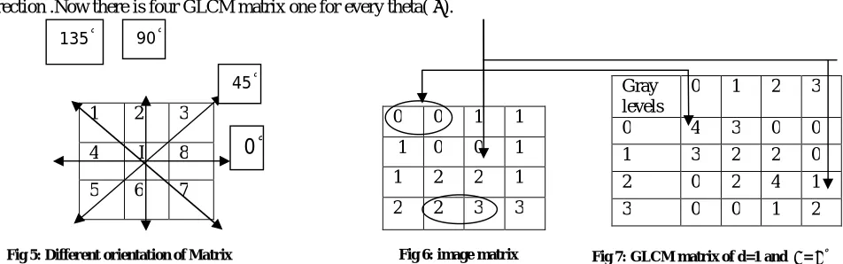
times that the pixel pair separated by d distance in the direction of with intensity i and j occurs on the image .For

d=1(nearest neighbour) there is maximum eight neighbour in a window and = 0°_{, 45}°_{, 90}°_{, 135}°_{cover all eight}

direction .Now there is four GLCM matrix one for every theta( ).

Such that we can find other three GLCM for =45°_{, 90}°_{, 135}°_{. For each matrices, there are so many statistical features}

were obtained like contrast, energy, entropy, homogeneity, correlation and variance. In this paper we consider four important features contrast, energy, homogeneity, correlation [22][23].

CONTRAST: Contrast is a measure of local intensity variation over entire image, away from the diagonal.. For constant image contrast is 0.

ENERGY (uniformity): Energy is the measure of uniformity in range [0, 1]. For constant image it will be 1.

CORRELATION: Correlation is a measure of how correlated a pixel is to its neighbour over entire image. For constant image its value is NAN. Its range is [-1, 1]. Here 1 for perfectly positively correlated and -1 for perfectly negatively correlated image.

Local Homogeneity or Inverse Difference Moment (IDM): Homogeneity is a value that measures the closeness of the distribution of element in the GLCM matrix to the diagonal of GLCM. IDM is influenced by the homogeneity of the image. IDM will get small contributions from inhomogeneous areas. IDM value is low for inhomogeneous images, and a relatively higher value for homogeneous images. Value 1 for a diagonal GLCM matrix and range is [0, 1].

Moment Invariant

The two-dimension moment invariants are the one of the most popular contour-based shape descriptors proposed by M. K. Hu(1962)[24][25]. A set of seven 2-D moment invariants by Hu[24] that are invariant to translation, scale , mirroring (to within a minus sign), and rotation.[33].

The two dimension moment of (p+q)th order of a digital image f(x, y), (where x,y=0,1,2,..M-1) having size (M x N) of is defined as[33][34]

= ( , ) − − − − − − − − −(1)

Where p,q=0,1,2,3....are integers

The central moments of order (p+q) can be expressed as

= ( − ̅) ( − ) ( , ) − − − − − −(2)

Where ̅= =

The central moments are insensitive to translation. For making insensitive to a scale we normalized it. The normalized central moments of (p+q)th order are define as:

= − − − − − − − − − −(3)

1 2 3

4 I 8

5 6 7

Gray levels

0 1 2 3

0 4 3 0 0

1 3 2 2 0

2 0 2 4 1

3 0 0 1 2

0 0 1 1

1 0 0 1

1 2 2 1

2 2 3 3

0

45°

135° ₉₀°

Fig 6: image matrix

Where =( )+ 1 and (p+q)=2,3....

Hu[24-25] define seven 2-D moment invariant based on normalizing central moments of order 3 are define as(eq. 4-10):

∅ = + − − − − − − − − − − −(4)

∅ = ( − ) + 4 − − − − − − − − − − − − − − − −(5)

∅ = ( −3 ) + (3 − ) − − − − − − − − − − − − − − − −(6)

∅ = ( + ) + ( + ) − − − − − − − − − − − − − − −(7)

∅ = ( −3 )( + )[( + ) −3( + ) ] + (3 − )( + )[3( + ) −( + ) ] − − − −(8)

∅ = ( − )[( + ) −( + ) ] + 4 ( + )( + ) − −(9)

∅ = (3 − )( + )[( + ) −3( + ) ] + (3 − )( + )[3( + ) −( + ) ] − − − −(10)

Where ∅ is the moment invariant and ∈(1,2, . .7) .

Principal Components Analysis (PCA)

Principal Components Analysis (PCA)[35] [36] constructs a low-dimensional representation of the data that describes the variance in the data as much as possible. This is done by finding a linear basis of reduced dimensionality for the data, where value of variance of the data is maximal.

III. IMPLEMENTATION AND RESULT

We implement our proposed method through following steps:

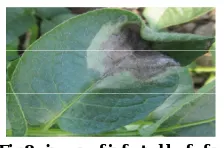
Step 1: Take the images of infected potato leaves form the potato field.

Step 2: ROI select from the taken image such that we can classify visually the healthy and affected region of leaf. Now we take 50 sub image of size (16x16) from healthy and affected parts separately. Size of the sub image may be larger like 27x27 or 64x64 but time complexity will be more because our algorithm of proposed work also depends upon the size of image.

Step 3: Convert the RGB image to Gray scale image because our all feature are based on 2-D calculation.

Step 4: Feature calculation:

We find the texture feature of sub images through these methods: 1. GLCM (Gray Level Co-occurrence Matrix method) 2. Moment Invariant In first method, we find the GLCM matrix of sub image (16x16) where d=1 and = 0°

,45°_{, 90}°_{, 135}°

.For each four important features contrast, energy, homogeneity, correlation are calculated. Such that for four

Fig 8: image of infected leaf of potato

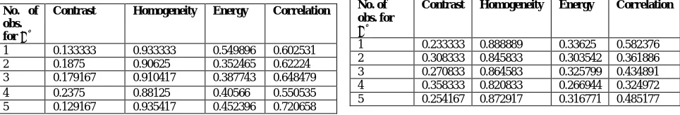
Table 1: Contrast, Homogeneity, Energy, Correlation by GLCM of ° _{orientation of defected part}

No. of obs. for

°

Contrast Homogeneity Energy Correlation

1 0.233333 0.888889 0.33625 0.582376

2 0.308333 0.845833 0.303542 0.361886

3 0.270833 0.864583 0.325799 0.434891

4 0.358333 0.820833 0.266944 0.324972

5 0.254167 0.872917 0.316771 0.485177

In second method, Moment invariants are calculated. Through this method we got seven different features from the sub images of healthy and defected parts separately .These 2-D moment invariant based on normalizing central moments.

Table 3: seven 2-D moment invariants of defected part

No. of

observation

MI (order 1)

MI (order 2)

MI (order 3)

MI (order 4)

MI (order 5)

MI (order 6)

MI (order 7)

1 0.258645 1.89E-05 4.79E-07 4.1E-07 1.58E-13 -5.2E-10 4.79E-14

2 0.265284 5.03E-06 2.1E-06 9.48E-07 1.64E-12 -1.7E-09 2.66E-13

3 0.251371 3.13E-05 3.82E-06 1.16E-05 1.2E-11 3.02E-08 -2E-11

4 0.240952 1.81E-06 3.86E-07 6.1E-06 3.41E-12 7.95E-09 1.54E-12

5 0.254585 2.84E-05 9.33E-06 6.04E-06 4.79E-12 -3E-09 -1.1E-11

Step 5: All features mention in steps 4 have been combined to create the vector contains the different feature values. The step 4 has been repeated for 50 times to take 50 samples.

Table 4: feature matrix (50*23) of healthy part of leaf

No. of sample 1st _{feature 2}nd _{feature 3}rd _{feature 4}th _{feature 5}th _{feature ... 22}nd _{feature 23}rd _feature

1 0.233333 0.888889 0.33625 0.582376 0.204444 .. -1E-08 -3.1E-11

2 0.308333 0.845833 0.303542 0.361886 0.253333 ... -3.7E-08 -4.7E-11

3 0.270833 0.864583 0.325799 0.434891 0.257778 ... -1.7E-09 -2E-12

4 0.358333 0.820833 0.266944 0.324972 0.333333 ... 3.58E-08 7.52E-11

5 0.254167 0.872917 0.316771 0.485177 0.28 ... 8.98E-10 5.7E-13

.. .. .. .. .. .. .. .. ..

.. ... ... ... ... ... .. ... ..

46 0.245833 0.877083 0.270903 0.697679 0.244444 .. 1.05E-07 -5.9E-08

47 0.254167 0.872917 0.327778 0.535068 0.315556 .. -4.5E-07 2.33E-09

48 0.120833 0.939583 0.602535 0.587214 0.186667 .. 7.68E-08 -1.7E-10

49 0.145833 0.927083 0.473368 0.69126 0.182222 .. 7.89E-07 1.08E-08

50 0.204167 0.897917 0.48691 0.420538 0.235556 .. -1.1E-08 -3.4E-11

Table 5: feature matrix (50*23) of defective part of leaf

No. of sample 1st feature 2nd feature 3rd feature 4th feature 5th feature ... 22nd feature 23rd feature

1 0.133333 0.933333 0.549896 0.602531 0.168889 .. -1E-08 -3.1E-11

2 0.1875 0.90625 0.352465 0.62224 0.208889 ... -3.7E-08 -4.7E-11

3 0.179167 0.910417 0.387743 0.648479 0.204444 ... -1.7E-09 -2E-12

4 0.2375 0.88125 0.40566 0.550535 0.235556 ... 3.58E-08 7.52E-11

5 0.129167 0.935417 0.452396 0.720658 0.137778 ... 8.98E-10 5.7E-13

.. .. .. .. .. .. .. .. ..

.. ... ... ... ... ... .. ... ..

46 0.166667 0.916667 0.453125 0.60094 0.195556 .. 4.39E-07 2.42E-08

47 0.129167 0.935417 0.672326 0.405837 0.16 .. 8.12E-08 9.78E-11

48 0.0875 0.95625 0.770868 0.414115 0.088889 .. 1.2E-06 -7E-08

49 0.175 0.9125 0.363576 0.644914 0.204444 .. -1.5E-06 1.53E-08

50 0.1125 0.94375 0.421215 0.766043 0.164444 .. 4.22E-05 3.35E-06

No. of obs. for °

Contrast Homogeneity Energy Correlation

1 0.133333 0.933333 0.549896 0.602531

2 0.1875 0.90625 0.352465 0.62224

3 0.179167 0.910417 0.387743 0.648479

4 0.2375 0.88125 0.40566 0.550535

5 0.129167 0.935417 0.452396 0.720658

Step 6: Principal Component Analysis has been applied on data set obtained from step-5 for feature dimension reduction .we make 50x1 size data by PCA. After that we get the minimum and maximum value. PCA can be summarized in the following steps.

Step 6.1: Feature matrix (50x23) where each column defines a feature vector and each row define a sample have been taken.

Step 6.2: Covariance matrix have been computed. This matrix provides information about the linear independence between the features.

Step 6.3: Eigen values and Eigenvectors have been calculated.

Step 6.4: The contributions of each feature in the total variance have been calculated. The Eigen values of the features whose contribution are greater than or equal to 2.5 have been taken and other are set be zero in eigen value matrix.

Step 6.5: A new matrix P(23*23) has been formed by multiplying eigen value with dot square of its corresponding eigen vectors.

Step 6.6: The individual contributions of each feature have been added to transform the matrix available in Step 9.5 to get a column matrix G(23*1)

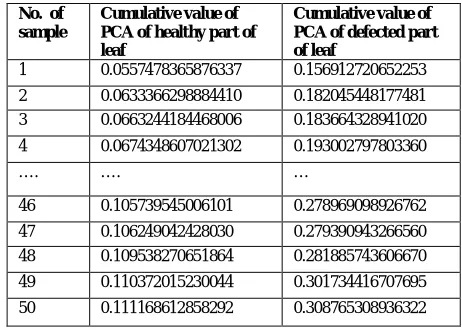
Step 6.7: The transform features have been computed by using = . Where is new feature matrix. The new features are linearly independent. In our calculation of size (50*1) has been formed. Step 6.8: The cumulative value of PCA has been calculated by sorting the value of .(Table 6)

In this example range of healthy part of leaf is 0.05575 to 0.11117 and defected part of the leaf is 0.15691 to 0.30876.Although range will be vary slightly but healthy part and defected part will always classify distinctly.

IV. CONCLUSION

In this project work a system has been designed for early detection and classifications of Late blight (Leaf Blast) disease on potato Leaf. In this schema features of affected leaf images have been extracted. Main feature of images are colour, shape, texture. Total 23 feature of texture like contrast, homogeneity, energy, correlation of GLCM in four orientations and seven set of Moment Invariant have been calculated from Gray scale image of leaves of potato. Dimensions of feature matrix have been reduced by PCA. Cumulative value of reduced dimension matrix gives the range of healthy and defective leaf. This is non overlapping range. Though this values we can classify the different

No. of sample

Cumulative value of PCA of healthy part of leaf

Cumulative value of PCA of defected part of leaf

1 0.0557478365876337 0.156912720652253

2 0.0633366298884410 0.182045448177481

3 0.0663244184468006 0.183664328941020

4 0.0674348607021302 0.193002797803360

…. …. …

46 0.105739545006101 0.278969098926762

47 0.106249042428030 0.279390943266560

48 0.109538270651864 0.281885743606670

49 0.110372015230044 0.301734416707695

50 0.111168612858292 0.308765308936322

Table 6: result after PCA calculation on healthy and defected part

0 0.05 0.1 0.15 0.2 0.25 0.3 0.35

1 5 9 13172125293337414549

cu m u la ti ve v al u e s

no. of samples Comparision

defected

healthy part

group. It is observed that the system detect and classify the healthy and affected spots to an accuracy of 92.46 %. The experimental results show that the proposed schema can recognize the leaf blast diseases with little computational effort. Leaf blight disease is severe epidemic in recent past years. Our proposed method helps in disease control and minimizes the production loss.

REFERENCES

1. McLeod-A., S.-Denman, A. Sadie and F.D.N. Denner.2001. “Characterization of South African isolates of Phytophthora infestans.” Plant Disease 85: 287-91.

2. Sedegui, M., R.B. Carroll, A.L. Morehart., A. Arifi and R. Lakhdar. “First report from Morocco of Phytophthora infestanswith metalaxyl resistance.” Plant disease 81: 831 1997

3. Anonymous.Washington Agricultural Statistics. Washington State Department of Agriculture,Olympia. 1995.

4. Singh, B.P. and G.S. Shekhawat. “Potato Late Blight in India. Technical Bulletin No. 27,” Central Potato Research Institute, Shimla,India. p. 85 1999.

5. M. Narayana Bhat et al., “Assessment Of Crop Losses In Potato Due To Late Blight Disease During 2006-2007” Potato J. 37 (1 - 2): 37-43, 2010.

6. P. Mohanaiah, P.Sathyanarayana, L.GuruKumar, “Image Texture Feature Extraction Using GLCM Approach.” International Journal of Scientific and Research Publications, Volume 3, Issue 5, ISSN 2250-3153, May 2013.

7. Dr. H.B.Kekre et al., “Image Retrieval using Texture Features extracted from GLCM, LBG and KPE .”, International Journal of Computer Theory and Engineering, Vol. 2, No. 5, 1793-8201,October, 2010

8. Muharrem Mercimek et al., “Real object recognition using moment invariants.”, Sadhana Vol. 30, Part 6, pp. 765–775, December 2005. 9. Jayamala K. Patil et al., “Advances In Image Processing For Detection Of Plant Diseases.”, Journal of Advanced Bioinformatics Applications

and Research Vol 2, Issue 2, ISSN 0976-2604, pp 135-141,June-2011.

10. S. Ananthi et al., “Detection And Classification Of Plant Leaf Diseases.”, International Journal of Research in Engineering & Applied Sciences Vol. 2, Issue 2 , ISSN: 2249- 3905, February 2012.

11. Anand.H.Kulkarni et al., “Applying image processing technique to detect plant diseases.” , International Journal of Modern Engineering Research Vol.2, Issue.5,pp-3661-3664 ISSN: 2249-6645, Sep-Oct. 2012.

12. Tushar H Jaware et al., “Crop disease detection using image segmentation.”, World Journal of Science and Technology 2(4):190-194, ISSN: 2231 – 2587, 2012.

13. Shibendu Shankar Ray,J.P. Singh, Sushma Panigrahy., “Use of Hyperspectral Remote Sensing Data For Crop Stress Detection: Ground-Based Studies.”, International Archives of the Photogrammetry, Remote Sensing and Spatial InformationKyoto Japan,Vol-38(8),2010.

14. R. M. Haralick and K. Shanmugam, “Combined Spectral And Spatial Processing Of ERTS Imagery Data,” in Proc. 2nd Symp. Significant Results Obtained from Earth Resources Technology Satellite-I, NASA SP-327, NASA Goddard Space Flight Center,Greenbelt,MD,pp.1219-1228,March 5-9,1973.

15. R. M. Haralick and K. Shanmugam, “Textural Features For Image Classification,” IEEE Trans. Syst., Man., Cybern., vol.SMC-3,pp.610-621,6 Nov.1973.

16. R M. Haralick and R. Bosley, “Texture Features For Image Classification,” Third ERTS Symp., NASA SP-351, NASA Goddard Space Flight Center, Greenbelt, MD, pp. 1929-1969,Dec.10-15, 1973.

17. Weszka, Joan S. , Dyer, Charles R., Rosenfeld, Azriel , “A Comparative Study Of Texture Measures For Terrain Classification,” IEEE Trans. Syst. Man Cybernet. SMC-6(4):269-285,April 1976

18. R. M. Haralick “Statistical and Structural Approaches to Texture,” proceedings of the IEEE, vol. 67, no. 5, pp.786 - 804, May 1979.

19. Marceau, D.J. ,“A Review of Image Classification Procedures with Special Emphasis on the Gray-Level Co-occurrence Matrix Method for Texture Analysis, Earth-Observations Laboratory,” Institute for Space and Terrestrial Science, Dept. of Geography, Univ. of Waterloo, Ontario, Canada, 1989.

20. Conners, R. W., and Harlow, C. A., “A Theoretical Comparison Of Texture Algorithms,” IEEE Trans. Pattern Anal. Mach. Intell. PAMI-2(3):204-222,1980.

21. Peng Gong, Danielle J. Marceau, Philip J. Howarth,“A Comparison of Spatial Feature Extraction Algorithms for Land-Use Classification with SPOT HRV Data.”, remote sens. environ. 40:137-151 (1992).

22. Andrea Baraldi, Flavio Parmiggiani,“An Investigation of Textural Characteristics Associated with Gray Level Cooccurrence Matrix Statistical parameters,” IEEE Trans. On Geoscience and Remote Sensing , vol. 33, no. 2, COM-28, March 1995.

23. Jing Zhang, Gui-li Li, Seok-wum He, “Texture-Based Image Retrieval By Edge Detection Matching GLCM ”, in Proc. of 10th Int. Conference on High Performance Computing and Communications, Sept. 2008.

24. M-K. Hu, “Pattern recognition by moment invariants,” PROC. IRE (Correspondence), vol. 49, p. 1428; September, 1961. 25. Hu M., “Visual pattern recognition by moment invariants.” IRE Trans. Inf. Theor.IT-8: 179–187, 1962.

26. Dudani S A, Breeding K J, Mcghee R B, “Aircraft identification by moment invariants.” IEEE Trans. Comput.C-26: 39–46, 1977. 27. Wong, R.Y. and E.L. Hall. “Scene matching with invariant moments.” Computer Graphics and Image Processing 8, 16-24, 1978.

28. Cash,G.L. and M. Hatamian(1987). “Optical character recognition by the method of moment.” Computer Vision,Graphics, and Image Processing 39,292-310

29. Wai-Hong Wong, Wan-Chi Siu and Kin-Man Lam, “Generation of moment invariants and their uses for character recognition,” Pattern Recognition Letters,16(2), Pages 115-123, February 1995.

30. Haris, T.C. “A note on invariant moments in image processing.” IEEE Trans.Syst. Man Cybernet. 11(12) ,Page 831-834,1981.

32. Wong W H, Siu W C 1999, “Improved digital filter structure for fast moment computation,” IEEE Proc. Vision, Image Signal Process.46: 73– 79

33. R. C. Gonzalez, R. E. Woods, 2004. “Digital Image Processing using MATLAB”, Pearson Education, 2004,

34. Chaur-Chin Chen, “ Improved Moment Invariants For Shape Discrimination.” Pattern Recoonition, 26(5), pp. 683-686, 1993.

35. L.J.P. van der Maaten, E.O. Postma, H.J. van den Herik, “Dimensionality Reduction: A Comparative Review,”.Technical Report, Maastricht University,2007

36. H. Hotelling. “Analysis of a complex of statistical variables into principal components.” Journal of Educational Psychology, 24:417–441, 1933. 37. M.A. Turk and A.P. Pentland. “Face recognition using eigenfaces.” In Proceedings of the Computer Vision and Pattern Recognition 1991,

pages 586–591, 1991

38. R. Huber, H. Ramoser, K. Mayer, H. Penz, and M. Rubik. “Classification of coins using an eigenspace approach.” Pattern Recognition Letters, 26(1):61–75, 2005.

39. A.M. Posadas, F. Vidal, F. de Miguel, G. Alguacil, J. Pena, J.M. Ibanez, and J. Morales. “Spatial-temporal analysis of a seismic series using the principal components method.” Journal of Geophysical Research, 98(B2):1923–1932, 1993.

40. Potato in India Fact file(2003) http://14.139.61.86/ebook-cpri/fact_file.pdf 41. Potato Research in India http://14.139.61.86/ebook-cpri/cpri-brow.pdf 42. Potato Diseases http://nhb.gov.in/vegetable/potato/pot002.pdf