Numerical simulation of paint spray process.

(1)

University of Windsor University of Windsor

Scholarship at UWindsor

Electronic Theses and Dissertations Theses, Dissertations, and Major Papers

1-1-2006

Numerical simulation of paint spray process.

Ligong Yang University of Windsor

Follow this and additional works at: https://scholar.uwindsor.ca/etd

Recommended Citation Recommended Citation

Yang, Ligong, "Numerical simulation of paint spray process." (2006). Electronic Theses and Dissertations. 7229.

https://scholar.uwindsor.ca/etd/7229

This online database contains the full-text of PhD dissertations and Masters’ theses of University of Windsor students from 1954 forward. These documents are made available for personal study and research purposes only, in accordance with the Canadian Copyright Act and the Creative Commons license—CC BY-NC-ND (Attribution, Non-Commercial, No Derivative Works). Under this license, works must always be attributed to the copyright holder (original author), cannot be used for any commercial purposes, and may not be altered. Any other use would require the permission of the copyright holder. Students may inquire about withdrawing their dissertation and/or thesis from this database. For additional inquiries, please contact the repository administrator via email

(2)

NUMERICAL SIMULATION OF PAINT SPRAY PROCESS

By Ligong Yang

A Dissertation

Submitted to the Faculty of Graduate Studies and Research through Mechanical, Automotive and Materials Engineering

in Partial Fulfillment of the Requirements for the Degree of Doctor of Philosophy at

the University of Windsor

(3)

**1*1**

Library and Archives Canada

Published Heritage Branch

395 Wellington Street OttawaONK1A0N4 Canada

Bibliotheque et Archives Canada

Direction du

Patrimoine de I'edition

395, rue Wellington Ottawa ON MAOISM Canada

Your file Votre reference ISBN: 978-0-494-57569-7 Our file Notre r6f6rence ISBN: 978-0-494-57569-7

NOTICE: AVIS:

The author has granted a

non-exclusive license allowing Library and Archives Canada to reproduce, publish, archive, preserve, conserve, communicate to the public by

telecommunication or on the Internet, loan, distribute and sell theses

worldwide, for commercial or non-commercial purposes, in microform, paper, electronic and/or any other formats.

L'auteur a accorde une licence non exclusive permettant a la Bibliotheque et Archives Canada de reproduire, publier, archiver, sauvegarder, conserver, transmettre au public par telecommunication ou par I'lntemet, prefer, distribuer et vendre des theses partout dans le monde, a des fins commerciales ou autres, sur support microforme, papier, electronique et/ou autres formats.

The author retains copyright ownership and moral rights in this thesis. Neither the thesis nor substantial extracts from it may be printed or otherwise reproduced without the author's permission.

L'auteur conserve la propriete du droit d'auteur et des droits moraux qui protege cette these. Ni la these ni des extraits substantias de celle-ci ne doivent etre imprimes ou autrement

reproduits sans son autorisation.

In compliance with the Canadian Privacy Act some supporting forms may have been removed from this thesis.

Conformement a la loi canadienne sur la protection de la vie privee, quelques formulaires secondaires ont ete enleves de cette these.

While these forms may be included in the document page count, their removal does not represent any loss of content from the thesis.

Bien que ces formulaires aient inclus dans la pagination, il n'y aura aucun contenu manquant.

1+1

(4)

(5)

ACKNOWLEDGEMENTS

This work would not have been completed were it not for the tireless patience of my wife, Yuxia. Indeed, were it not for her encouragement, I would not have kept the patience to overcome obstacles in this work.

The person, however, who is most responsible for the vision and quality of this work is Dr. R. M. Barron. Great thanks should be given to him for his guidance and unceasing help during this study.

Thanks goes to Mr. M. A. Malik of DaimlerChrysler Canada, for arranging access to the computer facilities at the University of Windsor/DaimlerChrysler Automotive Research and Development Centre, and for his discussions on various aspects of this study.

Thanks are also due to Dr. G. W. Rankin, Dr. N. Zamani, Dr. P. F. Henshaw and Dr. M. F. Lightstone for evaluating this dissertation as committee members and for their enlightening questions.

Special thanks should be extended to Dr. P. Maksimovic and Dr. E. Koutsavdis of FLUENT for their technical support.

Thanks goes to Mr. C. Tighe of DaimlerChrysler Canada for sharing experimental data with me and to Mrs. B. Mulaosmanovic for creating some of the geometry models.

(6)

ABSTRACT

The electrostatic high-speed rotating bell (ESRB) applicator is widely used in the

automotive finishing industry because of its atomization characteristics and high transfer

efficiency. In order to study the paint spray process of an ESRB, a three-step CFD

simulation methodology has been developed in this research work, using the commercial

CFD code FLUENT. First, the paint flow in the atomizer is simulated, using an Euler

approach. Paint droplet size and velocities at the edge of the atomizer are determined

based on the simulation. Then, the Euler-Lagrange approach is applied to investigate the

droplet transfer process. The air is treated as a continuum and the paint droplets are

tracked as dispersed parcels. Models for electrostatic force and drag force on the droplets,

and droplet breakup and collision models are incorporated in this step. Finally, the paint

film thickness on the target plate and the transfer efficiency are calculated based on the

paint mass accretion on the target plate. The effects that various operating parameters,

such as flow rates, bell rotation speed and voltage, have on the flow field and, in

particular, on the film build and transfer efficiency are examined. The results of the

simulations are compared with experimental observations and data from published

literature and from the paint spray lab at the University of Windsor/DaimlerChrysler

(7)

DEDICATION

(8)

LIST OF TABLES

Chapter 4

Table 4.1 Numerical Simulation Conditions for Paint Flow Rate of 150 cc/min 30 Table 4.2 Numerical Simulation Conditions for Bell Rotating Speed of 38000 rpm 30

Table 4.3 Coefficients and R2 Values of Linear Curve Fit 33

Chapter 5

Table 5.1 Anology between a Spring-Mass System and a Distorting Droplet 42 Table 5.2 Characteristics of Electrostatic Field Domain and Flow Domain 52 Table 5.3 Numerical Simulation Conditions of Droplet Transfer Process for Varying

Electric Charge 55 Table 5.4 Numerical Simulation Conditions of Droplet Transfer Process for Varying

Paint Flow Rate 55 Table 5.5 Numerical Simulation Conditions of Droplet Transfer Process for Varying

Shaping Air Flow Rate 55 Table 5.6 Numerical Simulation Conditions of Droplet Transfer Process for Varying Bell

Rotational Speed 55

Chapter 6

Table 6.1 Summary of the Parametric Study on the Paint Film Thickness and Transfer

(12)

LIST OF FIGURES

Chapter 1

Figure 1.1 Schematic of Typical Automotive Coating Process 2

Figure 1.2 Basecoat Spray Booth 2 Figure 1.3 Perspective and Section View of Paint Spray Nozzle 3

Figure 1.4 Spray Regions 5

Chapter 4

Figure 4.1 Schematic Meridian View of the Bell-shape Atomizer 23

Figure 4.2 Mesh for One Quarter of the Atomizer 25 Figure 4.3 3D Illustration of Paint Film Thickness at the Bell Edge 28

Figure 4.4 Flow Chart for Calculating the Paint Film Thickness at the Bell Edge 29 Figure 4.5 Velocity Vectors on a Meridian Plane of the Bell-shape Atomizer 31 Figure 4.6 Velocity Vectors on a Meridian Plane near the Inlet of the Bell-shape

Atomizer 31 Figure 4.7 Film Thickness at the Bell Edge as a Function of Reynolds Number [from

Domnick & Thieme (2004)] 32 Figure 4.8 Droplet Size vs. Bell Rotation Speed (paint flow rate =150 cc/min) 34

Figure 4.9 Droplet Size vs. Paint Flow Rate (bell rotation speed = 38000 rpm) 35 Figure 4.10 Droplet Axial and Radial Velocities vs. Bell Rotation Speed (paint flow rate

= 150 cc/min) 35 Figure 4.11 Droplet Axial and Radial Velocities vs. Paint Flow Rate (bell rotation speed

= 38000 rpm) 36 Figure 4.12 Droplet Tangential Velocities vs. Bell Rotation Speed (paint flow rate =150

cc/min) 36 Figure 4.13 Droplet Tangential Velocities vs. Paint Flow Rate (bell rotation speed =

38000 rpm) 37 Figure 4.14 Spray Angle vs. Bell Rotation Speed (paint flow rate = 150 cc/min) 37

(13)

Chapter 5

Figure 5.1 Charge-to-Mass Ratio vs. Drop Diameter for the Rotary Bell Atomizer at

40 kV Operating Voltage [from Gemci et al. (2002)] 45 Figure 5.2 Charge-to-Mass Ratio vs. Drop Diameter for the Rotary Bell Atomizer at

70 kV Operating Voltage [from Gemci et al. (2002)] 45 Figure 5.3 Computational Domain for Electrostatic Potential Calculation 48

Figure 5.4 Computational Mesh Distribution for Electrostatic Potential Calculation 48

Figure 5.5 Static Pressure Contours from 2D Air Jet Simulation 49 Figure 5.6 Static Pressure Contours from 2D Air Jet Simulation with Extended Domain50

Figure 5.7 Velocity Magnitude Contours from 2D Air Jet Simulation 50 Figure 5.8 Velocity Magnitude Contours from 2D Air Jet Simulation with Extended

Domain 51 Figure 5.9 Mesh Distribution for Air Flow and Droplet Transfer Simulation 52

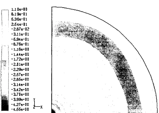
Figure 5.10 Horizontal View of Electric Potential Contours at Z = 0.327 m 57 Figure 5.11 Horizontal View of Electric Potential Contours at Z = 0.2 m 57

Figure 5.12 Meridian View of Electric Potential Contours 58 Figure 5.13 Meridian View of Electric Field Strength Vectors 58 Figure 5.14 Static Pressure Contours on the Target Plate for a Pure Air Spray (shaping air

flow rate = 250 cc/min) 59 Figure 5.15 Meridian View of Air Velocity Vectors (paint flow rate = 1 5 0 cc/min,

shaping air flow rate = 250 cc/min) 60 Figure 5.16 Meridian View of Air Velocity Magnitude Contours (paint flow rate =150

cc/min, shaping air flow rate = 250 cc/min) 61 Figure 5.17 Meridian View of Static Pressure Contours (paint flow rate =150 cc/min,

shaping air flow rate = 250 cc/min) 61 Figure 5.18 Meridian View of Turbulent Kinetic Energy Contours (paint flow rate =150

cc/min, shaping air flow rate = 250 cc/min) 62 Figure 5.19 Meridian View of Turbulent Dissipation Rate Contours (paint flow rate =

150 cc/min, shaping air flow rate = 250 cc/min) 63 Figure 5.20 Static Pressure Contours on the Target Plate (paint flow rate =150 cc/min,

(14)

Figure 5.21 Static Pressure Contours at the Centre of the Target Plate (paint flow rate =

150 cc/min, shaping air flow rate = 250 cc/min) 64 Figure 5.22 Turbulent Kinetic Energy Contours on the Target Plate (paint flow rate = 150

cc/min, shaping air flow rate = 250 cc/min) 65 Figure 5.23 Turbulent Kinetic Energy Contours at the Centre of the Target Plate (paint

flow rate = 150 cc/min, shaping air flow rate = 250 cc/min) 66 Figure 5.24 Turbulent Dissipation Rate Contours on the Target Plate (paint flow rate =

150 cc/min, shaping air flow rate = 250 cc/min) 66 Figure 5.25 Turbulent Dissipation Rate Contours at the Centre of the Target Plate (paint

flow rate = 150 cc/min, shaping air flow rate = 250 cc/min) 61 Figure 5.26 Droplet Trace Coloured by Droplet Residence Time (paint flow rate = 150

cc/min, shaping air flow rate = 250 cc/min) 68 Figure 5.27 Meridian View of Air Velocity Magnitude Contours at 50 kV 69

Figure 5.28 Meridian View of Air Velocity Magnitude Contours at 90 kV 69

Figure 5.29 Static Pressure Contours on the Target Plate at 50 kV 70 Figure 5.30 Static Pressure Contours on the Target Plate at 90 kV 70 Figure 5.31 Droplet Trace Coloured by Droplet Residence Time at 50 kV 71

Figure 5.32 Droplet Trace Coloured by Droplet Residence Time at 90 kV 71 Figure 5.33 Meridian View of Static Pressure Contours using One-tenth of Film

Thickness at the Bell Edge as Initial Droplet Diameter 73 Figure 5.34 Static Pressure Contours on the Target Plate using One-tenth of Film

Thickness at the Bell Edge as Initial Droplet Diameter... 73 Figure 5.35 Turbulent Kinetic Energy Contours on the Target Plate using One-tenth of

Film Thickness at the Bell Edge as Initial Droplet Diameter 74 Figure 5.36 Turbulent Dissipation Rate Contours on the Target Plate using One-tenth of

Film Thickness at the Bell Edge as Initial Droplet Diameter 74 Figure 5.37 Droplet Trace Coloured by Droplet Residence Time using One-tenth of Film

Thickness at the Bell Edge as Initial Droplet Diameter 75 Figure 5.38 Meridian View of Velocity Vectors (bell rotational speed = 42000 rpm) .... 76

(15)

Figure 5.40 Static Pressure Contours at the Centre of the Target Plate (bell rotational

speed = 42000 rpm) 77 Figure 5.41 Turbulent Kinetic Energy Contours at the Centre of the Target Plate (bell

rotational speed = 42000 rpm) 77 Figure 5.42 Turbulent Dissipation Rate Contours at the Centre of the Target Plate (bell

rotational speed = 42000 rpm) 78 Figure 5.43 Meridian View of Static Pressure Contours (paint flow rate = 200 cc/min,

shaping air flow rate = 250 cc/min) 79 Figure 5.44 Static Pressure Contours at the Centre of the Target Plate (paint flow rate =

200 cc/min, shaping air flow rate = 250 cc/min) 79 Figure 5.45 Turbulent Kinetic Energy Contours at the Centre of the Target Plate (paint

flow rate = 200 cc/min, shaping air flow rate = 250 cc/min) 80 Figure 5.46 Turbulent Dissipation Rate Contours at the Centre of the Target Plate (paint

flow rate = 200 cc/min, shaping air flow rate = 250 cc/min) 80 Figure 5.47 Droplet Trace Coloured by Droplet Residence Time (paint flow rate = 200

cc/min, shaping air flow rate = 250 cc/min) 81 Figure 5.48 Meridian View of Static Pressure Contours (paint flow rate = 175 cc/min,

shaping air flow rate = 150 cc/min) 82 Figure 5.49 Static Pressure Contours on the Target Plate (paint flow rate = 175 cc/min,

shaping air flow rate = 150 cc/min) 82 Figure 5.50 Turbulent Kinetic Energy Contours at the Centre of the Target Plate (paint

flow rate = 175 cc/min, shaping air flow rate = 150 cc/min)... 83 Figure 5.51 Turbulent Dissipation Rate Contours on the Target Plate (paint flow rate =

175 cc/min, shaping air flow rate = 150 cc/min) 83 Figure 5.52 Meridian View of Static Pressure Contours (paint flow rate =175 cc/min,

shaping air flow rate = 250 cc/min) 84 Figure 5.53 Static Pressure Contours on the Target Plate (paint flow rate = 175 cc/min,

shaping air flow rate = 250 cc/min) 84 Figure 5.54 Turbulent Kinetic Energy Contours at the Centre of the Target Plate (paint

(16)

Figure 5.55 Turbulent Dissipation Rate Contours on the Target Plate (paint flow rate =

175 cc/min, shaping air flow rate = 250 cc/min) 85 Figure 5.56 Meridian View of Static Pressure Contours (spray angle = 22.5°) 86

Figure 5.57 Static Pressure Contours on the Target Plate (spray angle = 22.5°) 87 Figure 5.58 Turbulent Kinetic Energy Contours at the Centre of the Target Plate (spray

angle = 22.5°) 87 Figure 5.59 Turbulent Dissipation Rate Contours at the Centre of the Target Plate (spray

angle = 22.5°) 88

Chapter 6

Figure 6.1 Paint Accretion on the Target Plate for 0.25 s at the Baseline Operating

Condition (kg/m2) 90

Figure 6.2 Bands Created for Paint Film Thickness Calculation 91 Figure 6.3 Paint Film Thickness Profile and Transfer Efficiency (paint flow rate =150

cc/min, shaping air flow rate = 250 cc/min) 93 Figure 6.4 Predicted Paint Film Thickness Profiles and Transfer Efficiencies for Varying

Electric Charge 94 Figure 6.5 Predicted Paint Film Thickness Profiles and Transfer Efficiencies for Varying

Initial droplet Diameter 95 Figure 6.6 Predicted Paint Film Thickness Profiles and Transfer Efficiencies for Varying

Rotational Speed 95 Figure 6.7 Paint Film Thickness Profile and Transfer Efficiency (paint flow rate =175

cc/min, shaping air flow rate = 250 cc/min) 96 Figure 6.8 Paint Film Thickness Profile and Transfer Efficiency (paint flow rate = 200

cc/min, shaping air flow rate = 250 cc/min) 97 Figure 6.9 Predicted Paint Film Thickness Profiles and Transfer Efficiencies for Varying

Paint Flow Rate (shaping air flow rate = 250 cc/min) 97 Figure 6.10 Paint Film Thickness Profile and Transfer Efficiency (paint flow rate =175

cc/min, shaping air flow rate = 150 cc/min) 98 Figure 6.11 Paint Film Thickness Profile and Transfer Efficiency (paint flow rate =175

(17)

Figure 6.12 Predicted Paint Film Thickness Profiles and Transfer Efficiencies for

Varying Shaping Air Flow Rate (paint flow rate = 175 cc/min) 99 Figure 6.13 Predicted Paint Film Thickness Profiles and Transfer Efficiencies for

(18)

NOMENCLATURE

Q Mass flow rate of paint, kg/s

p Density, kg/m3 pa Density of air, kg/m3 pp Density of paint, kg/m3

R Internal radius of atomizer bell cup at its edge, m

5 Paint film thickness at the edge of atomizer bell cup, m

va Axial velocity of paint, m/s

vr Radial velocity of paint, m/s

vs Tangential velocity of paint, m/s

9 Spray angle or cone angle, degree

d Paint droplet diameter, micron

F Electric force on droplet, N

<f> Electric potential, V

E Electric field strength, V/m

q Electric charge, C

Cv Volumetric solid component ratio

C m Droplet charge-to-mass ratio, C/kg

CD Drag coefficient

Sf Swirl fraction

mj Mass of droplet /, kg

Aj Area of the cell facey, m2

Dj Discrete phase model (DPM) accretion on cell face j , kg/m2 Mk Mass ofpaint accretion on band k, kg

Ak Averaged wet paint film thickness on band k, milliinch (2.54e-5 m)

(19)

gy Gravitational acceleration in y direction, m/s2

g2 Gravitational acceleration in z direction, m/s2

/j Dynamic viscosity, N*s/m2

jua Dynamic viscosity of air, N*s/m2

u Fluid phase velocity, m/s

up Paint droplet velocity, m/s

(20)

CHAPTER 1 INTRODUCTION

Appearance, colour and durability of the painted surface are very important criteria that customers consider when making a decision regarding the purchase of a motor vehicle. Therefore, automotive manufacturers are continuously searching for ways to improve the finish quality of their products. They are also driven by the market, and indirectly by government policy, to increase the transfer efficiency (TE) in the paint spray process and reduce the volatile organic compounds (VOC) emission.

Painting is an expensive process in the automotive industry. A one percent improvement in transfer efficiency (the ratio of the mass of paint deposited on the target object to that injected from the nozzle) of paint spray can save millions of dollars per year because of the savings on paint, energy and resources. Also, in order to protect the environment, automotive producers require low emission of VOC. High transfer efficiency leads to a reduction of VOC emissions and solid waste.

Coating application by means of electrostatic high-speed bell-type rotary atomizers is now widely used in the automotive industry. Compared with the conventional air atomization application, the transfer efficiency is significantly higher. The above factors provide a strong motivation for the study of the paint spray process.

(21)

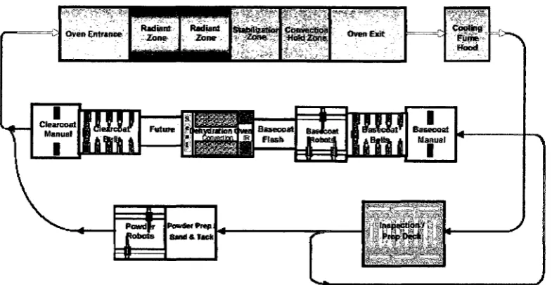
Figure 1.1 Schematic of Typical Automotive Coating Process

Figure 1.2 shows the layout of a basecoat spray booth. The ESRB applicator is installed at the end of each robot. The vehicle is placed in the middle of the booth during spraying.

(22)

Figure 1.3 shows a paint spray gun nozzle with an electrostatic high-speed bell-type rotary atomizer used in a typical paint spray booth. Since water-based paint is used in this study, an indirect electrostatic charge is supplied from six long cylindrical electrodes in an annular locus outside the paint spray gun nozzle. A bell-shape atomizer is installed at the tip of the nozzle. The rotation of the bell cup is driven by compressed air. For the applicator considered in this work, this (turbine) air and the bearing air exhaust along the outer wall of the bell cup, between the bell wall and the shaping air inlet. This exhaust air, along with the shaping air, forms an air curtain that confines the paint spray and increases deposition efficiency.

There is an annular jet ring near the outer rim of the bell cup. During normal operation, jets of paint emerge from the bell cup and the paint undergoes an atomization process, breaking up into droplets. Once airborne, the paint droplets mix with the surrounding air, and droplets collide, break up and coalesce. The flight of the droplets is confined by the air curtain that emerges from the rim of the bell cup. The electrostatic force generated by the positively charged electrodes and the grounded target plate also draws the paint droplets to the plate. Finally, the paint droplets hit the plate and the paint film is generated.

(23)

Researchers have conducted experiments in which paint is sprayed onto a flat plate, and the resulting paint film thickness is measured. In the experimental setup, after the vertical paint spray was fully developed, a rectangular workpiece (target plate) with dimension of 36 inch x 4 inch was passed under the nozzle with a speed of 16 ft/min, i.e., 3.2 inch/s, at a distance of 10 inches from the nozzle. Since the width of the workpiece was 4 inches, it took 1.25 (4-K3.2) seconds for the plate to pass through the paint spray. During this process, paint droplets deposited on the workpiece and formed a thin layer of paint on it. The paint film that had deposited on the plate was then heated until 99 percent of the VOC had been removed. The dry paint film thickness was then measured along the centreline of the rectangular plate.

In order to determine the optimal setting combination to use in the ESRB paint spray process, such as geometric properties of the nozzle and atomizer, voltage of the electrodes, paint and shaping air flow rate, and distance between nozzle and target plate, experimentalists traditionally have to set up costly experiment facilities. These facilities include the particular spray nozzle being tested, high-voltage power source, and expensive light-scattering interferometry instruments, such as a Phase Doppler Anemometer (PDA) and/or a Malvern Particle Sizer. Meanwhile, the testing methods can only obtain data at the exact location where the measurement is taken. For example, PDA can only measure the droplet velocities where the interference area of the laser beams is located. In order to get the droplet properties at any location in the spray, the laser interference area must loop through the whole spray region. Furthermore, measurement difficulties arise in the following aspects: (i) the large amount of droplets in a spray, (ii) the high speed and widely varying velocity of the droplets, (iii) the wide range of droplet sizes encountered in most sprays, and (iv) the changes in droplet size through evaporation, breakup and coalescence. The high cost of building facilities and conducting experiments provides strong motivation for the relatively less expensive Computational Fluid Dynamics (CFD) simulation for the study of the paint spray process.

(24)

droplet/wall interaction region, as illustrated in Figure 1.4. In the disintegration zone, the liquid paint jet from the nozzle is atomized and a very dense spray is generated. Downstream of this atomization region, the spray is assumed to be fully developed, and the droplet/droplet and droplet/air interactions dominate the flow. In the third region, deposition and/or reflection of the droplets occur at the target plate.

The overall objectives of the present study are: (i) to acquire a more detailed and comprehensive understanding of the spray application process, (ii) to develop a methodology for numerical simulation of the paint spray process, (iii) to investigate various factors affecting the paint spray process, and their effect on paint film thickness on the target plate and droplet transfer efficiency, and (iv) to provide suggestions to improve the paint spray process.

Disintegration region

Fully developed spray region

- Droplet/wall interaction region

Figure 1.4 Spray Regions

Three commercial softwares have been used to carry out this study. The CAD model of the atomizer is created with CATIA. The meshes are created with ANSYS ICEM CFD HEXA. The flow simulations are performed and post-processed using FLUENT, which is run on a workstation.

The CFD predictions for the paint film thickness on the target plate and the spray transfer efficiency are compared to the experimental results from the ARDC paint lab.

This dissertation is organized as follows: A survey of the relevant literature is presented in Chapter 2. Sorne general approaches for multiphase simulation are described in Chapter 3. Chapter 4 is devoted to the CFD simulation in the atomizer. Droplet transfer simulation is described in Chapter 5. A method for calculating paint film thickness

Bell £"-:

applicator " :

• • •

-_ — — ^ - U — — - — : — j * = =

(25)

(26)

CHAPTER 2 LITERATURE REVIEW

Sprays are applied in many applications, such as agriculture, fuel injection, pharmaceuticals, powder and liquid paint coatings.

Paint spray is a very complex process. Lefebvre (1989) provided one of the first comprehensive classifications of atomizers and described the general droplet measurement methods and facilities needed for experimental atomization studies. He listed and explained many terminologies used in spray research. These terminologies have now been widely adopted by many researchers. Typically, a spray system consists of three regions: disintegration region, fully developed spray region and droplet/wall interaction region (see Figure 1.4). Most studies reported in the literature are limited to only one of these three parts of the whole spray system.

In order to validate the CFD simulation of the paint spray process, CFD results should be compared with experimental data. Thus, some researchers have set up test facilities to provide the measurements. Others have developed CFD simulation models. In the current study, the rotational speed of the atomizer is very high. Thus, the spray forms a hollow cone close to the edge of the atomizer. Since a pressure-swirl atomizer also generates a hollow cone-shaped spray, some relevant research on pressure-swirl atomizers is reviewed in this chapter. Also, since a properly aligned electrostatic force significantly improves the spray efficiency, review on electrostatic force research cannot be overlooked.

(27)

2.1 Disintegration Region

Different types of atomizers have been employed in various applications. Typical atomizers encountered in industry include the fan atomizer, pressure-swirl atomizer and electrostatic high-speed rotary atomizer. The diversity of the atomizers demonstrates the variety of atomization mechanisms that may occur.

Many researchers have attempted to measure the droplet size in the disintegration region and summarized their results with empirical formulas, or stated their observations on a specific atomizer, e.g., Hinze and Milborn (1950), Bell and Hochberg (1981), Lefebvre (1987), Wang and Lefebvre (1987), St-George and Buchlin (1994), Bailey (1988), Snyder et al. (1989a & 1989b), McCarthy (1991), Corbeels et al. (1992), Bauckage et al. (1994) and Xing et al. (1999). The phase Doppler interferometry technique has been widely used in these studies. The most commonly used equipment for measuring droplet size and velocities are the Laser Doppler Anemometer (LDA), Phase Doppler Anemometer (PDA) and Malvern Particle Sizer (for size only). Unfortunately, no general relationships for the drop size of high-speed rotary atomizers have been proposed by these researchers

Li and Tankin (1988) calculated the droplet size distribution for pressure-swirl atomizers using information theory (or maximum entropy formalism) applied to atomization theory. They obtained a distribution that contains the Weber number as a parameter, and this Weber number is a function of the total number of droplets. The Sauter Mean Diameter (SMD) was also derived as a function of Weber number. Similar methodologies for predicting droplet size have been proposed by Bhatia and Durst (1989) and Van Der Geld and Vermeer (1994). Since the formulas they have proposed contain many geometric parameters of pressure-swirl atomizers, their formulas are not directly applicable to the rotary atomizer studied here.

2.2 Fully Developed Spray Region

(28)

Hicks (1995) and Hicks and Senser (1995) numerically simulated paint transfer in an air spray process by incorporating a number of assumptions based on measurements. The direct effect of turbulent air velocity fluctuations on the trajectories of paint droplets was incorporated via a stochastic separated flow approach. They compared their results with measurements and other published simulation results on the axial air velocity along the centreline of the spray, and the droplet transfer efficiency. They found that their assumptions were valid over broad ranges of atomizing air pressure and liquid flow rate since the shaping air augmented mixing and created a high aspect ratio spray.

Bauckage et al. (1994 & 1995) experimentally investigated the atomization characteristics of a commercial electrostatic high-speed rotary atomizer. The fluid atomized was a water-borne metallic paint typically used in automotive coating processes. Three geometrically different bell types were tested, one with serrations and two without. Axial zones of circulating droplets were observed. They also used a Phase Doppler Particle Analyzer to study the effect of electrostatic force and found that the droplet size was smaller with higher voltage and that the spray cone was wider.

(29)

Only the forces acting on the droplets were considered in their study. They neglected the effect that the droplets have on the air, and did not consider droplet breakup and coalescence. Unfortunately, there was no comparison with experimental data in their study. By employing the Euler-Lagrange approach, similar numerical simulations of the droplet transfer process have been carried out by McCarthy (1995), Bai and Gosman (1995), Dooley et al. (1997), Yarin and Weiss (1995), Mundo et al. (1995c), Ruger et al. (2000), Huang et al. (2000) and Fogliati et al. (2006).

Some researchers have carried out only a numerical investigation on the droplet transfer process. For example, Ellwood and Braslaw (1998) developed a model based on a Lagrangian particle tracking scheme to simulate the formation of spray patterns for charged droplets. Steady state spray patterns were computed using an iterative particle source in cell approach, which represented momentum exchange between the droplet and gas phase as a body force. The flow solver was based on a finite element formulation incorporating the streamlined upwind Petrov Galerkin method for stabilization. They did not provide validation for their simulation based on experimental data. Han et al. (1997) proposed a modified Taylor Analogy Breakup (TAB) model to simulate the breakup of initial blobs and subsequent droplets for the pressure-swirl atomizer and obtained good agreement with experiment. Their model has been adopted by many researchers, and has been incorporated into the commercial CFD code FLUENT for the simulation of droplet breakup.

2.3 Droplet/Wall Interaction Region

(30)

wall, or a droplet on a liquid film, including Pumphrey and Elmore (1990), Oguz and Prosperetti (1990), Trapaga and Szekely (1991), Chandra and Avedisian (1991), Rein (1993), Sommerfeld et al. (1993), Fukai et al. (1993 & 1995), Yarin and Weiss (1995), Cossali et al. (1997), Mao et al. (1997), Mundo et al. (1994, 1995a, 1995b, 1995c & 1998), Tropea and Marengo (1999), Weiss and Yarin (1999), Bussmann et al. (2000).

Numerical simulations on single droplet deformation during impingement, using the Volume of Fluid (VOF) model, have been performed by Ghafouri-Azar et al. (2002) and Garbero et al. (2002).

(31)

2.4 Electrostatic Force in Spray Applications

Electrostatic paint spray application has been a widely used industrial process for many years. The electrostatic charge on spray droplets causes most of the paint to deposit on the workpiece.

The applied potential on the electrodes must be sufficiently high so that an electrostatic field is established in the vicinity of points where air molecules are disrupted by the electrostatic stress into ion-electron pairs. Electrode potentials of a few kilovolts and above are normally used. An electrode at a positive potential attracts negative electrons and repels positive ions away from it, thus behaving as a positive ion source. The positive ions attach to neutral paint molecules to form positive charged paint droplets. Although the electrostatic field is mainly dominated by the electric charge on the electrodes, it is also affected by the charge of the droplets and the movement of the charged droplets (Bailey (1988)).

A thorough and detailed determination of the electrostatic field is very complicated. Following Bailey (1998), Ellwood and Braslaw (1998) and Im (1999), the electrostatic field force F on the charged droplet can be expressed as

F = qE (2.1)

where q is the charge of the droplet and E is the electric field strength, defined as

E = ^- (2.2) ds

where ^ is electric potential and s is distance.

Neglecting the effect of charged droplets on the electrostatic field, the governing

equation for the electric potential is

V V = 0 . (2.3)

The charge on the droplet is determined by many factors, including properties of the liquid, mass of the droplet, surface area of the droplet, strength of the electrostatic field, etc. Although a comprehensive formula for droplet charge is not available,

charge-to-mass ratio {cqm) is a basic parameter that is widely used in charged droplet transfer

(32)

ratio is not uniform to all the droplets in an electrostatic field. Gemci et al. (2002) calculated the individual droplet charge-to-mass ratio based on the drop size and velocity measured with a Phase Doppler Interferometer. He concluded that the droplet size decreased with increasing electric potential.

2.5 Numerical Simulations on Pressure-Swirl Atomizers

Four features are shared by pressure-swirl atomizers and rotary atomizers: (i) the liquid has high swirl near the exit of the atomizers, (ii) a liquid film forms along the atomizer wall near the exit, (iii) a cone of air exists at the centre of the atomizer, and (iv) a hollow cone spray is produced. There are also some important differences between them: (i) the swirling of liquid in pressure-swirl atomizers is caused by the helical channels, whereas the liquid swirling in rotary atomizers results from the rotation of the atomizer wall, (ii) the fluid rotational speed in a rotary atomizer is much higher than in a pressure-swirl atomizer, and (iii) the liquid film thickness at the rotary atomizer edge is

much thinner, and so are the droplet sizes, compared to the pressure-swirl atomizer.

The similarities between the pressure-swirl atomizer and rotary atomizer, and the limited amount of literature on the rotary atomizer, make a review of the research on pressure-swirl atomizers necessary.

Yule and Chinn (1994) proposed a revised inviscid theory to calculate the discharge coefficient and spray angle for the pressure-swirl atomizer. By considering the conservation of axial momentum, this revised theory provided a better basis for the performance analysis and design of pressure-swirl atomizers.

(33)

condition to a 2D two-phase VOF model that solved for the location of the liquid-gas interface. These two-phase flow predictions were linked to experimental images.

Cousin and Nuglisch (2001) presented four models for predicting high pressure-swirl injector performance. A critical review of these models was made by using a huge experimental database where more than 3000 injectors were tested. The authors showed that one of the models predicted the flow rate and cone angle well. These authors also coupled this model with a model that predicted the linear stability of conical sheets. This coupling allowed the determination of a theoretical droplet diameter.

Moriyoshi et al. (2002) used the VOF model to simulate the two-phase flow inside the pressure-swirl injector and the liquid film formation process outside the nozzle. The Discrete Phase Model (DPM) was adopted to simulate a free fuel spray in a constant volume chamber. Multiphase simulation inside the pressure-swirl injector was also carried out by Alajbegovic and Meister (2001).

Chryssakis et al. (2003) developed a comprehensive model for pressure-swirl injectors. The model consisted of pre-spray and main spray modeling. The pre-spray modeling was based on an empirical solid cone approach with varying cone angle. The main spray modeling was based on the Liquid Instability Sheet Atomization approach. Compared with experimental data, some qualitative agreements of spray tip penetration and droplet size were achieved.

2.6 High-speed Rotary Atomizers

Although high-speed rotary atomizers have been investigated by some researchers, most of the published articles are focused on experiments. Some people have developed arguments about the general characteristics of the atomizer, others measured the droplet size. However, no universal formula about droplet size has been proposed.

(34)

(b), or (b) into (c) is caused by an increased quantity of supply, an increased angular speed, a decreased diameter of the cup, an increased density, an increased viscosity, and a decreased surface tension of the liquid.

Bell and Hochberg (1981) studied the atomization, transportation and deposition of coatings of a high-speed electrostatic rotary atomizer. The dynamics of atomization and droplet deposition were examined using high-speed video recording techniques. They measured spray droplet sizes and speeds with laser scattering and Doppler methods. They also calculated the average droplet charge-to-mass ratio.

Corbeels et al. (1992) studied the effect of fluid properties and operational parameters on the atomization of a high-speed rotary bell paint applicator with serrations, using laser diffraction instrumentation and photography. They did not consider the influence of electrostatic force or shaping air. They found that a higher viscosity fluid filmed the bell more evenly and produced long regular ligaments.

Domnick and Thieme (2004) experimentally studied the atomization of the ESRB atomizer. They suggested that the atomization process could be divided into two models, viz., jet disintegration and turbulent disintegration. They also proposed empirical equations to determine the droplet SMD.

2.7 Summary of Previous Studies

Based upon the literature reviewed, the following observations can be made: • Very few simulations of flow in a high-speed rotary atomizer have been

performed.

• Few equations for the prediction of droplet size and velocity for a high-speed rotary atomizer have been proposed.

• Previous simulations of paint spray from a high-speed rotary atomizer are limited to the fully developed spray region.

• In previous droplet transfer simulations, the injected droplet properties have been specified based on experimental droplet size and velocity data.

• The effect of droplets on the air flow has been neglected.

(35)

• According to Gemci et al. (2002), the charge-to-mass ratio varies greatly with the droplet size in an electrostatic field. However, uniform charge-to-mass ratio values have been assumed without justification by previous researchers. • Some researchers described the simulation of single droplet impingement with

a target plate or liquid film. However, no simulation or calculation of paint film build on the target plate has been published.

• There has been little research on whether the impingement and deposition information is applicable to a paint film build calculation. Most of the previous work has focused only on single droplet impingement.

• Very few comparisons of simulated and experimental paint spray transfer efficiency (TE) have been published, although the TE value is one of the most important factors of concern to industry.

• The methodology that Moriyoshi et al. (2002) used is very instructive because it combines the atomization and droplet transfer simulation, although the atomizer they used is a pressure-swirl atomizer, instead of an ESRB atomizer. • Although the atomizer used by Domnick and Thieme (2004) is a rotary

atomizer, it is not the exact same type of atomizer used in the current study. For example, there is no centre hole in their atomizer. Furthermore, the droplet size they proposed was much less than the one used by Im (1999) and Im et al. (2001 & 2004), which was set based on their experimental data.

(36)

CHAPTER 3 M U L T I P H A S E SIMULATION A P P R O A C H E S

The paint spray process under investigation in this study is a multiphase process. The liquid paint is pumped into the nozzle and pushed towards the outer wall of the atomizer by the centrifugal force produced by the high-speed rotation of the bell cup. At the edge of the bell cup, the paint is atomized into droplets. As these droplets move into the spray zone they undergo breakup, coalescence and collision. The trajectories of the droplets are affected by the aerodynamic force exerted by the air and the electrostatic force generated by the charged electrodes and grounded target plate. Furthermore, the charged moving droplets also affect the air flow and the electric field (Bailey, 1998). Finally, the droplets strike the target plate or paint film on the plate, and reflect or deposit onto it. The paint deposited on the plate will further spread out on the plate. Besides paint liquid and air, there are water and volatile organic compounds (VOC) of the paint that evaporate from the paint droplets and paint film on the plate. It is clear that paint spray is a very complex multiphase (paint, vapour and air) process.

Multiphase flow is usually simulated with the Euler approach or the Euler-Lagrange approach. These approaches are described in the next two sections.

3.1 Euler-Euler Approach

In the Euler-Euler approach, the different phases are treated mathematically as interpenetrating continua. Since the volume of one phase cannot be occupied by the other phases, it is convenient to introduce the concept of phase volume fractions. These volume fractions are assumed to be continuous functions of space and time, and their sum is equal to one. Conservation equations for each phase are derived to obtain a set of governing partial differential equations, which have a similar structure for all phases. These equations are closed by providing constitutive relations that are obtained from empirical information or from some theoretical arguments.

(37)

3.1.1 The Eulerian Model

The Eulerian model is the most complex of the multiphase models in FLUENT. The Eulerian multiphase model allows for the modeling of separate, yet interacting phases. The phases can be liquids, gases or solids in nearly any combination, and all phases are treated as continua. For n phases, it solves n sets of momentum and continuity equations, one set for each phase. Coupling is achieved through the pressure and interphase exchange coefficients. The manner in which this coupling is handled depends upon the type of phases involved; granular (fluid-solid) flows are handled differently than non-granular (fluid-fluid) flows. Momentum exchange between the phases is also dependent upon the type of the mixture being modeled. An Eulerian treatment is used for each phase, in contrast to the Eulerian-Lagrangian treatment that is used with the discrete phase model.

With the Eulerian multiphase model, the number of phases is limited only by memory requirements and convergence behaviour. Any number of secondary phases can be modeled, provided that sufficient memory is available. For highly complex multiphase flows, however, the solution may be limited by convergence behaviour.

3.1.2 The Mixture Model

The mixture model is designed for two or more phases (fluid or particulate). As in the Eulerian model, the phases are treated as interpenetrating continua. The mixture model solves one set of momentum equations, referred to as the mixture momentum equations.

The mixture model is a simplified multiphase model that can be used to model multiphase flows where the phases move at different velocities, but assume local equilibrium over short spatial length scales. The coupling between the phases should be strong. It can also be used to model homogeneous multiphase flows with very strong coupling and with the phases moving at the same velocity.

(38)

sedimentation, cyclone separators, particle-laden flows with low loading, and bubbly flows where the gas volume fraction remains low.

The mixture model is a good substitute for the full Eulerian multiphase model in several cases. Implementation of a full multiphase model may not be feasible when there is a wide distribution of a particulate phase or when the interphase laws are unknown or their reliability is questionable. In such cases a simpler model like the mixture model can perform as well as a full multiphase model while solving a smaller number of variables than the full multiphase model.

3.1.3 The VOF Model

The Volume of Fluid (VOF) model uses a surface-tracking technique applied on a fixed Eulerian mesh. It is designed for two or more immiscible fluids where the position of the interface between the fluids is of particular interest. In the VOF model, a single set of momentum equations is shared by the fluids, and the volume fraction of each of the fluids in each computational cell is tracked throughout the domain.

The VOF formulation relies on the assumption that two or more fluids (or phases) are not interpenetrating. For each additional phase added to the model, the volume fraction of the phase in the computational cell is introduced. In each control volume, the volume fractions of all phases sum to unity. The fields for all variables and properties are shared by the phases and represent volume-averaged values, as long as the volume fraction of each of the phases is known at each location. Thus the variables and properties in any given cell are either purely representative of one of the phases, or representative of a mixture of the phases, depending upon the volume fraction values.

Typical VOF applications include the prediction of jet breakup, the motion of large bubbles in a liquid, the motion of liquid after a dam break, and the steady or transient tracking of any liquid-gas interface.

3.2 Euler-Lagrange Approach

(39)

solved by tracking a large number of particles, bubbles, or droplets through the calculated flow field. The fluid and dispersed phases can exchange momentum, mass, and energy.

The Lagrangian discrete phase model (DPM) in FLUENT follows the Euler-Lagrange approach. In addition to solving the transport equations for the continuous phase, FLUENT simulates the discrete second phase in a Lagrangian frame of reference. This second phase consists of spherical particles (which may be taken to represent droplets or bubbles) that disperse throughout the continuous phase. FLUENT computes the trajectories of these discrete phase entities, as well as heat and mass transfer to and from them. Coupling between the phases and its impact on both the discrete phase trajectories and the continuous phase flow can be included. The droplet or particle trajectories can be computed individually at specified intervals during the fluid phase calculation.

A fundamental assumption made in the Euler-Lagrange model is that the dispersed second phase occupies a low volume fraction, even though high mass loading is acceptable.

3.3 Summary

According to the description in sections 3.1.1 - 3.1.3, the Eulerian model should be applied for the simulation of the complete paint spray process. But the reality is that it may not be affordable to use an Euler—Euler approach for the simulation on the whole spray process, due to the high cost associated with such calculations and the available computational resources. On the other hand, the discrete phase model cannot be applied for the whole process because (i) the paint inside the atomizer is continuous and there are no droplets, i.e., no dispersed phase, before atomization, and (ii) the discrete phase model cannot be used to simulate the atomization process.

(40)

droplet properties are then taken to set the boundary and initial conditions for the droplet transfer simulation in the fully developed spray region, using the Euler-Lagrange

(41)

CHAPTER 4 SIMULATION OF FLOW IN THE ATOMIZER

As indicated in previous chapters, a single simulation of the complete paint spray process, from inlet to target plate, is not feasible or practical. In order to simulate the flow in the fully developed spray region (see Figure 1.4), the paint particle size and velocities entering the spray region must be known. Of course, initial droplet sizes and velocities can be obtained through experiment. However, as discussed in Chapter 1, the expense involved in setting up and conducting experiments motivates one to consider a numerical method to acquire these droplet properties. Thus, in this chapter, we develop a numerical procedure to determine the flow in the high-speed rotary bell-shape atomizer, with particular emphasis on predicting the sizes and velocities of paint droplets leaving the outer rim of the bell cup.

(42)

Figure 4.1 Schematic Meridian View of the Bell-shape Atomizer

(43)

the central hole for high rotational speeds. These test simulations show that a dead zone develops at the entrance to the central hole channel, effectively blocking the mixing of the fluid entering through the inlet with that which flows through the channel. Thus, it is reasonable to assume that paint entering the atomizer from the inlet is not significantly affected by the type of fluid (paint or air) sucked in from the central hole of the atomizer at high rotating speeds. The flow of the paint entering from the inlet remains essentially the same regardless of whether a single-phase (pure paint) simulation or a two-phase (paint and air) simulation is performed. This makes it possible to derive the droplet sizes and other flow properties based on a pure paint steady flow simulation in the bell cup.

4.1 The Computational Domain

(44)

Figure 4.2 Mesh for One Quarter of the Atomizer

Numerical Algorithm

The momentum equations of fluid flow are know as the Navier-Stokes equations can be written as

rdu du du du. dp

p{ + W + V + W ) = — + pg^ + / / ( r- + r + T)

dt dx dy dz dx dx dy' dz'

,dv dv dv

s Yu h v —

dt dx dy

3

dp dy

d'u d'u d w,

— 7 + — r + — T

dx dy' dz

d2v d2v d V

p(—+

u

—

+v

—

+w

—) = —r

+

pgv+M(—r+^T+-rT)

- - - - • - chc dy' dz

,dw dw dw dw. dp

p( YU hV + W ) = —+ Pg. + / / (

dt dx dy dz' dz

,d2w d2w d'w

"dx2 dy2 dz2

)

(4.1a)

(4.1b)

(45)

where p is the density of the fluid, p is the pressure, n is the viscosity, u, v, and w

are velocities in x, y, and z directions respectively, and gx, gy and gz are gravitational

acceleration in x, y, and z directions respectively.

FLUENT, which is based on the finite volume method, has been implemented to

solve the 3D Navier-Stokes equations (4.1). The steady state segregated solver, the cell-centre scheme, SIMPLE pressure-velocity coupling and first order upwind discretization

scheme were used. The realizable k - E turbulence model was used rather than the

standard k - 8 turbulence model because of the strong swirl in the bell atomizer. Because the thickness of the paint film (see Figure 4.3) is very small, very fine cells close to the

bell wall are required for the accurate calculation of the film thickness. These small cell sizes along the wall resulted in a small y+ value, which called for the enhanced wall

treatment option in FLUENT. Mass flow rate inlet boundary condition and pressure

outlet boundary condition with "Radial Equilibrium Pressure Distribution" were specified. When the "Radial Equilibrium Pressure Distribution" feature is active, the specified

gauge pressure applies only to the position of minimum radius (relative to the axis of the rotation) at the boundary. The static pressure on the rest of the outlet zone is calculated

from the assumption that radial velocity is negligible, so that the pressure gradient is

given by

^ = ^ i (4.2) dr r

where r is the radial distance from the centre of the bell and ve is the tangential velocity.

4.3 Droplet Properties at the Atomizer Edge

(46)

two-phase (paint and air) simulation is performed. Thus a single-two-phase (paint) simulation has been used to calculate the paint flow characteristics at the edge of the bell cup. The electrostatic field has been neglected since it has no effect on the paint within the atomizer.

Once the simulation has been completed, the blob diameters and velocities at the bell cup edge can be estimated by employing the following steps:

1. Assume an initial film thickness 80.

2. Construct an annular zone at the bell edge plane with outer radius R and inner

radius R-S0, where R is the radius of the bell cup at the edge (see Figure 4.3).

3. From the FLUENT simulation, determine the average axial velocity va of this

annular zone.

4. Calculate the film thickness 8 from the following equation:

S = ^— (4.3) 2nPp{R—±)va

where Q is the paint mass flow rate at the inlet and p is the paint density.

5. If 8 * 80, let S0 = 8 and go to step 2. Otherwise, stop the calculation.

A flow chart of this procedure is described in Figure 4.4.

(47)

(48)

• "

assume ^

0

T

>

\

create annular zone

T

deteiinine v

a

i

compute the fil

thickness s usi

Q

lnp,{R-^X

J

m

ng

<

C

8=

(ei

n o

s ? ^ \

₀_{-^ *•}

yes

k

V*

Figure 4.4 Flow Chart for Calculating the Paint Film Thickness at the Bell Edge

4.4 Simulation Conditions

(49)

different operating conditions, by varying paint flow rate and bell rotating speed. Fixing the paint flow rate at 150 cc/min, the cases given in Table 4.1 were considered.

Bell Rotating Speed (rpm)

25000

30000

34000

38000

44000

50000

55000

60000

Table 4.1 Numerical Simulation Conditions for Paint Flow Rate of 150 cc/min

Specifying the bell rotation speed at 38000 rpm, the simulation cases outlined in Table 4.2 were carried out.

Table 4.2 Numerical Simu

Paint Flow Rate (cc/min) 100

150

200

240

250

300

320

ation Conditions for Bell Rotating Speed of 38000 rpm

4.5 Results and Discussion

(50)

injected at the inlet moves along the outer wall of the bell cup. These velocity vectors are coloured by velocity magnitude (m/s).

:-:3af

l.34cl Z 1.27c02 1.21C02 1.14e'B2 l . ! 7 c ! 2 l . ! l c ! 2 9.39c! l 8.72cl 1 8.15c!l 7.38c! 1 6.7le--n 1 6.04c! 1 5.37c! 1 4.71c! 1 4.13c! 1 3.36c! 1 Z.69c! 1 2.1Zc!l 1.35c! 1 6.79c!! 8.96c! 2 Reversing flow r-'—x Inlet

. — - S i f c S i ' - - , : — • • • : .

'-•.^•fr-'V?'.'

• - • - : - : - . : . * « ? • . • - " ,

> % : \

•^JS5r

7

Outlet

UJ.J t i vv>. i i S.. A v.:

* K

Figure 4.5 Velocity Vectors on a Meridian Plane of the Bell-shape Atomizer

l.34e 1.27e l.Zle 1.14c l . ! 7 c l . l l c 9.39e e.7Ze 6.15ft 7.38e 6 . 7 i c 6.04c 5.37e 4.7!c! 4.03c; 3.36cl 2.69e Z.!2e 1.35c 6.79c 8.96cl !2 12 12 02 02 02 01 01 01 01 01 01 01 01 01 1 01 01 01 Inlet Reversing flow •t-*—x -12

Figure 4.6 Velocity Vectors on a Meridian Plane near the Inlet of the Bell-shape Atomizer

(51)

well with data published by Domnick and Thieme (2004) (see Figure 4.7), which shows the film thickness varying between 15 micron at Reynolds number 106 to around 5 micron at Reynolds number of 107.

t £ H S » 6 l M83&.BS t,#W*frB

Figure 4.7 Film Thickness at the Bell Edge as a Function of Reynolds Number [from Domnick & Thieme (2004)]

The variations of the calculated droplet size with bell rotational speed and paint flow rate are presented in Figure 4.8 and Figure 4.9. These figures indicate that, over the range of parameters considered, the droplet size increases linearly with the paint flow rate and decreases linearly with the rotational speed of the bell cup. This trend was also observed experimentally by Bauckage et al. (1994 & 1995) and predicted numerically by Im (1999) and Im et al. (2004).

The predicted droplet velocities are plotted in Figure 4.10 - Figure 4.13. The droplet velocity magnitude at the edge of the atomizer is dominated by the tangential component, increasing with the increase of bell rotational speed and decreasing as the flow rate increases.

The droplet size and velocities in Figure 4.8 - Figure 4.13 show a linear relation with the horizontal coordinate variables. Using the least square curve fit method, these linear relations can be summarized in the formula

(52)

Table 4.3 shows the coefficients and R2 values of the linear least square curve fit for variables in Figure 4.8 - Figure 4.13.

Relationship

Droplet size vs. bell rotational speed Droplet size vs. paint flow rate

Droplet axial velocity vs. bell rotational speed

Droplet radial velocity vs. bell rotational speed

Droplet axial velocity vs. paint flow rate

Droplet radial velocity vs. paint flow rate

Droplet tangential velocity vs. bell rotational speed

Droplet tangential velocity vs. paint flow rate

Slope a -0.0001 0.0238 2E-05 1E-05 0.0041 0.0021 0.0034 -0.017 Intercept b 12.39 4.5366 0.5673 0.2969 0.7962 0.416 -0.2239 132.75 R2 0.9924 0.9931 0.9933 0.9915 0.9661 0.9731 1 0.9445 Fig. No. 4.8 4.9 4.10 4.10 4.11 4.11 4.12 4.13

Table 4.3 Coefficients and R2 Values of Linear Curve Fit

It can be seen that all the R2 values are close to 1, which indicates there are strong linear relations for these data.

The spray angle 6 is defined as

^ = tan"1(^) (4.5)

where va is the axial velocity of the droplet and vr is the radial velocity of the droplet. The variation of the calculated spray angle with bell rotational speed and inlet flow rate are presented in Figure 4.14 and Figure 4.15. The spray angle is determined by both the

(53)

4.6 Conclusions

This chapter presents a numerical procedure to calculate the paint droplet sizes and velocities at the edge of the high-speed rotary atomizer, by performing a single-phase paint flow simulation inside the bell cup.

The simulations indicate that the droplet size and velocities vary linearly with rotational speed and flow rate. There is no such linearity observed for the spray angle.

The droplet properties obtained through this procedure can be used as inputs for the droplet transfer simulation. The details of droplet transfer simulation will be discussed in Chapter 5. The results indicate that this method is a good alternative to more expensive droplet measurement experiments.

1°

10

~ 8-o

& 6^

E A

n

-( ) 10000

• Droplet size ——Linear (Droplet size)

y =-0.0001 x + 12.39 ^ ^ " " ~ " R2 = 0.9924

20000 30000 40000 50000

i2(rpm)

I

60000 70000

(54)

1 4

12 10

cron

)

O

) 0

0

S

4-- ^ 2 n

0 50

• Droplet size ——Linear (Droplet size)

^ ^ ^ ^

^ ' * " y = 0.0238X + 4.5366

*"" R2 = 0.9931

100 150 200 250 300

Qlp (cc/min)

350

Figure 4.9 Droplet Size vs. Paint Flow Rate (bell rotation speed = 38000 rpm)

2.5 -| 2 ^

1.5-e

w 1

s 0.5 0 -(

• Axial velocity A Radial velocity Linear (Axial velocity) — —Linear (Radial velocity)

y = 2E-05X + 0.5673 m

R2 = 0.9933 ^ a - — " "

•""""""^ ^ - - i

A— • * " * " " * " " y=1E-05x + 0.2969 R2 = 0.9915

) 10000 20000 30000 40000 50000 60000 70000

/2(rpm)

(55)

2.5 2 > 5

H

Axial velocity

•Linear (Axial velocity)

A Radial velocity - —Linear (Radial velocity)

y = 0.0041 x + 0.7962 R2 = 0.9661

y = 0.0021x + 0.416 R2 = 0.9731

50 100 150 200

Q/p (cc/min)

250 300 350

Figure 4.11 Droplet Axial and Radial Velocities vs. Paint Flow Rate (bell rotation speed = 38000 rpm)

S3

250

200

150

100

50

0

• Tangential velocity -^—Linear (Tangential velocity)

y = 0.0034X - 0.2239

10000 20000 30000 40000 50000 60000 70000 /2(rpm)

(56)

132 -, 131.5 131 130.5 "£ 130 1 129.5

w 129

£ 128.5 128 127.5

1 9 7

• Tangential velocity — L i n e a r (Tangential velocity)

•

« N ^ ^ ^ s .

• S* - NN I (^ y = -0.017x+132.75

^S* * > VV N^ R2 = 0.9445

• > ^ ^ ^

^S' VV*

0 50 100 150 200 250 300

Q/p (cc/min)

350

Figure 4.13 Droplet Tangential Velocities vs. Paint Flow Rate (bell rotation speed

38000 rpm)

9 7 R^ _

27.6 ^ 27.55

u

S 27.5 --g 27.45 ^ 27.4

27.35

9 7 "^

-(

1

) 10000 •

20000

• Spray angle

• • • • 30000 40000 /2(rpm) • • +

50000 60000 70000

(57)

1^v

<U 60

<5>

97 R -,

27.55 27.5-27.45

27.4 -27.35 i

27.3 27.25 27.2 27.15 J

(

•

) 50 100

• Spray angle

•

150 200

Q/p (cc/min)

•

• 250

• •

300 350

(58)

CHAPTER 5 DROPLET T R A N S F E R SIMULATION

In the fully developed spray region, the paint droplets can be viewed as dispersed throughout a continuum of air. In order to simulate the paint droplet transfer process, the discrete phase model of FLUENT, following the Euler-Lagrange approach, was adopted. This approach treats the air and droplets as a continuous phase and a dispersed phase respectively, without solving the Navier-Stokes equations for both phases (see details in Chapter 3), which effectively saves computer resources without sacrificing the accuracy of the droplet transfer process simulation. The Euler-Lagrange approach has been adopted by Bai and Gosman (1995), Dooley et al. (1997), Yarin and Weiss (1995), Mundo et al. (1995c), Huang et al. (2000) and Im (1999) and Im et al. (2001 & 2004) for their investigations of the droplet transfer.

In this chapter, descriptions of FLUENT's discrete phase model, spray models, electrostatic force incorporation, turbulent dispersion modeling, computational domain, numerical algorithm and simulation conditions are presented. Then, discussion and comparison of the air flow field and paint trace under various operating conditions are presented.

For figures shown in this thesis, the units corresponding to the numbers on the colour scale are as follows:

• for pressure, Pa

• for velocity magnitude, m/s • for electric potential, V

• for electric field strength, V/m • for droplet residence time, s • for turbulence kinetic energy, m2/s2 • for turbulence dissipation rate, m2/s3

5.1 FLUENT'S Discrete Phase Model

Numerical simulation of paint spray process.

Scholarship at UWindsor

Scholarship at UWindsor

Numerical simulation of paint spray process.

Numerical simulation of paint spray process.

1*1

ACKNOWLEDGEMENTS

ABSTRACT

DEDICATION

TABLE OF CONTENTS

LIST OF TABLES

Chapter 4

Chapter 5

Chapter 6

LIST OF FIGURES

Chapter 1

Chapter 4

Chapter 5

Chapter 6

NOMENCLATURE

CHAPTER 1 INTRODUCTION

Bell *£"-:*

CHAPTER 2 LITERATURE REVIEW

2.2 Fully Developed Spray Region

CHAPTER 4 SIMULATION OF FLOW IN THE ATOMIZER

Numerical Algorithm

3

p(—+

—

—

—) = —r

pgv+M(—r+^T+-rT)

assume ^

create annular zone

deteiinine v

i

compute the fil

thickness s usi

Q

lnp,{R-^X

m

ng

<

C

8=

(ei

n o

s ? ^ \

yes

V*

7

* K

4.6 Conclusions

1.5-e

**1*1**

Bell £"-: