GENETICS | GENOMIC SELECTION
The Causal Meaning of Genomic Predictors and How
It Affects Construction and Comparison of
Genome-Enabled Selection Models
Bruno D. Valente,*,†,1Gota Morota,†Francisco Peñagaricano,†Daniel Gianola,*,†,‡Kent Weigel,* and Guilherme J. M. Rosa†,‡ *Departments of Dairy Science,†Animal Sciences, and‡Biostatistics and Medical Informatics, University of Wisconsin, Madison, Wisconsin 53706
ABSTRACTThe term“effect”in additive genetic effect suggests a causal meaning. However, inferences of such quantities for selection purposes are typically viewed and conducted as a prediction task. Predictive ability as tested by cross-validation is currently the most acceptable criterion for comparing models and evaluating new methodologies. Nevertheless, it does not directly indicate if predictors reflect causal effects. Such evaluations would require causal inference methods that are not typical in genomic prediction for selection. This suggests that the usual approach to infer genetic effects contradicts the label of the quantity inferred. Here we investigate if genomic predictors for selection should be treated as standard predictors or if they must reflect a causal effect to be useful, requiring causal inference methods. Conducting the analysis as a prediction or as a causal inference task affects, for example, how covariates of the regression model are chosen, which may heavily affect the magnitude of genomic predictors and therefore selection decisions. We demonstrate that selection requires learning causal genetic effects. However, genomic predictors from some models might capture noncausal signal, providing good predictive ability but poorly representing true genetic effects. Simulated examples are used to show that aiming for predictive ability may lead to poor modeling decisions, while causal inference approaches may guide the construction of regression models that better infer the target genetic effect even when they underperform in cross-validation tests. In conclusion, genomic selection models should be constructed to aim primarily for identifiability of causal genetic effects, not for predictive ability.
KEYWORDScausal inference; genomic selection; model comparison; prediction; selection; shared data resource; GenPred
O
BTAINING predictors for additive genetic effects (breeding values) is considered pivotal for selection decisions in animal and plant breeding. Such inference is typically obtained byfitting a regression model with predic-tors constructed on the basis of pedigree information or, as became recently common, individual genome-wide genotype information (Meuwissen et al.2001; de los Campos et al.2013a). However, the typical analysis approach for this task involves a contradiction to which little or no attention has been devoted. The incoherence involves interpreting the given predictors as “genetic effects” and using predictive
ability as the primary criteria to evaluate and compare models used to infer such predictors. The conflict is based on the distinction between (a) predicting phenotypes from geno-types and (b) learning the effect of genogeno-types on phenogeno-types. This is an important issue because although a and b are per-formed using regression models, the best models for a may not be the best for b (and vice versa), especially concerning covariate choices and precorrections (Pearl 2000; Shpitser
et al. 2012). Ignoring this distinction might lead one to use
model evaluation criteria that are suitable for a when the target is b and vice versa. Using unsuitable criteria to evaluate models might lead to poor selection decisions.
The aforementioned contradiction can be further described as follows: On one hand, quantitative geneticists present the concept of breeding value mostly under a causal framework. This presentation usually involves a description of how alleles (genotypes) causally affect the phenotype. Their definitions for it often use causal terms such as “causes of variability,”
“influence,” “transmission of values,”and so forth (e.g., Fisher
Copyright © 2015 by the Genetics Society of America doi: 10.1534/genetics.114.169490
Manuscript received March 12, 2015; accepted for publication April 19, 2015; published Early Online April 23, 2015.
Supporting information is available online athttp://www.genetics.org/lookup/suppl/ doi:10.1534/genetics.114.169490/-/DC1.
1Corresponding author: Department of Animal Sciences, 472 Animal Science Bldg.,
1918; Falconer 1989; Lynch and Walsh 1998). The term“ ef-fect,” by itself, is a causal term. Therefore, the meaning of
“genetic effect”indicates that inferring it belongs to the realm of causal inference, where the specification of the regression model (e.g., the decision of covariates to include or not in it) depends on additional (causal) assumptions (Pearl 2000). On the other hand, the inference of genetic effects is generally seen as a prediction task in animal and plant breeding. Meth-ods to tackle prediction problems typically ignore causal assumptions and are insufficient for learning causal effects. Accordingly, discussion on the challenges and pitfalls of causal inference are virtually absent from the literature on these areas, while the issues and terminology belonging to pure prediction are mainstream. Therefore, the way inferences of genetic effects are typically performed indicates that causality is not important for the usefulness of these inferences. As it stands, it seems that the usual approach to inferring genetic effects contradicts the meaning of the information inferred.
Given this conflict, it is not clear if the prevailing analysis approach (for which predictive ability is the most desirable feature) is appropriate for genetic evaluation and selection purposes or if instead models should be evaluated according to identifiability criteria for causal effects inference (Pearl 2000; Spirteset al.2000). Two competing hypotheses regarding this issue are: (a) the usual approach for model evaluation provides the relevant information for selection decisions and any causal denotations from the label given to genomic predictors should not be taken too strictly or (b) selection decisions involve in-ferring and comparing genetic causal effects, and the usual criteria to evaluate models may lead to poor decisions since genomic predictors may not represent genetic causal effects even if they provide good predictive ability. Notice that under the hypothesis b, better identification of genetic causal effects could make including or ignoring covariates and precorrections justifiable even if it means decreasing the genomic predictive ability as evaluated in cross-validation tests. This is important because wrong decisions for covariate choice could result in dramatic changes in values and rankings of predictors, corre-lations between predictors and true genetic effects, values of estimated genetic parameters, and so forth.
Solving this issue refers to assessing if selection decisions ultimately require predictive ability or knowledge on causal effects. In this article we tackle this matter. More specifically, we review the distinction between prediction and causal inference and demonstrate that the genetic causal effect is the target information for selection. We discuss how this implies that the choice of model covariates is important for this inference and why predictive ability does not directly evaluate the perfor-mance of competing regression models to infer genetic effects. Simulated examples under different scenarios are used to il-lustrate this point.
Predictionvs.Causal Inference
One basic distinction important to understanding the in-coherence in the current genomic selectionmodus operandiis
that between prediction and causal inference. Predicting a variable yfrom observing a variable xis not the same as inferring the effect ofxony. This difference is related to the distinction between association and effect (Pearl 2000, 2003; Spirteset al.2000; Rosa and Valente 2013).
The effect ofxonycan be seen as the description of how
ywould respond to external interventions in the value ofx. This is different from the association between these two variables, which can be seen as a description of how their values are related. Consider that qualitative descriptions of how sets of variables are causally related can be expressed using directed graphs, where nodes represent variables and arrows represent causal connections. Ifxaffectsy(x/y), one expected observational consequence is an association between their values. However, a different causal relation-ship could result in the same pattern of association. As a sim-ple examsim-ple, the following four hypotheses are equally compatible with an observed association between xandy: (a)xaffectsy(i.e.,x/y), (b)yaffectsx(i.e.,x)y), (c) bothxandyare affected by a set of variablesZ(i.e.,x) Z / y), and (d) any combination of the previous three hypotheses. Note, however, that each of these hypothetical causal relationships would imply a different response to interventions on x (Pearl 2000; Spirtes et al. 2000; Rosa and Valente 2013). As different causal hypotheses can be equally supported by a given association (or distribution), then the magnitude of a given association is not sufficient for learning the magnitude of a specific causal effect. Mak-ing extra (causal) assumptions would be necessary for that. So it is seen that learning causality is more challenging than learning associational information. The distinction between both tasks lies in the core of the issue here tackled.
More specifically, consider that the linear regression model
REi¼mþHibþeiisfitted. To claim thatbbestimates how the
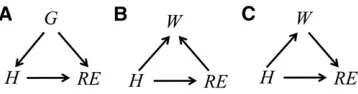
reproductive efficiency trait responds to inoculation of hor-mone, it is necessary to assume that H affects RE and that no other causal path between these two variables contributes to the marginal association explored. However, if another vari-able is assumed to affect bothREandH(e.g., the genotype of a pleiotropic geneG as in Figure 1A), this implies a second pathH)G/REthat would also contribute to the marginal association betweenH andRE. This path, which would also contribute to b^, would represent a source of genetic covari-ance betweenHandREand not an effect ofHonRE. There-fore,fitting the given model does not infer the magnitude of the target causal effect under the assumption expressed in Figure 1A. However, conditioning onGwould block the con-founding path (basic graph theoretical terminology, the asso-ciational consequences of different types of paths in a causal model, and how their contribution to associations change upon conditioning are given in Supporting Information,File S1). Under the same assumption, ^b stemming from fitting
REi¼mþHibþGiaþeicould be claimed as an inferred
ef-fect, as it explores the association betweenREandH condi-tionally on G. However, including covariates is not always beneficial. For example, if it is assumed that bothREandH
affect body weightW(Figure 1B), then there will be again an additional pathH/W)REbetween them. However, this type of path does not contribute to the marginal association. On the contrary, conditioning on a variable that is commonly affected by REandHcreates extra association, which would also contribute tob^if the modelREi¼mþHibþWiaþeiis
fitted. That estimator would not identify the target effect since it explores a conditional association. This model would also be unsuitable if part of the effect ofHonREwas assumed to be actually mediated byW(Figure 1C), as it blocks part of the overall effect one wants to infer. According to the assumptions for the last two cases, the target effect is the only source of the marginal association between H and RE, so that model
REi¼mþHibþeiis the one to be used for causal inference.
While the choice of the model for predictions (and criteria for this choice) could ignore the causal information/assump-tions in Figure 1, it is not possible to choose the model that infers the effect if these assumptions are ignored. Note that statistics are used to infer the magnitude of the effects, but not to learn about the qualitative causal graphs that support their causal interpretation. These relationships cannot be learned from data alone. This indicates that making inferences with causal meaning involves prespecifying causal assumptions (e.g., in terms of directed graphs) and fitting a model that identify (e.g., from an estimated regression coefficient) the
target effect according to those assumptions. Additionally, the choice of the features of the joint distribution to be explored in the inference of causal effects is not related to the strength of the association or to the predictive ability that would result.
Genomic selection analyses typically include (or correct for) covariates but ignore the causal relationships assumed among the variables involved. Additionally, they typically aim
for predictive power. This would be a problem only if it is demonstrated that the relevant information for selection is the effect of genotype on the phenotype and not the ability to predict phenotype from genotype. This issue is tackled in the next section.
The Genetic Effect
In animal and plant breeding, models for genetic evaluation generally assume the signal between genotypes and pheno-types as additive, in which case the term that represents it is called “breeding value” or “additive genetic effect.” In this context, predictors based on genomic information aim at cap-turing this additive signal. The same applies to pedigree-based predictors, but in this article we focus on the genomic selec-tion context. The signal between genotype and phenotype is assumed as additive hereinafter.
The decision on treating the inference of genomic predictors as a prediction problem or as a causal inference is not the same as deciding if there is an effect of genotype on phenotype. In other words, one should not adopt the causal inference approach only because the genotype is believed to affect phenotype. The prediction approach does not assume the absence of such a relationship. The defining point is verifying if breeding programs goals depend on learning causal information or if obtaining predictive ability from genotypes is sufficient for their purpose. In general, learning causal information is required if one must learn how a set of variables is expected to respond to external interventions (Pearl 2000; Spirteset al.2000; Valenteet al.2013). In this section, we investigate if selection requires knowing such information.
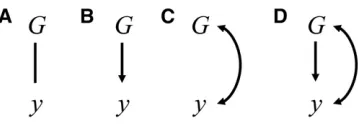
To start, consider the basic structure represented in Figure 2A, in whichGrepresents a whole-genome genotype for some individual, andyis a phenotype. Suppose there is an associa-tion betweenGandybut the causal relationship that generates it is unresolved, so that it is represented by an undirected edge. Selection programs attempt to improve the phenotypeyof individuals of the next generation from modifying their gen-otypes G. This implies that selection relies not only on an association, but on a causal relationship directed from G to
y(such as given in Figure 2B), as the association alone does not justify an expectation of response. Typically, good re-sponse to selection requires choosing which individuals will be allowed to breed in such a way that results in increasing in (next generation’s)Gthe frequency of alleles with desirable effects on y. Considering that phenotypes of individuals re-spond to effects of alleles received from parents, selecting the
best parents depends on identifying individuals carrying alleles with the besteffectson phenotypey(i.e., individuals for which
G have the best effects on y). The essential information for selection is the effect of individualGony. Therefore, for genetic selection applications, genomic predictors should identify a causal effect ofGony. This evaluation is not necessarily the same as identifying individuals with alleles (or genotypes) associated with the best phenotypes, as associations do not necessarily represent effects. Nonetheless, even associations betweenGandythat do not represent the magnitude of the effect of G onycould still be explored for prediction tasks, outside the genetic selection realm.
The distinction between learning effect and association might not be clear when the causal relationships assumed are as in Figure 2B. In that case, the magnitude of the effect ofG
onyis perfectly identified by their marginal association (i.e., identifying genotypes marginally associated with best pheno-types is the same as identifying genopheno-types with best effects on phenotypes). However, this is not the case when there are other sources of association, as discussed ahead. Additionally, spurious associations can be created by bad modeling deci-sions. Interpreting predictors as genetic causal effects, as for any causal inference, involves making causal assumptions about the relationship betweenGandy, and then proposing a model that allows identifying this effect from other possible sources of associations.
To illustrate these concepts, consider a scenario in whichy
is not affected byG(i.e.,yis not heritable), but some aspect of the environment affectsy. Suppose also that relatives tend to be under similar environments. In this case, phenotypes of relatives tend to be more similar to each other due to a com-mon environment effect, and therefore G andy are associ-ated. A graphical representation for this case can be based on the common-cause assumption (Reichenbach 1956): two var-iables can be deemed as commonly affected by a third vari-able if they are mutually dependent but they do not affect each other. As this applies to G and y, the relationship be-tween them can be represented with a double headed arrow (Figure 2C) representing the common cause. Since G and
y are associated, predictions of phenotypes from G can be made (e.g., by using whole-genome regression). However, trying to improve y from modifying G would be useless as there is no causal effect between them. A genomic predictor obtained under this scenario would capture this noncausal signal and, for this reason, it could not be properly inter-preted as genetic effect.
Consider another scenario (Figure 2D) in which the ob-served association betweenGandyis due to a combination of causal and spurious sources. The response ofyto inter-ventions on G would depend only on the causal effect of
Gony, which is not represented by the marginal association between them. Distinguishing the association generated by the causal path from the spurious one(s) would be impor-tant for distinguishing genotypes with best effect onyfrom those simply associated with the best y’s. This task is re-quired to appropriately discriminate the best breeders. But again, when interest refers to the ability to predicty(e.g., an individual’s own performance), any signal could be explored regardless of its sources (e.g., a combination of causal effects and spurious associations).
A simple numerical example consists of two genotypesGA
andGB, each one assigned with expected phenotypic values
2 and 3 units, respectively. This associational information is sufficiently useful for“genomic”prediction: if a genotype
ob-servedfor some individual was equal toGB, then the expected
phenotypic value would be one unit larger than if the
observed genotype was GA. This is equally valid under any
of the structures presented in Figure 2, so no causal assump-tions are required. On the other hand, interpreting the afore-mentioned association as an increase in the expected phenotype by one unit if an individual with genotype GA
had itchangedtoGBwould require assuming that this
asso-ciation reflects a causal effect with no confounding. This requires assuming the causal relationship as in Figure 2B.
In hypothetical simplified scenarios where only genotypes, target phenotypes, and the effects of the former on the latter are included, the inference of genetic effects is not an issue. However, models applied to field data typically incorporate additional covariates. As demonstrated in the section
Predic-tion vs. Causal Inference, including or not, specific covariates
have an important role in the identifiability (i.e., the ability to be estimated from data) of causal effects. This decision should be done to achieve identifiability of the relevant information according to the causal assumptions made. However, this as-pect of the inference task is typically ignored in animal and plant breeding applications, in which the decisions on model construction for breeding values inference are predominantly (and inappropriately) guided by other criterion, such as signif-icance of associations, goodness-of-fit scores, or model predic-tive performance. This is an important issue, because including or ignoring covariates may produce good predictors of pheno-types that are bad predictors of (causal) genetic effects. In the next section we provide simulated examples of how statistical criteria may not provide good guidance for model evaluation when the goal is the inference of breeding values.
Simulated Examples
In this section, we present four simulation scenarios to illustrate how methods for evaluation of predictive ability of models, such as cross-validations, may not indicate the accuracy of inferring genetic effects. For each scenario, we describe why
comparing models with different sets of covariates using predictive ability produced misleading results for selection applications. In the following section, we show how suitable causal assumptions could lead to better choices for each scenario, even if such assumptions are not completely specified (i.e., even if the relationships between some variables are kept as uncertain).
The R (R Development Core Team 2009) script used for such simulation was adapted from Long et al. (2011). The genome consisted of four chromosomes with 1 M each, 15 QTL per chromosome, andfive SNP markers between consec-utive pairs of QTL (320 marker loci). An initial population of 100 diploid individuals (50 males and 50 females) was con-sidered, with no segregation. Polymorphisms were created through 1000 generations of random mating and a probability of 0.0025 of mutation for both markers and QTL. The number of individuals per generation was maintained at 100 until generation 1001, when the population was expanded to 500 individuals per generation. Random mating was simu-lated for 10 additional generations. Data and genotypes for the individuals of the last four generations (2000 individuals) were used for the analyses. Four simulation scenarios were considered, each one with different relationships between the simulated genotypes, phenotypic traits, and other variables. They are outlined below.
Data were analyzed via Bayesian inference with a general model described as
yi¼x9ibþz9imþei; (1)
where yi is a phenotype for a trait recorded in the ith
in-dividual. The model expresses each phenotype as the func-tion in the right-hand side, which includesfixed covariates in x9i, genotypes at different SNP markers recorded on the
ith individual in z9i, and model residuals ei. The column
vectorb containsfixed effects for the covariates in x9i, and mis a vector of marker additive effects, such thatz9imcould be treated as representing the total marked additive genetic effect of theith individual.
For each scenario, there was a variable that could either be included as afixed covariate inx9ior ignored, resulting in two
alternative models differing only inx9ib. These two models are referred to as model C and model IC, standing for covariate and ignoring covariate, respectively. Covariates commonly in-corporated in mixed models include measured environmental factors and phenotypic traits that are distinct from the re-sponse trait. As examples of the latter, a model for studying age at first calving or a behavioral trait in cattle may correct for or account for body weight at a specific age by including it as a covariate, a model for somatic cell score in milk from dairy cows may account for milk yield, a model studyingfirst calving interval may account for age at first calving, and so forth. Popular justifications for including such covariates are reducing the residual variance (leading to more power and precision of inferences), as well as (supposedly) reducing in-ference bias. While we evaluate simple scenarios with only
two alternative models, real applications may involve much larger spaces of models, given the number of potential set of covariates to be considered.
Tofit these models, the R package BLR (de los Campos
et al.2013b) was used. Assuming the residuals of model (1)
as independent and normally distributed, the conditional distribution ofy¼ ½y1 y2 ⋯ yn9is given by
pðyjb;mÞ ¼Y
n
i¼1
pðyijb;mÞeNXbþZm;Is2e;
whereXandZare matrices with rows constituted byx9iand z9i for all individuals, and Iis an identity matrix. The joint
prior distribution assigned to parameters was
pb;m;s2 m;s2e
¼pðbÞpmjs2 m
ps2 m
ps2 e
}N0;Is2m
x22ðdf
m;SmÞx22ðdfe;SeÞ;
where an improper uniform distribution was assigned tob;
Nð0;Is2
mÞis a multivariate normal distribution centered at0
and with diagonal covariance matrixIs2
m, where0is a vector
with zeroes andIis an identity matrix, both with appropri-ate dimensions; andx22ðdf
m;SmÞandx22ðdfe;SeÞare scaled
inverse chi-square distributions specified by degrees of free-dom dfe =dfm=3 and scalesSm=0.001 andSe=1.
The predictive ability was assessed to compare models in the context of genomic prediction studies. We performed 10-fold cross-validation and evaluated two alternative pre-dictive correlations. One of them expresses the associa-tion between observed values yi in the testing set and ^
yi¼x9ib^þz9im^, which is a function of observed values for x9iandz9iin the testing set and the posterior meansb^ andm^
inferred from phenotypes in the training set. This test evaluates the predictive ability from the complete model. The predictive performance was also evaluated by the relation between the phenotype in the testing set cor-rected for fixed effects inferred from the training set (y*
i ¼yi2x9ib^) and the genomic predictorsz9im^. These
pre-dictors are obtained fromz9i observed in the testing set and ^
minferred from the training set. This correlation evaluates the ability of genome-enabled predictors to predict devia-tions from fixed effects. As genetic effects themselves can be viewed as deviations fromfixed effects, the latter test can be judged as more relevant when the goal is predicting breeding values. We have additionally evaluated models according to other relevant aspects depending on the sce-nario. One example is the correlation between genomic pre-dictors z9im^ and the true genetic effect ui, which is the
For the first two scenarios, suppose a trait yD, which is
a continuous trait that indicates the intensity of some disease or pathological process in dairy cattle (e.g., somatic cell count), expressed here with standardized scale (variance equals 1). Suppose that the goal is the selection of individuals with genetic merit for lower levels for the disease trait. In using marker information to predict genomic breeding values, suppose the possibility to correct for (or account for) the effect of milk yield (yM) in the model by including it as a covariate.
Therefore, models IC and C are two alternatives to evaluating individual breeding values for this trait. Typically, alternative models would be compared in terms of their predictive ability, goodness-of-fit, or scores such as AIC (Akaike 1973), BIC (Schwarz 1978), and DIC (Spiegelhalteret al.2002).
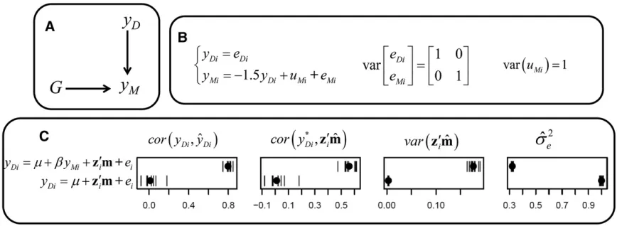
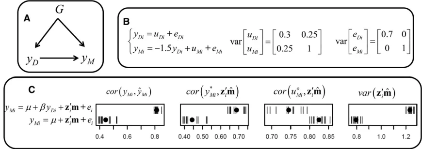
In the first scenario considered, the disease trait was simulated as unaffected by genetics,i.e., it is a nonheritable trait. However, milk yield data were generated as affected by genetics. Additionally, the disease level had an effect on milk yield. The causal graph that expresses this simulation struc-ture is given in Figure 3A, and the sampling model used can be written as a recursive mixed effects structural equation model (Gianola and Sorensen 2004; Wu et al. 2010; Rosa
et al.2011) as specified in Figure 3B. The usual criteria to
evaluate models (ignoring causal relationships) suggest that model C is the best model (Figure 3C), as it predicts disease levels more accurately [corðyDi;^yDiÞ], additionally providing
better predictions of deviations from expected phenotype given fixed effects [corðy*
Di;z9im^Þ]. Furthermore, it resulted
in more variability of the genomic predictors (z9im^) and,
consequently less variability for the residuals. This is com-monly deemed as a good feature, as if the genomic term explained a larger proportion of the true genetic variability ofyD. On the other hand, model IC provides poor predictive
ability from genomic information. However, if one is inter-ested in selection, then model IC is actually the best one because it provides genetic predictors that better reflect the genetic causal effects, or in this case, their absence. Genomic prediction based on model C provides better per-formance on cross-validation tests, but interpreting its pre-dictors as reflecting genetic effects is misleading, suggesting that the disease levels, which is actually nonheritable, would respond to selection. This result comes about because, in this model, the genomic predictor captures the signal be-tween the genome-wide genotype and disease levels condi-tionally on milk yield. Conditioning on a variable affected by both G andyDactivates the path G/yM)yD. This creates
a nonnull signal between genotypes and yD that does not
reflect a causal effect, although it can be explored by geno-mic predictors and successfully used for prediction. On the other hand, the model IC does not create such a spurious association, as its genomic predictors explore the marginal associations between the genotype and yD, which is null,
reflecting the absence of effect.
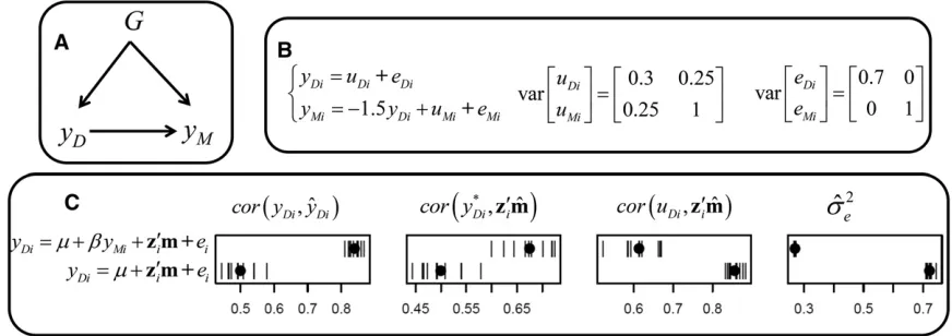
A second scenario considered was similar to the previous one, but assigning also nonnull genetic effects toyD(Figure 4,
A and B). The same alternative models for obtaining
genome-enabled predictions foryDwere compared. In this scenario,
disease levels could potentially respond to selection, but the optimization of this response would depend on the accuracy in inferring the true causal genetic effects. As in the last sce-nario, model C provides the best predictive ability according to corðyDi;^yDiÞ and corðy*Di;z9im^Þ, as depicted in Figure 4C.
However, the correlation between predicted genetic effects and true genetic effects [corðuDi;z9im^Þ] indicates that model
IC better identifies the target quantity. This takes place be-cause for this scenario, there are no other sources of marginal associations betweenGandyDaside fromG/yD. Therefore,
the marginal association reflects the target effect, which is correctly explored by model IC. On the other hand, the ge-nome-enabled predictors from model C explore the associa-tion betweenGandyDconditional onyM. The pathG/yD
contributes to these genetic predictors, but a second source of association betweenGandyDis created due to conditioning
on yM, activating G / yM ) yD. The signal explored by
predictors from model C corresponds to a combination of both active paths. The contribution of this noncausal signal improves predictions of disease levels (as reflected in cross-validation), but harms the ability to infer the genetic effects. Model IC performs worse in the cross-validations tests, but its predictors are not confounded.
In a third scenario (Figure 5, A and B), the sampling model was similar to the last scenario, but here suppose the interest is on selecting for milk yield. Note that the target quantity is the additive genetic effects affecting milk yield, but they are not represented byuMiin Figure 5B. This variable represents
only the genetic effects on yMthat are not mediated by yD.
However, genetics also affect yMthroughG /yD/ yM. In
general, the response to selection on a trait depends on the overall effect of the genotype on that trait, regardless if effects are direct or mediated by other traits (Valente et al. 2013). Therefore, the target of inference here is not uMi, but
uo
Mi¼ 21:5uDiþuMi. Here again, the preferred model
according to the standard cross-validation results (model C) is less efficient in inferring genetic effects. Including yD as
a covariate blocks one of the paths that constitute the target effect, changing the association captured by zim^ in model C (in this case, it reflects the effects of G on yMthat are not
mediated by yD). As a result, just part of the causal effect
sought is captured. On the other hand, model IC does not block this path, and although it is less efficient in predicting disease levels, the genetic effects are better identified by its genomic predictors.
part of the causal genetic effects would result in less genetic variability captured. However, this is not the case if direct genetic effects on traits are positively associated and the causal effect between traits is negative (as applied in this simulation scenario), or vice versa. In this case, blocking one causal path may increase the variability of the predic-tors. However, they should not be blocked when the target is inferring the overall effect, even if it is given by the combi-nation of two“antagonist”causal paths. (SeeFile S1.)
In the fourth and last scenario considered here (Figure 6, A and B), suppose interest is again on genetic evaluation for disease levels. Data are gathered from four farms, and two alternative models include (C) or not (IC) the farm as a cat-egorical covariate in the model. For the simulation, we em-ulated a setting whereyDis affected not only byG, but also
by the farms (Figure 6B) according to the following effects:
F1¼ 23;F2¼ 21;F3¼1;F4¼3. However, consider here
that the farms that are better at controlling for the disease levels tend to have individuals with higher genetic merit for milk yield. Since genetic correlation between disease levels and milk yield is positive, the best farms (lowestFi) will tend
to have the animals that are genetically more prone to high disease levels. The distribution of true genetic effects for disease incidence jointly with the four farm effects is pre-sented in Figure 6B. This relationship between G andyDcan
be represented as a backdoor path G 4 F/ yD, which
additionally contributes to the marginal association between them, and is antagonist to G / yD. Results in Figure 6C
indicate that although model C provides better predictions ofyD, model IC is much better at predictingy*D. Additionally,
fitting model IC suggests greater genetic variability than model C. However, conditioning onFblocks the confound-ing pathG4F/yDthat confounds the inference of genetic
effects. For this reason, in this case model C results in better identification of target genetic effects [corðuDi;z9im^Þ].
Al-though model IC indicates the possibility of a more intense
response to selection than model C does, the negative cor-relation between the genomic predictor and the target effect reveals that adopting this model for selection decisions would possibly result in negative response. This indicates that individuals with negative genetic merit for disease level actually tend to be associated with highyDvalues, as
asso-ciation due to G 4 F / yD not only is antagonist to the
genetic effects but the former outweighs the latter.
Ignoring causal assumptions and considering predictive ability as the major criterion to evaluate models may have important practical consequences for breeding programs. Bad modeling choices for the first simulated scenario (Figure 3) could result in attempting to select for disease level, a non-heritable trait. Selection decisions using inferences provided by the best predictive model for the subsequent two scenarios (Figure 4 and Figure 5) would result in some response to selection for disease level and milk yield, as predictors would still be positively correlated with the true genetic effects. However, as these models provide poorer identification of individuals with the best true genetic effects (i.e., less accu-rate inference of genetic merit), the response to selection would be lower. Finally, the model that is best at predicting deviations from fixed effects attributes much more genetic variability to disease level than it truly has for the fourth simulated scenario. Using predictors from this model would not only result in a disappointing magnitude of response to selection, given the suggested genetic variability, but would actually involve a negative response to selection.
These examples illustrate that, in essence, traditional methods used for model comparison do not evaluate the quality of the inference of the genetic effects. It is not implied that they always point toward the worst model. Of course, in many other instances with different structures and parameter-izations, these comparison methods would eventually point toward a suitable model. However, the simulations were used
as exempla contraria to show that pure genomic predictive
Figure 3 (A) Causal structure, (B) causal model used for simulation, and (C) results fromfitting alternative models. In A,Grepresents the whole-genome genotype, andyDandyMrepresent phenotypes for disease level and milk yield, respectively. In B,yDiandyMiare phenotypes and,eDiandeMiare residuals for the
same traits, anduMiis the genetic effect for milk yield, all of them assigned to theith individual. In C, results are presented for predictive ability of phenotypes
[corðyDi;byDiÞ] and of deviations fromfixed effects [corðy*Di;zi9m^Þ]), for variability of genomic predictors [varðz9im^Þ] and residual variance posterior mean (bs2e). Each
ability is not the main point for breeding programs. The ability to predict as assessed in cross-validations is not sufficient to judge a model as useful for selection.
Using Causal Assumptions for Model Evaluation
This study indicates that models used to infer genetic effects for selection should be deemed as appropriate or not according to the discussion presented in Prediction vs. Causal Inference: one might define qualitative causal assumptions involving the variables studied in the form of causal graphs and then verify if the signal explored by a regression model identifies the target effect according to these assumptions. Many times, however, the correct decision can be reached even if the causal structure is not completely defined, as presented here.
Correct causal structures assumed for thefirst and second scenarios (i.e., assumed as in Figure 3A and Figure 4A) would forbid including milk yield as a covariate in the model. The assumptions indicate that including this covari-ate would crecovari-ate an association from noncausal sources be-tween disease level and the genotypes, by activating the path G /yM)yD. The model IC would be preferred on
this basis. Correct assumptions for the third scenario would indicate that disease levels mediate part of the genetic effect on milk yield, so that including it as a covariate would make the genomic predictor explore only the associations due to the direct genetic effect. As the overall effect is typically the relevant information for selection and the marginal associa-tion between G and yM identifies the magnitude of such
effect (according to the assumption), the model IC should be preferred in this scenario as well. Correct causal assump-tions made for scenario 4 would indicate that two paths contribute to the marginal association between genotype and disease, and therefore models where genomic predic-tors explore it (e.g., model IC) should be avoided. On the other hand, conditioning on farm effect blocks the
con-founding path, suggesting the inclusion of farm as a covari-ate in this case.
Although having a completely specified causal assumption makes decisions more straightforward, many times it is hard to have high confidence on the assumptions of each and every relationship between pairs of variables. Consider again the goal of performing genetic evaluation for disease levels. It is not hard to assume that genotypes may affect traits and not the other way around, but one might not feel as confident in assuming that disease affects milk yield. One might not be willing to completely rule out the hypothesis that milk yield affects disease levels or that there is one (or a set of) hidden variable(s) affecting both of them, resulting in nongenetic associations (Figure 7, A and B). However, for this case, the uncertainty regarding these hypotheses does not change the modeling decision. Under all these hypotheses, including milk yield would harm the identifiability of the target effect from the genomic predictor. It would either activate a noncausal path (Figure 4A and Figure 7B) or block part of the genetic effect (Figure 7A), confounding the inferences. The choice for model IC would be justifiable even under the absence of a com-plete and definite causal assumption, based only on the simple assumption that milk yield is heritable. Note again that this decision is justifiable given the causal assumptions, regardless of the genomic predictive ability obtained from model C.
On the other hand, if competing causal assumptions leaded to different models, one might use different regression models and have alternative genetic evaluations. It would be interesting to compare selection decisions on the basis of the alternative models to verify how much they would differ. Additionally, if there is uncertainty regarding the relationships between some pairs of variables and if different assumptions regarding these relationships result in very different inferences of genetic effects, then good decisions would require efforts on investigating these relationships somehow. This theoretically indicates additional advantages of learning causal relationships
Figure 4 (A) Causal structure, (B) causal model used for simulation, and (C) results fromfitting alternative models. In A,Grepresents the whole-genome genotype, andyDandyMrepresent phenotypes for disease level and milk yield, respectively. In B,yDiandyMiare phenotypes,uDianduMiare genetic effects, and
eDiandeMiare residuals for the same traits, all of them assigned to theith individual. In C, results are presented for predictive ability of phenotypes [corðyDi;^yDiÞ]
and of deviations fromfixed effects [corðy*
Di;z9im^Þ], and of the true genetic effects [corðuDi;z9im^Þ], as well as the residual variance posterior mean (bs2e). Each of
between phenotypic traits for breeding and selection, aside from the ones discussed by Valenteet al.(2013). It should be reminded that under uncertainty on causal assumption that result in alternative models, the goodness-of-fit and the pre-dictive ability is not a direct evaluation of the plausibility of the genetic inferences, as illustrated by the simulated examples.
Here, we have showed how one could use a few rules to verify when a term of a regression model identifies a causal effect. Other cases might involve larger sets of possible covariates, leading to larger spaces of models. However, there are more formal criteria that can be used to make this decision, in the form of lists of rules that should hold for the set of covariates included in the model and the causal assumptions involving the variables (Pearl 2000; Shpitser
et al.2012). This leads to a more systematic way to choose
covariates. The use of such criteria is not focused here since they are richly discussed in the literature. Our goal is only to show why selection requires using criteria of this type and the mistakes that can be made when predictive ability is viewed as the benchmark feature for inference quality.
Discussion
Improving the performance of economically important agri-cultural traits through selection relies on a causal relationship between genotype and phenotypes. Here, we have attempted to demonstrate that obtaining genomic predictors fromfitting a genomic selection model explores an association between these two variables, but these predictors are useful only for selection if the association explored reflects a causal relation-ship. Interpreting these genomic predictors as genetic effects is justifiable only if causal relationships among the studied variables are assumed and if these assumptions indicate that the genetic causal effects are reflected on the association explored by the predictors. We aimed to present the
theoretical basis for this (mostly ignored but intrinsic) feature of genomic selection studies. Differently from methods for prediction, only simulations in which true genetic effects are known could sufficiently shed light on the concepts presented and show how predictive ability tests may not necessarily reflect ability to infer genetic effects.
Much effort on genomic selection research consists of developing new models, methods, and techniques in the context of animal and plant breeding. For example, many parametric and nonparametric models, as well as machine learning methods have been proposed and compared. A comprehensive list of methods and comparisons is given by de los Camposet al.(2013a). Other proposed improvements are using massive genotype data through the so-called next-generation sequencing (Mardis 2008; Shendure and Ji 2008) or alternatively developing low-density and cheaper SNP chips (e.g., Weigelet al.2009), possibly enriched by imputa-tion methods (Weigelet al.2010; Berry and Kearney 2011). As a general rule, the criterion to judge the quality of all methodological novelties is the genomic predictive ability, as assessed by cross-validation. Here we remark that for the purpose of selection programs, the ability to predict is not the point itself, as it may not be relevant if the signal explored does not reflect genetic causal effects. Only after the genetic signal is deemed as causal, increasing the ability to predict such a signal is meaningful.
Selection decisions involve causal questions. Consider for instance an extreme case, where for some reason it is not possible to trust in any causal assumptions that would be necessary for an appropriate choice of covariates. Even so, it is not sensible to react to this limitation by ignoring the causal aspects of the task and blindly explore an arbitrary association for prediction. This choice of approach does not change the fact that selection involves a causal question. In other words, it is not reasonable to answer a question A with
Figure 5 (A) Causal structure, (B) causal model used for simulation, and (C) results fromfitting alternative models. In A,Grepresents the whole-genome genotype, andyDandyMrepresent phenotypes for disease level and milk yield, respectively. In B,yDiandyMiare phenotypes,uDianduMiare genetic
effects, andeDiandeMiare residuals for the same traits, all of them assigned to theith individual. In C, results are presented for predictive ability of
phenotypes [corðyMi;^yMiÞ] and of deviations fromfixed effects [corðyMi* ;z9im^Þ], and of the true genetic effects [corðuMio;z9im^Þ], as well as variability of
genomic predictors [varðz9im^Þ]. Each of these results are given fromfitting models ignoring (Model IC,yMi¼mþz9imþei) or accounting for (Model
the answer for a different question B under the justification that the assumptions to answer B are easier to accept. This conduct still does not answer A. Note that:
a. One needs a causal approach even to express why it is not possible to assume with minimum confidence the causal structure behind a set of variables.
b. If we are using predictors for selectionwe are neces-sarily assuming that information as causal (as we ex-pect response to selection based on that value). c. Declaring that causal assumptions cannot be confirmed
does not imply that causal assumptions can be ignored when predictors of some model (exploring some arbitrary association) are used for selection decisions. It follows from b that such use of genomic predictors implies that they reflect an effect; i.e., the model from which the predictor is obtained identifies the effect. This involves im-plicitly assuming some causal structures that renders the model (predictor) as able to identify the genetic effect. It might be that this implicitly assumed causal structure viola-tes basic biological knowledge (e.g., a structure that assumes that milk yield is not heritable), in which case using the resulting genomic predictors for selection would not be rea-sonable. For a given model, verifying that requires using the concepts presented in the section Prediction vs. Causal
Inference.
From the point of view of interpretation of analysis, note that treating genetic/genomic predictions as a regression problem does not change only the meaning of genomic predictors, but also changes the meaning of other model parameters. For example, following a purely predictive point of view, the estimators for the parameters traditionally named as genetic variance or heritability could not be interpreted as the magnitude of the variability of genetic disturbances. Such interpretation is conditional on treating
predictors as correctly reflecting genetic causal effects. If this is not the case, they could be simply seen as regularization parameters that control the flexibility of a predictive ma-chine. This would be the case of an inferred variance parameter assigned to a model such as GBLUP or a pedigree-based animal model includingyMas covariate under the
sce-nario depicted in Figure 3. This parameter would be expected to be inferred as different from 0, therefore not reflecting the genetic variance of that trait.
Here we do not address the issue of identifying causal loci or distinguishing genomic regions that have more influence on a trait. In other words, the issue is not identifying the effect of a marker or if the regression coefficient of a marker can be interpreted as a function of the effect of a nearby QTL. Although genomic selection models may rely on regressing traits on marker genotypes, we are not conferring any strict causal interpretation to the regression coefficients attributed to each marker. Even in the context of lack of estimability of individual marker regression due to dimensionality (n,,p, as addressed by Gianola 2013), we consider that the signal between the studied trait and the whole-genome genotype can be statisticallyfitted, and it can be interpreted as a ge-nome-wide causal effect. In other words, the difference in the magnitude of this signal attributed to two individuals could be interpreted as the difference of the effect that each whole-genome genotype has on the phenotype. This is the interpre-tation given to genomic predictors when they are used for selection decisions. Such interpretation partially relies on assumptions usually taken in genomic selection studies, as, for example, LD between markers and causal loci. However, this is not sufficient. In thefirst simulation scenario, even if we were using sequence information for a very large sample of data, and a regression model efficient enough to identify individual marker signals with little shrinkage and little
Figure 6 (A) Causal structure, (B) causal model and distribution of effects used for simulation, and (C) results fromfitting alternative models. In A,G represents the whole-genome genotype,yDrepresents phenotypes for disease level, andFrepresents a categorical farm variable. The bidirected edge betweenFandGrepresent a back-door path. In B,yDi,uDi, andeDiare the phenotype, genetic effect, and residuals for disease level, respectively, each
one assigned to theith individual, andFjis the effect of farmj. The graph depicts the dispersion of genetic effects for each category ofF. In C, results are presented for predictive ability of phenotypes [corðyDi;^yDiÞ], of deviations from fixed effects [corðy*Di;z9im^Þ], and of the true genetic effects
[corðuDi;z9im^Þ], as well as variability of genomic predictors [varðz9im^Þ]. Each of these results are given from fitting models ignoring (Model IC,
overfitting, we would still prefer model C based on cross-validation tests.
With the simple simulated examples illustrated here, one might interpret results as a suggestion that heritable traits should never be used as covariates. But this may not be a general rule for covariate choice. Suppose an analysis of individual weaning weight (W) in pigs under a scenario as depicted in Figure 8. In such analysis, litter size (LS) is a pos-sible model covariate and could be seen as a heritable trait of the individual’s dam. However, the genotype of the dam (Gm)
does not affect only the litter size, but also affects the geno-type (G) of the individual through inheritance. From that, including litter size as a covariate blocks, the confounding path betweenGandW, and therefore predictors capture only the direct effect between them. But the overall graph might suggest that genetics also affect weight through LS (although not within a generation, and only through females), but in-cluding LS as a covariates block this effect. For example, to evaluate genetic maternal effects, one might include the ge-notype of the mother as an additional covariate but cannot include LS in the model as it mediates the target effect. Note that the effects of interest could be different depending on the context. Nevertheless, it is not possible to articulate this de-cision only on the basis of associational information (e.g., predictive ability or goodness-of-fit). Another example involves the inclusion of upstream traits, like in the decision involved in the scenario of Figure 5. In a standard scenario, the response to selection would depend on the overall genetic effects. But the inference of direct genetic effects would be useful when predictions are necessary for scenarios under ex-ternal interventions on phenotypic traits (Valenteet al.2013). The information provided by this study did not result from empirical evidences, but from theoretical deductions, sup-ported by simulated examples. Empirical evidence is currently lacking, and it would be a good idea to have it before making dramatic changes in the current approach. Nevertheless, it should also be stressed that the suggestion for changing the approach to evaluating models for selection does not stem from some new theory that we propose, but it was deduced from the theoretic principles that have been used for decades as a basis for selection. In other words, it is the very classic theoretical basis for selection that suggests that identifiability of genetic effects, and not predictive ability, is the target.
Acknowledgments
The authors thank Gary Churchill for providing valuable suggestions. BDV and GJMR acknowledge funding from the Agriculture and Food Research Initiative Competitive Grant no. 2011-67015-30219 from the USDA National Institute of Food and Agriculture.
Literature Cited
Akaike, H., 1973 Information theory and an extension of the max-imum likelihood principle, pp. 267–281 inSecond International Symposium on Information Theory, edited by B. N. Petrov and F. Csaki. Publishing House of the Hungarian Academy of Sciences, Budapest.
Berry, D. P., and J. F. Kearney, 2011 Imputation of genotypes from low- to high-density genotyping platforms and implications for genomic selection. Animal 5: 1162–1169.
de los Campos, G., J. M. Hickey, R. Pong-Wong, H. D. Daetwyler, and M. P. L. Calus, 2013a Whole-genome regression and prediction methods applied to plant and animal breeding. Genetics 193: 327. de los Campos, G., P. Perez, A. I. Vazquez, and J. Crossa, 2013b Genome-enabled prediction using the BLR (Bayesian lin-ear regression) R-package. Methods Mol. Biol. 1019: 299–320. Falconer, D. S., 1989 Introduction to Quantitative Genetics.
Long-man, New York.
Fisher, R. A., 1918 The correlation between relatives on the sup-position of Mendelian inheritance. Trans. R. Soc. 52: 399–433. Gianola, D., 2013 Priors in whole-genome regression: the
Bayes-ian alphabet returns. Genetics 194: 573–596.
Gianola, D., and D. Sorensen, 2004 Quantitative genetic models for describing simultaneous and recursive relationships between phenotypes. Genetics 167: 1407–1424.
Long, N., D. Gianola, G. J. M. Rosa, and K. A. Weigel, 2011 Long-term impacts of genome-enabled selection. J. Appl. Genet. 52: 467–480. Lynch, M., and B. Walsh, 1998 Genetics and Analysis of
Quantita-tive Traits. Sinauer, Sunderland, MA.
Mardis, E. R., 2008 Next-generation DNA sequencing methods.
Ann. Rev. Genomics Hum. Genet.9: 387–402.
Meuwissen, T. H. E., B. J. Hayes, and M. E. Goddard, 2001 Prediction of total genetic value using genome-wide dense marker maps. Genetics 157: 1819–1829.
Pearl, J., 2000 Causality: Models,Reasoning and Inference. Cam-bridge University Press, CamCam-bridge, UK.
Pearl, J., 2003 Statistics and causal inference: a review. Test 12: 281–318.
R Development Core Team, 2009 R: A Language and Environment for Statistical Computing. R Foundation for Statistical Comput-ing, Vienna.
Reichenbach, H., 1956 The Direction of Time. University of Cali-fornia Press, Berkeley, CA.
Rosa, G. J. M., and B. D. Valente, 2013 Breeding and Genetics Symposium: inferring causal effects from observational data in livestock. J. Anim. Sci. 91: 553–564.
Figure 8 Causal structure representing relationships among weaning weight (W), litter size (LS), the genotype of an individual (G), and of its dam (Gm). Arrows represent causal connections.
Rosa, G. J. M., B. D. Valente, G. l. Campos, X. L. Wu, D. Gianola
et al., 2011 2011 Inferring causal phenotype networks using structural equation models. Genet. Sel. Evol. 43: 6.
Schwarz, G., 1978 Estimating dimension of a model. Ann. Stat. 6: 461–464.
Shendure, J., and H. L. Ji, 2008 Next-generation DNA sequencing. Nat. Biotechnol. 26: 1135–1145.
Shpitser, I., T. J. VanderWeele, and J. M. Robins, 2012 On the validity of covariate adjustment for estimating causal effects,
26th Conference on Uncertainty and Artificial Intelligence. AUAI Press, Corvallis, WA.
Spiegelhalter, D. J., N. G. Best, B. R. Carlin, and A. van der Linde, 2002 Bayesian measures of model complexity and fit. J. R. Stat. Soc. Ser. B Stat. Methodol. 64: 583–616.
Spirtes, P., C. Glymour, and R. Scheines, 2000 Causation, Predic-tion and Search. MIT Press, Cambridge, MA.
Valente, B. D., G. J. M. Rosa, D. Gianola, X. L. Wu, and K. Weigel, 2013 Is structural equation modeling advantageous for the genetic improvement of multiple traits? Genetics 194: 561–572. Weigel, K. A., G. de los Campos, O. Gonzalez-Recio, H. Naya, X. L. Wuet al., 2009 Predictive ability of direct genomic values for lifetime net merit of Holstein sires using selected subsets of single nucleotide polymorphism markers. J. Dairy Sci. 92: 5248–5257. Weigel, K. A., G. de los Campos, A. I. Vazquez, G. J. M. Rosa, D.
Gianolaet al., 2010 Accuracy of direct genomic values derived from imputed single nucleotide polymorphism genotypes in Jer-sey cattle. J. Dairy Sci. 93: 5423–5435.
Wu, X. L., B. Heringstad, and D. Gianola, 2010 Bayesian struc-tural equation models for inferring relationships between phenotypes: a review of methodology, identifiability, and appli-cations. J. Anim. Breed. Genet. 127: 3–15.
GENETICS
Supporting Information
http://www.genetics.org/lookup/suppl/doi:10.1534/genetics.114.169490/-/DC1
The Causal Meaning of Genomic Predictors and How
It Affects Construction and Comparison of
Genome-Enabled Selection Models
Bruno D. Valente, Gota Morota, Francisco Peñagaricano, Daniel Gianola, Kent Weigel, and Guilherme J. M. Rosa
File S1
Graph‐theoretic concepts
The structure of how variables are causally related can be represented by a directed graph (Pearl 1995; Pearl 2000)
such as the one depicted in Figure S1. It consists on a set of nodes (representing variables) connected with directed edges
(representing pairwise causal relationships). The connection a→c means that a has a direct causal effect on c. However, causal
effects can be indirect such as the effect of b on e through c (b→c→e). Any sequence of connected nodes where each node
does not appear more than once is called a path (e.g. d←a→c←b, a→d→e). In a path, a collider (Spirtes et al. 2000) is a node
towards which arrows are pointed from both sides (e.g. c in d←a→c←b). Paths can potentially transmit dependence between
nodes on the extremes (active paths). Otherwise, they can be blocked (inactive paths), and therefore transmit no dependence.
Marginally, non‐colliders allow the flow of dependence. For example, in a→d→e there is dependence between a and e. This is
suitable given the causal meaning of this path, since a affects e, and d allows the flow of dependency since it mediates the
causal relationship. Likewise, d and c are expected to be dependent through the path d←a→c. This is expected given that
variable a is a common influence on both d and c, and therefore, a allows the flow of dependence as well. On the other hand, a
collider is sufficient to block a path. For example, in a→c←b, c is commonly affected by a and b, but this does not imply
dependence between this pair (i.e. observing a value for a does not change the expected value for b just on the basis of having
a common consequence in c). Upon conditioning, these properties of colliders and non‐colliders are reversed. This means that
conditioning on non‐colliders blocks the path. For example, in a→d→e, conditionally on knowing the value of d, learning the
value of a does not give any additional information about e. The same goes for d←a→c conditionally on a. On the other hand,
conditioning on colliders turns it into a node that allows the flow of dependence. For example, in a→c←b, once the value of c is
known, then observing the value for a updates the expected value for b. Paths that present marginal flows of dependence
either represent a causal path (e.g. a→d→e) or the so‐called back‐door paths (e.g. d←a→c→e). The latter are marginally active
paths containing both extreme nodes with arrows pointed towards them. Such paths represent a relationship between these
pair of nodes that is not causal, but it is still a source of association. For example, in d←a→c→e, d and e are expected to be
marginally dependent, but interventions in one of them would not lead to modifications in the value of the other.
Although a graph is a good way to encode causal information and assumptions, it only provides a qualitative
representation of causal relationships, and therefore it does not sufficiently specify a causal model. For example, from a→c it is
not possible to deduce the magnitude or sign of the effect and therefore this is not sufficient to determine the resulting joint
A causal graph can be interpreted as a family of causal models from which those qualitative causal relationships can
be deduced. However, by exploring the d‐separation criterion (Pearl 1988; Pearl 2000; d stands for directional), graphs are also
very effective in representing conditional independences among variables that necessarily follow from the causal information
they encode. Two nodes are d‐separated in a graph conditionally on a subset of the remaining nodes if there are no active
paths between them under this circumstance. For example, in Figure 1, a and e are d‐separated conditionally on d and c, as
both paths between these two variables (a→d→e and a→c→e) become inactive in this context. This means that in the joint
probability distribution resulted from any causal model with the given structure, a and e are independent conditionally on d
and c. However, conditioning on only one of either c or d is not sufficient for d‐separation, as one of the paths between a and e
becomes active. Likewise, b and d are marginally d‐separated as both paths between them contain a collider (i.e. d←a→c←b
and d→e←c←b), but they are not d‐separated conditionally on e or on c.
References
Pearl, J., 1988 Probabilistic reasoning in intelligent systems : networks of plausible inference. Morgan Kaufmann Publishers, San
Mateo, Calif.
Pearl, J., 1995 Causal diagrams for empirical research. Biometrika 82: 669‐688.
Pearl, J., 2000 Causality: Models, Reasoning and Inference. Cambridge University Press, Cambridge, UK.
Spirtes, P., C. Glymour and R. Scheines, 2000 Causation, Prediction and Search. MIT Press, Cambridge, MA.
Figure S1 A directed acyclic graph.