The Effect of Strong Purifying Selection on Genetic Diversity

(1)

HIGHLIGHTED ARTICLE

| INVESTIGATION

The Effect of Strong Purifying Selection on

Genetic Diversity

Ivana Cvijovi´c,*,†,1_{Benjamin H. Good,}†,‡,§_{and Michael M. Desai*},†,_**,1 *Department of Organismic and Evolutionary Biology, Harvard University, Cambridge, Massachusetts 02138,†Kavli Institute for Theoretical Physics, University of California, Santa Barbara, California 93106,‡Department of Physics, and§Department of Bioengineering, University of California, Berkeley, California 94720, and **Department of Physics, Harvard University, Cambridge, Massachusetts 02138 ORCID ID: 0000-0002-7757-3347 (B.H.G.)

ABSTRACTPurifying selection reduces genetic diversity, both at sites under direct selection and at linked neutral sites. This process, known as background selection, is thought to play an important role in shaping genomic diversity in natural populations. Yet despite its importance, the effects of background selection are not fully understood. Previous theoretical analyses of this process have taken a backward-time approach based on the structured coalescent. While they provide some insight, these methods are either limited to very small samples or are computationally prohibitive. Here, we present a new forward-time analysis of the trajectories of both neutral and deleterious mutations at a nonrecombining locus. Wefind that strong purifying selection leads to remarkably rich dynamics: neutral mutations can exhibit sweep-like behavior, and deleterious mutations can reach substantial frequencies even when they are guaranteed to eventually go extinct. Our analysis of these dynamics allows us to calculate analytical expressions for the full site frequency spectrum. Wefind that whenever background selection is strong enough to lead to a reduction in genetic diversity, it also results in substantial distortions to the site frequency spectrum, which can mimic the effects of population expansions or positive selection. Because these distortions are most pronounced in the low and high frequency ends of the spectrum, they become particularly important in larger samples, but may have small effects in smaller samples. We also apply our forward-time framework to calculate other quantities, such as the ultimate fates of polymorphisms or the fitnesses of their ancestral backgrounds.

KEYWORDSlinked selection; background selection; distinguishability; allele frequency trajectories; rare variants

P

URIFYING selection against newly arising deleterious mutations is essential to preserving biological function. It is ubiquitous across all natural populations and is respon-sible for genomic sequence conservation across long evolu-tionary timescales. In addition to preserving function at directly selected sites, negative selection also leaves signa-tures in patterns of diversity at linked neutral sites, which have been observed in a wide range of organisms (Begun and Aquadro 1992; Charlesworth 1996; Cutter and Payseur 2003; McVicker et al.2009; Flowers et al.2012; Comeron

2014; Elyashivet al.2016). This process is known as back-ground selection and understanding its effects is essential for characterizing the evolutionary pressures that have shaped a population, as well as for distinguishing its effects from less ubiquitous events such as population expansions or the pos-itive selection of new adaptive traits.

At a qualitative level, the effects of background selection are well known: it reduces linked neutral diversity by reducing the number of individuals that are able to contribute descen-dants in the long run. Since individuals that carry strongly deleterious mutations cannot leave descendants on long timescales, all diversity that persists in the population must have arisen in individuals that were free of deleterious mutations. Since all of these individuals are equivalent in ﬁtness, this suggests that diversity should resemble that expected in a neutral population of a smaller size—speciﬁcally, with a size equal to the number of mutation-free individuals (Charlesworthet al.1993).

Manuscript received April 20, 2018; accepted for publication May 25, 2018; published Early Online May 29, 2018.

Supplemental material available at Figshare: https://doi.org/10.25386/genetics. 6167591.

(2)

However, an extensive body of work has shown that this intuition is not correct and that background selection against strongly deleterious mutations can lead to nonneutral distor-tions in diversity statistics (Charlesworthet al.1993, 1995; Hudson and Kaplan 1994; Tachida 2000; Gordoet al.2002; Williamson and Orive 2002; O’Fallonet al.2010; Nicolaisen and Desai 2012; Walczaket al.2012; Goodet al.2014). The reason for this is simple: even strong selection cannot purge deleterious alleles instantly. Instead, deleterious haplotypes persist in the population on short timescales, allowing neu-tral variants that arise on their backgrounds to reach mod-est frequencies. This is most readily apparent in statistics based on the site frequency spectrum [the number,pðfÞ;of polymorphisms which are at frequencyfin the population], such as the number of singletons or Tajima’s D (Tajima 1989). As we show below, even when deleterious muta-tions have a strong effect on ﬁtness, the site frequency spectrum shows an enormous excess of rare variants com-pared to the expectation for a neutral population of re-duced effective size.

These signatures in genetic diversity are qualitatively sim-ilar to those we expect from population expansions and positive selection (Slatkin and Hudson 1991; Sawyer and Hartl 1992; Rannala 1997; Keinan and Clark 2012). A de-tailed quantitative understanding of background selection is therefore essential if we are to disentangle its signatures from those of other evolutionary processes.

The traditional approach to analyzing the effects of puri-fying selection has been to use backward-time approaches based on the structured coalescent (Hudson and Kaplan 1988, 1994). This offers an approximate framework to model how background selection affects the statistics of genealogical his-tories of a sample, and hence the expected patterns of genetic diversity. The approximations underlying this method are valid when selection is sufﬁciently strong that deleterious mutations rarelyﬁx (Neher and Shraiman 2012), the same regime we will consider in this work. However, while these backward-time structured coalescent methods make it possi-ble to rapidly simulate genealogies, they are essentially nu-merical methods and do not lead to analytical predictions. Furthermore, they give limited intuition as to the conditions under which their approximations are valid. A more technical but crucial limitation is that they rapidly become very com-putationally demanding in larger samples. This is becoming an increasingly important problem as advances in sequencing technology now make it possible to study sample sizes of thousands (or even hundreds of thousands) of individuals. The poor scaling of coalescent methods with sample size is of particular importance in studying background selection: since purifying selection is expected to result in an excess of rare variants, its effects increase in magnitude as sample size increases. This can reveal deviations from neutrality in large samples that are not seen in smaller samples.

Here, we use an alternative, forward-time approach to analyze how purifying selection affects patterns of genetic variation at a nonrecombining genomic segment. Our method

is based on the observation that to predict single-locus statis-tics, such as the site frequency spectrum, it is not necessary to model the entire genealogy. Instead, we model the frequency of the lineage descended from a single mutation as it changes over time due to the combined forces of selection and genetic drift, and as it accumulates additional deleterious mutations. We then use these allele frequency trajectories to predict the site frequency spectrum, from which any other single-site statistic of interest can then be calculated (note, however, that multi-site statistics such as linkage disequilibrium or correlations between allele frequencies at different sites can-not be calculated from the site frequency spectrum).

We show that background selection creates large distor-tions in the frequency spectrum at linked neutral sites when-ever there is signiﬁcantﬁtness variation in the population. These distortions are concentrated in the high- and low-frequency ends of the low-frequency spectrum, and hence are particularly important in large samples. We provide analytical expressions for the frequencies at which these distortions occur and we can therefore predict at what sample sizes they can be seen in data.

Aside from single time-point statistics such as the site frequency spectrum, we also obtain analytical forms for the statistics of allele frequency trajectories. These trajectories have a very nonneutral character which reﬂects the underly-ing linked selection. Our approach offers an intuitive explana-tion for how these nonneutral behaviors arise in the presence of substantial linkedﬁtness variation, which explains the origins of the distortions in the site frequency spectrum.

The statistics of allele frequency trajectories can also be used to calculate any time-dependent, single-site statistic. For example, we analyze how the future trajectory of a mutation can be predicted from the frequency at which we initially observe it, and we discuss the extent to which the observed frequency of a polymorphism can inform us about theﬁtness of the background on which it arose.

We emphasize that we focus throughout on modeling a perfectly linked genomic region. In the presence of recombi-nation, our results offer insights about the effects of linked selection on diversity within regions that are effectively fully linked on the relevant timescales. In theDiscussion, we discuss how our results can be used to provide a lower bound on the length of these segments, and therefore on the amount of linked selection relevant in sexually reproducing popula-tions, and we comment on possible future extensions of our analysis to include recombination explicitly.

(3)

We then present the analysis of our model. We begin by reviewing how dynamical aspects of allele frequency trajec-tories can be related to site frequency spectra, using the trajectories of isolated loci as an example. Readers already familiar with this intuition may choose to skip ahead, but those less interested in the technical details may ﬁnd that this section provides useful intuition for the calculations in a simpler context. We then explain how this approach must be modiﬁed to account for linkage between multiple selected sites and present an intuitive description of the key features of allele frequency trajectories. These sections may be of interest to readers who wish to understand the intuitive origins of nonneutral behaviors of alleles in the presence of strong background selection. Finally, in theAnalysis, we turn to a formal stochastic treatment of the trajectories of neutral and deleterious mutations. In the last section, we use these tra-jectories to calculate the site frequency spectrum and other statistics describing genetic diversity within the population.

Strong Background Selection Distorts the Site Frequency Spectrum

We begin by presenting a more detailed description of the effects of background selection on linked neutral alleles. We focus on analyzing the allele frequency spectrum, deﬁned as the expected number,pðfÞ;of mutations that are present at frequencyfwithin the population in steady state. This allele

frequency spectrum contains all relevant information about single-site statistics: any such statistic of interest can be cal-culated by subsampling appropriately frompðfÞ:

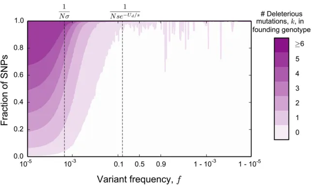
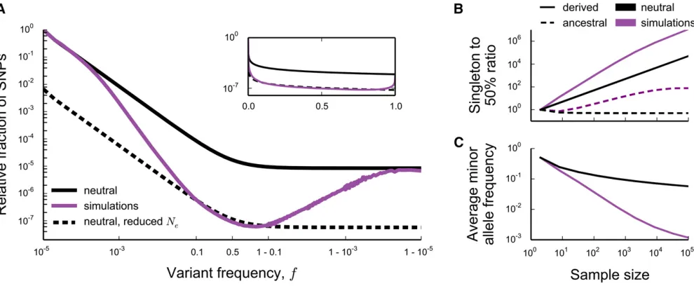
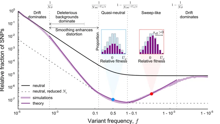
In Figure 1A, we show an example of the site frequency spectrum of neutral mutations at a locus experiencing strong background selection, generated by Wright–Fisher forward-time simulations. This example shows several key generic features of background selection. First, at intermediate fre-quencies the site frequency spectrum has a neutral shape,

pðfÞ}f21_; _{with the total number of such}

intermediate-frequency polymorphisms consistent with the simple reduced

“effective population size” prediction (Charlesworth et al.

1993). However, at both low and high frequencies, pðfÞ is signiﬁcantly distorted. At low frequencies, we see an enor-mous excess of rare alleles, qualitatively similar to what we expect in expanding populations (Slatkin and Hudson 1991; Rannala 1997). We also see a large excess of very high fre-quency variants, leading to a nonmonotonic site frefre-quency spectrum. This is reminiscent of the nonmonotonicity seen in the presence of positive selection (Sawyer and Hartl 1992). Notably, these distortions at both high and low frequencies arise in populations of constant size in which all variation is either neutral or deleterious.

The excess of rare derived alleles arises because selection takes aﬁnite amount of time to purge deleterious genotypes. Thus we expect that there can be substantial neutral variation linked to deleterious alleles that, although doomed to be

Figure 1 (A) The (unfolded) average site frequency spectrum of neutral alleles along a nonrecombining genomic segment experiencing strong background selection deviates strongly from the prediction of neutral theory. The purple line shows the simulated neutral site frequency spectrum in Wright–Fisher simulations of an asexual population ofN¼105_{individuals, where deleterious mutations occur at rate}_NU

d¼5000 and all have the

same effect onﬁtnessNs¼1000:The black lines show the neutral expectation for the site frequency spectrum of a population ofNandNe¼Ne2Ud=s

individuals (solid and dashed line, respectively). The inset shows the same data, but with thex-axis linearly scaled to emphasize intermediate frequencies. Simulated site frequency spectra were obtained by measuring whole-population neutral site frequency spectra in 105_Wright_–_{Fisher simulations, in} which neutral mutations were set to occur at rateNUn¼103;and by averaging and then smoothing the obtained curve using a box kernel smoother of

(4)

eventually purged from the population, can still reach modest frequencies. At the very lowest frequencies, we expect that neutral mutations arising in all individuals in the population (independent of the number of deleterious mutations they carry) can contribute. Thus, at the lowest frequencies, the site frequency spectrum should be unaffected by selection and should agree with the neutral site frequency spectrum of a population of sizeN. On the other hand, as argued above, the total number of common alleles must reﬂect the (much smaller) number of deleterious-mutation-free individuals, because only neutral mutations arising in such individuals can reach such high frequencies. Since the overall number of very rare alleles is proportional to the census population size N, and the number of common alleles reﬂects a much

smaller deleterious-mutation-free subpopulation, there must be a transition between these two: between these extremes the site frequency spectrum must fall off more rapidly than the neutral predictionpðfÞ f21_:_{This transition reﬂects the}

fact that as frequency increases, the effect of selection will be more strongly felt, and neutral mutations arising in geno-types of increasingly lowerﬁtnesses will become increasingly unlikely.

As the frequency increases even further, we see from our simulations that the total number of polymorphisms increases again until, at very high frequencies, it matches the prediction for a neutral population of size equal to the census sizeN. Note that, at these frequencies, the total number of backgrounds contributing to the diversity is constant (i.e., all mutations reaching these frequencies must arise in the small subpopu-lation of mutation-free individuals). This suggests that fun-damentally nonneutral behaviors must be dominating the dynamics of these high frequency neutral polymorphisms. To understand this, as well as the details of the rapid falloff at very low frequencies, we will need to develop a more de-tailed description of the trajectories of neutral alleles in the population; we analyze this in quantitative detail in a later section.

However, a simple argument can explain the agreement with the neutral prediction at the highest frequencies. Poly-morphisms observed at these very high frequencies corre-spond to neutral variants that have almost reachedfixation. The ancestral allele is still present in the population, but at a very low frequency. In principle, the dynamics of the derived and ancestral alleles should depend on thefitnesses of their backgrounds. However, once the frequency of the ancestral allele is sufficiently low, the effects of drift will once again dominate over the effects of selection. Thus, at extremely high frequencies of the derived allele, its dynamics must become neutral. In addition to having neutral dynamics, the overall rate at which neutral mutations enter this high-frequency regime also agrees with the rate in a neutral population at the census population size. This is because, at steady state, the total rate at which neutral mutationsfix is equal to the product of the rate at which they enter the population at any point in time (NUn) and their fixation probability, 1=N (Birky and Walsh 1988). Thus, since the total rate at which alleles enter

this high-frequency regime is unaffected by selection, and since their dynamics within this regime are neutral, we ex-pect that the site frequency sex-pectrum should also agree with the neutral prediction for a population of sizeN.

Although these simple arguments do not provide a full quantitative explanation of the site frequency spectrum, they already offer some intuition about the presence and magni-tude of the distortions due to background selection. First, these distortions arise in part as a result of the difference in the number of backgrounds on which mutations that remain at the lowest frequencies and mutations that reach substantial fre-quencies can arise. Thus, they will always occur when back-ground selection is strong enough to cause a substantial reduction in the effective population size: if the pairwise diversitypis at all reduced compared to the neutral expec-tation p0 [p=p0,1; or, in terms of McVicker’s B statistic,

B,1 (McVicker et al. 2009)], these distortions exist (see Figure 1A). Second, because the distortions from the neutral shape are limited to high and low ends of the frequency spectrum, they will have limited effect on site frequency spec-tra of small samples, but will have dramatic consequences as the sample size increases (see Figure 1, B and C). On a prac-tical level, this means that extrapolating conclusions from small samples about the effects of background selection can be grossly misleading.

Data availability

Code used to generate the simulated data are available at:

https://github.com/icvijovic/background-selection. Sup-plemental material available at Figshare:https://doi.org/ 10.25386/genetics.6167591.

Model and Results

In the next few sections, we will analyze the dynamics of neutral mutations under background selection in detail. We focus on the simplest possible model of purifying selection at a perfectly linked genetic locus in a population ofNindividuals. We assume neutral mutations occur at a locus, per-generation rateUnand deleterious mutations occur at rateUd

(5)

work (Good and Desai 2013; Neher and Hallatschek 2013; Good et al. 2014). In the Discussion, we comment on the connection between these earlier weak-selection results and the strong-selection case we study here.

Our model is equivalent to the nonepistatic case of the model formulated by Kimura and Maruyama (1966) and Haigh (1978) as well as to theh¼1=2 case of the model considered by Charlesworthet al. (1993) and Hudson and Kaplan (1994), and later studied by many other authors (Gordoet al.2002; Segeret al.2010; Nicolaisen and Desai 2012; Walczaket al.2012). However, instead of modeling the genealogies of a sample of individuals from the population backwards in time, we offer a forward-time analysis of this model in which we analyze the full frequency trajectory of alleles.

In the presence of strongly selected deleterious mutations (Nse2Ud=s_{1), we}ﬁnd that the magnitude of the effects of background selection critically depends on the ratio,l, of the deleterious mutation rate, Ud; to the selective cost of each deleterious mutation,s:l¼Ud=s(Figure 2). This ratio con-trols the overall variance in the number of deleterious muta-tions carried by individuals in the population, which is equal

to l¼Ud=s (Kimura and Maruyama 1966). Whenever

l1;both the overall genetic diversity and the full neutral site frequency spectrumpðfÞare unaffected by background selection and the site frequency spectrumpðfÞis to leading order equal to

pðfÞ 2NUn

f when l1: (1)

This prediction agrees with the results of forward-time sim-ulations (see Figure 2). The intuition behind this result is simple: in the limit thatl1;a majority of individuals in

the population are free of deleterious mutations; neutral al-leles are therefore rarely linked to deleterious mutations. This results in a neutral site frequency spectrum.

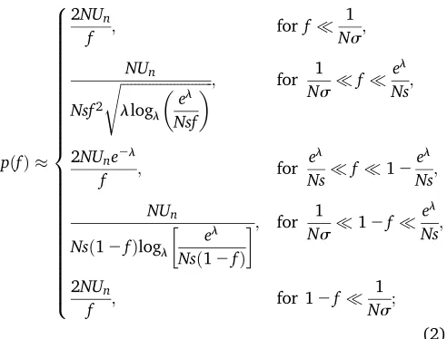
However, we will show that the site frequency spectrum of neutral mutations follows a very different form whenl1:

pðfÞ

2NUn

f ; for f

1

Ns;

NUn

Nsf2

ffiffiffiffiffiffiffiffiffiffiffiffiffiffiffiffiffiffiffiffiffiffiffiffiffiffi

llog_l

el

Nsf

s ; for 1

Nsf

el

Ns;

2NUne2l

f ; for

el

Nsf 12 el

Ns;

NUn

Nsð12fÞlog_l

el

Nsð12fÞ

; for 1

Ns12f

el

Ns;

2NUn

f ; for 12f

1

Ns;

8 > > > > > > > > > > > > > > > > > > > > > > > > > < > > > > > > > > > > > > > > > > > > > > > > > > > : (2)

wheres¼pffiffiffiffiffiffiffiUdsrepresents the standard deviation infitness in the population, and line 2 in Equation 2 is valid up to a constant factor (seeContribution from the Peaks of Trajecto-riesin Appendix I for details). Comparisons between Equa-tion 2 and simulaEqua-tions of the model are shown in Figure 2. We note thatpðfÞmatches the site frequency spectrum of a neutral population with a smaller effective population size

Ne¼Ne2l for 1=ðNse2lÞ,f,121=ðNse2lÞ; but deviates strongly outside this frequency range. This implies that sum-mary statistics based on the site frequency spectrum (e.g., the average minor allele frequency) will start to deviate from the

Figure 2 Comparison between the theoreti-cal predictions for the site frequency spectrum and Wright–Fisher simulations. In all simula-tions,Nse2Ud=s¼₁₀₀₀_e25₆:₇₃;_while

the parameterl¼Ud=svaries from 5 to

0.1 (values shown onﬁgure). Dashed lines show the expectations for a neutral pop-ulation at reduced effective poppop-ulation sizeNe¼Ne2l:At frequencies smaller

than 1=ðNsÞ (where s¼ ffiffiffiffiffiffiffiffiUds p

) and larger than 121=ðNsÞ; the theoretical predictions agree with the predictions for a neutral population with census size N(black line). Within the range 1=ðNsÞ,f,121=ðNsÞ; the theoreti-cal predictions (Equation 2) are given by colored lines. A single theory curve was constructed from Equation 2 by joining the piecewise forms using sigmoid func-tions (for details seeConstructing a Single Curve from Piecewise Asymptotic Functionsin Appendix I). Note that this involvesﬁttingOð1Þconstants to the curve, for reasons explained inContribution from the Peaks of TrajectoriesandConstructing a Single Curve from Piecewise Asymptotic Functionsin Appendix I. The values of the constants used are tabulated in Table I1. In simulations in whichl$1;N¼105_whereas_N_¼₁₀4_{for smaller}

l. In all simulations, the per-individual, per-generation neutral mutation rate isUn¼0:1 and site frequency spectra were obtained from these simulations as

(6)

neutral expectation in samples larger thanNse2l¼“Nes” in-dividuals, but not in smaller samples (Figure 1, B and C).

Our results also offer an intuitive interpretation of the origins of these distortions, which are summarized in Figure 3. When Uds;a large majority of individuals in the pop-ulation will carry some deleterious mutations at the locus, which results in substantialﬁtness variation within the pop-ulation. However, the majority of neutral alleles are pre-sent on backgrounds that are within OðsÞ of the mean of the distribution. Thus, at frequencies f 1=ðNsÞ and 12f1=ðNsÞ;the effects of genetic drift dominate over any effects of linked selection for the majority of neutral alleles. At these frequencies, the site frequency spectrum agrees with that of a neutral population of size N (see Figure 3).

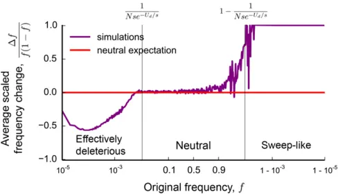
In contrast, the effects of linked selection have a crucial impact on allele frequency trajectories at frequencies f for which 1=ðNsÞ f 121=ðNsÞ:As we show in a later sec-tion, this region of the site frequency spectrum is dominated by alleles that arise on unusually ﬁt backgrounds [with ﬁt-ness with respect to the mean larger thanOðsÞ]. For these alleles, a crucial distinction arises between their short-term and long-term behavior: although genotypes that carryany

polymorphic strongly deleterious variants are guaranteed to be eventually purged from the population, those that contain

fewer than average deleterious mutations are still positively selected on shorter timescales. This results in strong nonneu-tral features in the frequency trajectories of these alleles. Their trajectories are characterized by rapid initial expan-sions, followed by a peak, and eventual exponential decline (Figure 4). These deterministic aspects of allele frequency

trajectories are similar to those seen by Neher and Shraiman (2011) in models of linked selection in large facultatively sexual populations. We describe them in detail in the section titled Key features of lineage trajectories. A part of the rapid falloff in the site frequency spectrum between f ¼1=ðNsÞ and f ¼1=ðNse2lÞ results from these deterministic effects: alleles arising on backgrounds with more deleterious variants can reach more limited frequencies than alleles arising on backgrounds with fewer deleterious variants. Thus, the num-ber of backgrounds on which neutral alleles could have arisen declines with the frequency, leading to a falloff of the site frequency spectrum.

However, these deterministic aspects of the allele quency trajectory are not sufficient to produce the site fre-quency spectrum in Equation 2, even if stochastic effects in the early phase of the trajectory are taken into account (i.e., dur-ing “establishment”; see Desai and Fisher 2007 and Neher and Shraiman 2011). This is becausefluctuations in the num-bers of most-fit individuals that occur after establishment continue to drivefluctuations in the overall allele frequency. This is closely related to the fluctuations in the population fitness distribution studied by Neher and Shraiman (2012) in an analysis of Muller’s ratchet.

In theAnalysis, we quantify how thesefluctuations prop-agate to shape the statistics of allele frequency trajectories, finding thatfluctuations in the number of most-fit individuals that happen on a timescale shorter than 1=sare smoothed out due to thefinite timescale on which selection can respond. In contrast,fluctuations that happen on timescales longer than 1=sare faithfully reproduced in the allele frequency tra-jectory, which leads to quasi-neutral statistics of allele

Figure 3 A summary of the dominant effects shaping the site frequency spec-trum. The site frequency spectrum and theoretical predictions are reproduced from Figure 1 and Figure 2 (l¼5). At frequencies below 1=ðNsÞ and above 121=ðNsÞ;the allele frequency trajecto-ries of the majority of neutral alleles are dominated by drift, resulting in neutral site frequency spectra corresponding to a population of sizeN. In contrast, linked selection has a crucial impact for 1=ðNsÞ,f,121=ðNsÞ:The rapid fall-off of the site frequency spectrum for 1=ðNsÞ,f,1=ðNse2l_Þ_{is primarily a}

re-sult of allele frequency trajectories having fundamentally nonneutral properties. In this regime, the number of backgrounds on which neutral alleles can arise also declines with the frequency f. As we show later, forf1=ðNUde2lÞ;the site

frequency spectrum is dominated by neutral mutations originating on deleterious backgrounds. In contrast to the rapid decline at lower frequencies, the site frequency spectrum has a neutral shape betweenf¼1=ðNse2l_Þ_and_f_¼₁₂₁₌_ð_Nse2l_Þ_:_{In this regime, both the neutral and wild-type allele are in approximate mutation}_–

selection balance (see blue dot and blue inset, showing thefitness distribution of such alleles) and largefluctuations of the allele frequency mirror the neutralfluctuations of the mostfit individuals. At frequencies larger than 121=ðNse2l_Þ_;_{the relative number of polymorphisms increases with the}

(7)

frequency trajectories at frequencies between 1=ðNse2lÞ

and 121=ðNse2lÞ(see Figure 3). The smoothing of ﬂuctu-ations on aﬁnite timescale introduces an additional funda-mentally nonneutral feature in the total allele frequency trajectory. This distorts the site frequency spectrum at fre-quencies below 1=ðNse2lÞabove and beyond what would be predicted if we asserted a simple frequency-dependent ef-fective population size equal to the number of backgrounds that can contribute to a given frequency.

Finally, we will demonstrate that the nonmonotonicity in the site frequency spectrum at frequencies between 121=ðNse2lÞand 121=ðNsÞarises as a result of sweep-like behaviors of neutral alleles that havefixed among the most-fit individuals in the population (see Figure 3). Because these derived alleles carry, on average, fewer deleterious mutations than the wild type, they are positively selected despite having no inherent benefit. We will show that this difference in the average number of linked deleterious mutations gives rise to an effective frequency-dependent selection coefficientseffðfÞ:

This selection coefﬁcient changes with the frequencyfof the mutation as high-ﬁtness, wild-type individuals ratchet to extinction:

seffðfÞ ¼logl

1

Nse2l_ð1₂_f_Þ

s;

if 12f 1 Nse2l:

(3)

In the next sections, we derive the form of the site frequency spectrum in Equation 2 and explain these effects in more detail. We begin by presenting background necessary for understanding these results. We ﬁrst revisit the intuition behind the shape of the site frequency spectra of isolated loci (Ewens 1963; Sawyer and Hartl 1992). We show that, in the absence of linkage between multiple selected sites, back-ground selection does not lead to a site frequency spectrum of the form in Equation 2. Next, we explain how linkage be-tween multiple selected sites modiﬁes allele frequency tra-jectories. We revisit the key deterministic aspects of allele frequency trajectories in the presence of background selec-tion, previously studied by Etheridgeet al.(2009) and others, and extend these results to identify the key timescales impor-tant for understanding this problem. Finally, we turn to a full stochastic treatment of allele frequency trajectories in the

Analysis, where we also derive the expressions for the site frequency spectra of neutral and deleterious mutations. In theDiscussion, we comment on the practical implications of our results, as well as on connections to previous work and other models.

Background

Isolated loci

To gain insight into the more complicated case of linked selection, weﬁrst begin by reviewing the simplest case of a

single locus isolated from any other selected loci. The prob-ability that an allele at that locus is present at frequencyfat timet,pðf;tÞ;is described by the diffusion equation:

@p

@t¼ 2

@ @f

h

sfð12fÞpiþ @

@f2

fð12fÞ

2N p

: (4)

Ewens (1963) showed that the expected site frequency spec-trum can be obtained from this forward-time description of the allele frequency trajectory: because mutations are arising uniformly in time and the time at which a mutation is ob-served is random, the site frequency spectrum is proportional to the average time an allele is expected to spend in a given frequency window.

In this section, we show that the low- and high-frequency ends of the site frequency spectrum of isolated loci can be obtained from a simple heuristic argument that emphasizes this connection between allele frequency trajectories and the site frequency spectrum. These calculations are not intended to be exact [resulting frequency spectra are only valid up to Oð1Þfactors], but they provide intuition for the origins of key features of the site frequency spectrum that we will return to more formally below.

Consider the simplest case of isolated, purely neutral loci. Neutral mutations will arise in the population at rateNUn:In the absence of selection, the trajectories of these mutations are governed by genetic drift. At steady state, the number of mutations we expect to see at frequencyfis simply propor-tional to the number of mutations that reach that frequency and the typical time each of these mutations spends at that frequency before ﬁxing or going extinct. In the absence of selection, a new mutation that arises at initial frequency

f0¼1=N will reach frequency f before going extinct with

probabilityf0=f ¼1=ðNfÞ:Standard branching process

calcu-lations (Fisher 2007) show that, given that it reaches fre-quency f, the mutation will spend about Nf generations around that frequency [deﬁned as logðfÞ not changing by more thanOð1Þ], provided thatfis small (f1).

By combining these results, we can calculate the expected site frequency spectrum for smallf. The rate at which new muta-tions reach frequencyfisNUn1=ðNfÞ:Those that do will re-main around f (in the sense deﬁned above) for about Nf

generations. Thus the total number of neutral mutations within

df of frequency f is pðfÞdf NUn1=ðNfÞ NfdðlogfÞ: In other words, we have

pðfÞ NUn

f : (5)

(8)

withinOð1Þof logð12fÞ]. This givespðfÞ NUn=f NUnin the high-frequency end of the spectrum. This simple forward-time heuristic argument reproduces a well-known result of coalescent theory (Wakeley 2009) and agrees with the more formal calculation of sojourn times in the Wright–Fisher pro-cess (Ewens 1963).

We can use a similar argument to calculate the frequency spectrum of strongly selected deleterious mutations with ﬁtness effect2s(withNs1) that occur at a locus that is isolated from any other selected locus. Provided that the del-eterious mutation is rare (below the“drift barrier”frequency,

f,1=ðNsÞ), its trajectory is dominated by drift. Thus for f,1=ðNsÞ;the mutation trajectory will be the same as for a neutral mutation and the frequency spectrum will therefore be neutral. In contrast, at frequencies larger than 1=ðNsÞ;

selection is stronger than drift, which prevents the mutation from exceeding this frequency. Combining these two expres-sions, we ﬁnd that the frequency spectrum of an isolated deleterious mutation is, to a rough approximation, given by

pðfÞ NUd

f if f,

1

Ns

0 otherwise:

8 > < >

: (6)

For completeness, we also show how a similar argument can be used to obtain the frequency spectrum of beneficial muta-tions. Although it is not immediately obvious that this is relevant to background selection, we will later see how similar trajectories emerge in the case of strong purifying selection. Just like deleterious alleles, strongly beneficial alleles with fitness effects(withNs1) will not feel the effects of se-lection as long as they do not exceed the drift barrier (f,1=ðNsÞ). Their trajectory and frequency spectrum will

therefore be neutral below the drift barrier. As a result, only a small fraction s of beneﬁcial mutations will reach

fre-quency 1=ðNsÞ:However, those that do will be destined to ﬁx since, at frequencies larger than 1=ðNsÞ;selection domi-nates over drift. Above this threshold, selection will cause the

frequency of the mutation to grow logistically at rate s

[df=dt¼sfð12fÞ], spending 1=½sfð12fÞ generations near frequencyf. This is valid as long asf,121=ðNsÞ;at which point the effects of drift become dominant due to the wild type being rare, and the trajectory of the mutant is once again the same as the trajectory of a neutral mutation. Combining these expressions, we obtain a rough approximation for the fre-quency spectrum of an isolated beneﬁcial mutation:

pðfÞ NUb

f ; if f,

1

Ns NUb

fð12fÞ; if

1

Ns,f,12

1

Ns

NUbNs; if f.12 1

Ns: 8

> > > > > > > < > > > > > > > :

(7)

Linked loci under background selection

We now turn to the analysis of background selection. Since we assume that all mutations have the same effect onfitness, the population can be partitioned into discrete fitness classes according to the number of deleterious mutations each indi-vidual carries at the locus. When the fitness effect of each mutation is sufficiently strong, the population assumes a steady-statefitness distribution in which the expected frac-tion of individuals withkdeleterious mutations,hk;follows a Poisson distribution with mean k¼l (Kimura and Maruyama 1966; Haigh 1978):

hk¼e2ll k

k!: (8)

A new allele in such a population will arise on a background withkexisting mutations with probabilityhk:

From the form ofhkwe see that, depending on the value of

l, the population can be in one of two regimes. In theﬁrst regime, the rate at which mutations are generated is smaller than the rate at which selection can purge them (l1). In

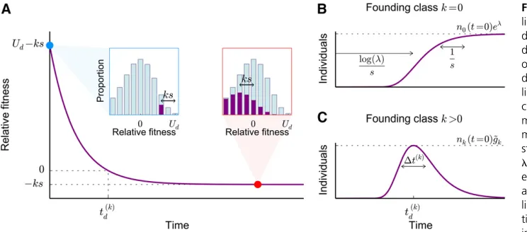
Figure 4(A) The average fitness of a lineage comprising individuals carryingk deleterious mutations at timet¼0 (blue dot and blue inset). As the descendants of these individuals accumulate further deleterious mutations, thefitness of the lineage declines until the individuals ac-cumulate an average of l deleterious mutations (red dot) and reach their own mutation–selection balance, which is a steady-state Poisson profile with mean lthat has been shifted by the initial del-eterious load,2ks;(red inset). (B) In the absence of genetic drift, the size of the lineage will increase at a rate propor-tional to its relativefitness. Lineages aris-ing in the class withk¼0 deleterious mutations reach mutation–selection balance abouttd¼logðlÞ=safter arising, after which the size of the lineage asymptotes ton0ðt¼0Þel: The

(9)

this case, the majority of individuals in the population carry no deleterious mutations (h01), with only a small

propor-tion, 12h0l;of backgrounds in the population carrying

some deleterious variants. To leading order in l, all new neutral mutations will arise in a mutation-free background and will remain at the sameﬁtness as the founding genotype. Their trajectories are thus the same as the trajectories of mutants at isolated genetic loci of the same ﬁtness as the founding genotype (see Appendix D for details). This means that the full site frequency spectrum can be calculated by summing the contributions of site frequency spectra of iso-lated loci that we calcuiso-lated above. The neutral and delete-rious site frequency spectra are, to leading order inl, given by Equations 5 and 6, respectively (see Appendix H for de-tails). Thus, background selection has a negligible impact on mutational trajectories and diversity whenl1:

In the opposite regime wherel1;mutations are gen-erated faster than selection can purge them and there will be substantialfitness variation at the locus. Consider a new allele (i.e., a new mutation at some site within the locus) that arises in this population. A short time after arising, individuals that carry this allele will accumulate newer del-eterious mutations, which will lead the allele to spread through thefitness distribution. The fundamental difficulty in calculating the frequency trajectory of this allele, fðtÞ;

stems from the fact that a short time after arising, individ-uals that carry the allele will have accumulated different numbers of newer deleterious mutations. The total strength of selection against the allele depends on the average num-ber of deleterious mutations that the individuals that carry the allele have. This will change over time in a complicated stochastic way as the lineage purges old deleterious muta-tions, accumulates new ones, and changes in frequency due to drift and selection. To calculate the distribution of allele frequency trajectories in this regime, we will need to model these changes in theﬁtness distribution of individuals car-rying the allele. Although we will formally be treatinglas a large parameter, in practice our results will also adequately describe allele frequency trajectories in the cases of moder-atel(i.e.,l*2;see Figure 2).

To make progress, we classify individuals carrying this allele (the “labeled lineage”) according to the number of deleterious mutants they have at the locus. We denote the total frequency of the labeled individuals that havei delete-rious mutations as fiðtÞ; so that the total frequency of the lineage,fðtÞ;is given by

fðtÞ ¼X

i

fiðtÞ: (9)

The time evolution of the allele frequency in a Wright–Fisher process is commonly described by a diffusion equation for the probability density of the allele frequency (Ewens 2004). Instead, for our purposes, it will be more convenient to consider the equivalent Langevin equation (Van Kampen 2007):

dfi

dt¼

2isþkðtÞsfi2UdfiþUdfi21þCiðtÞ: (10)

Here, CiðtÞ is a noise term with a complicated correlation structure that is necessary to keep the total size of the pop-ulationﬁxed (see Good and Desai 2013 for details), andkðtÞ

is the mean number of mutations per individual in the entire population at timet. In the strong selection limit that we are interested in here (Nse2l1),ﬂuctuations in the mean of the ﬁtness distribution of the population are small and

kðtÞ l(Neher and Shraiman 2012).

Key features of lineage trajectories

Before turning to a detailed analysis of Equation 10, it is helpful to consider some of the key features of lineage trajec-tories that we will model more formally below. To begin, imagine a lineage founded by a neutral mutation in an indi-vidual withkdeleterious mutations. Let the lineage comprise

nkð0Þindividuals at some timet¼0 shortly after arising, all of which carry k deleterious mutations (see blue inset in Figure 4A). At this time, the relative ﬁtness of this lineage is simply2ks2ð2ksÞ ¼Ud2ks:Thus, lineages founded in classes withk.lwill tend to decline in size. In contrast, the more interesting case arises ifk,l;since these lineages will tend to increase in size.

However, although the overall number of individuals that carry the allele will tend to increase whenk,l;the part of the lineage in the founding classk(the“founding genotype”) will tend to decline in size because it loses individuals through new deleterious mutations (at per-individual rate2Ud). As a result, the founding genotype feels an effective selection pressure of Ud2ks2Ud¼ 2ks; which is negative for all

k.0 and 0 fork¼0:This means that the lineage will in-crease in frequency, not through an inin-crease in size of the founding genotype, but rather through the appearance of a large number of deleterious descendants in classes of lower ﬁtness. The lineage must therefore decline in ﬁtness as it increases in size.

In the absence of genetic drift, we can calculate how the size andﬁtness of the lineage change in time by dropping the stochastic terms in Equation 10 [subject to the initial condition

nkðt¼0Þ ¼nkð0Þ and nkþiðt¼0Þ ¼0 for all i6¼0]. These

deterministic dynamics of the lineage have been analyzed previously by Etheridgeet al.(2009), who showed that the number of additional mutations that an individual in the lineage carries at some later timetis Poisson distributed with mean lð12e2st_Þ_: _{Thus the average number of}

addi-tional deleterious mutations eventually approacheslafter

t*td¼logðlÞ=sgenerations. At this point, the lineage has reached its own mutation–selection balance: theﬁtness dis-tribution of the lineage has the same shape as the distribu-tion of the populadistribu-tion [i.e.,niþkðtÞ ¼hinkðtÞ] but is shifted

by2kscompared to the distribution of the population (see red inset in Figure 4A).

(10)

xðtÞ ¼Ude2st2ks; (11)

and the total number of individuals in the lineage is

sim-plynðtÞ ¼nkðt¼0Þe Rt

0xðt9Þdt9[nkðt¼0ÞgkðtÞ;where we have

deﬁned

gkðtÞ ¼e2kstþlð12e 2st_Þ

: (12)

Thus, we can see from Equations 11 and 12 that lineages founded in the 0-class will, on average, steadily increase in size at a declining rate until they asymptote at a total size equal to

nkðt¼0Þel _roughly_td_¼_logð_l_Þ₌_s_{generations later (see}

Fig-ure 4B). In contrast, lineages founded in thek-class will in-crease in size for only

tð_dkÞ¼logðl=kÞ

s (13)

generations, when they peak at a size ofnkðt¼0Þ ~gk indi-viduals (see Figure 4C), where we have deﬁned

~ gk[el

k el

k

: (14)

The lineages remain near this peak size for about

DtðkÞ¼ 1ffiffiffi k

p

s (15)

generations (Figure 4C). At longer times, they exponentially decline at rate2ks(Figure 4C).

These simple deterministic calculations capture the aver-age behavior of an allele and show that all alleles founded in classes withk.0 are likely to be extinct on timescales much longer thantð_dkÞ;whereas sufﬁciently large lineages founded in

the 0-class should simply reﬂect the frequency in the founding class about td generations earlier: hfðtÞi el_f

0ðt2tdÞ: This

is the forward-time analog of the intuition presented by Charlesworthet al.(1993).

Of course, this deterministic solution neglects the effects of genetic drift, which will be crucial, particularly because drift in each class propagates to affect the frequency of the lineage in all lower fitness classes (for a more detailed heuristic de-scribing why drift can never be ignored, seeThe Importance of Genetic Drift in the Founding Classin Appendix B). Although these effects are complex, there is a hierarchy in the fluctua-tion terms which we can exploit to gain some intuifluctua-tion. From the deterministic solution above, we can see that a fluctua-tion of sizedfiin classiwill, on average, eventually cause a change in the total size of the lineage proportional to dfi~gi

after a time delay tdðiÞ:Thus, theﬂuctuations that have the

largest effect on the total size of the lineage are those that occur in the class of highestfitness (i.e., the founding classk). Thesefluctuations will turn out to be the most important in describing the frequency trajectory of the entire allele, al-thoughfluctuations in classes of lowerfitness will still matter in lineages of a small enough size.

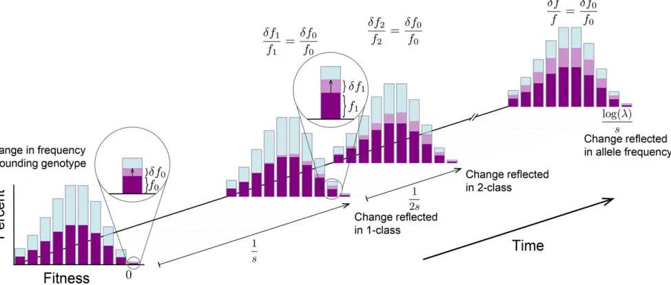
One could imagine that this result means thatfluctuations in the total size of the lineage simply mirror thefluctuations in the founding class, amplified by a factor~gkand after a time delayt_dðkÞ:Iffluctuations in the founding class are sufficiently slow, this is indeed the case. However, this is not true for fluctuations that occur on shorter timescales. Consider, for example, the case where a neutral mutation is founded in the mutation-free (k¼0) class. Imagine that the frequency of the allele in the founding class changes by a small amount fromf0 tof0þdf0 as a result of genetic drift (shown in the

ﬁrst panel of Figure 5). Based on the deterministic solution, thisﬂuctuation will lead to a proportional change in the fre-quency of the portion of the lineage in the 1-class, and this change will take place over1=sgenerations (see Appendix A for details). During this time, the change in the 1-class begins to lead to a shift in the frequency in the 2-class, which will mirror the change in the 0-class a further 1=ð2sÞ gener-ations later (see Figure 5). This change will then propa-gate, in turn, to lower classes and ultimately results in a proportional change in the total allele frequency a total of

Pl

i¼11=ðisÞ ¼logðlÞ=sgenerations later (see Figure 5).

Now consider what happens if there is another change in the frequency in the founding class. If this change occurs within the initial 1=s generations, it will inﬂuence the

1-class simultaneously with the first fluctuation, and thus the effect of these two fluctuations on the overall lineage frequency will be“smoothed”out. In contrast, if the changes are separated by more than 1=sgenerations, they will prop-agate sequentially through the fitness distribution and are ultimately mirrored in the total allele frequency. Similar ar-guments apply to lineages founded in otherfitness classes, though the relevant timescales and scale of amplification are different.

Together, these arguments suggest thatfluctuations in the founding class will have the largest impact on overall fluctu-ations in the lineage frequency, and these overallfluctuations will represent an amplified but smoothed-out mirror of the fluctuations in the founding class. This smoothing will be crucial: the size of the lineage in the founding class will typically fluctuate neutrally, but the smoothed-out and am-plified versions will have nonneutral statistics. As we will see below, this smoothing ultimately leads to distortions in the site frequency spectrum at low frequencies (f 1=ðNse2lÞ).

Analysis

(11)

by considering low-, high-, and intermediate-frequency lineages separately. First, at sufﬁciently low frequencies (f1), theCiðtÞin Equation 10 reduce to simple uncorre-lated white noise. At these low frequencies, Equation 10 thus simpliﬁes to

dfi

dt ¼ ð2isþlsÞfi2UdfiþUdfi21þ ffiffiffiffi fi

N r

hiðtÞ; (16)

where the noise terms have hhiðtÞi ¼0 and covariances

hhiðtÞhjðt9Þi ¼dijdðt2t9Þ and should be interpreted in the

Itô sense. At very high frequencies (12f 1), a similar sim-pliﬁcation arises. In this case, the wild-type lineage is at low frequency and we can model the wild-type frequency using an analogous coupled branching process with uncorrelated white noise terms. Finally, at intermediate frequencies, we cannot simplify the noise terms in this way. Fortunately, for the case of strong selection we consider here, we will show that for 1=ðNse2lÞ f 121=ðNse2lÞ;lineage trajectories have neu-tral statistics on relevant timescales. As we will see below, these low-, intermediate-, and high-frequency solutions can then be asymptotically matched, giving us allele frequency trajectories and site frequency spectra at all frequencies.

In the next several subsections, we focus on the analysis of the distribution of trajectories at low and high frequencies (f1 or 12f 1), where Equation 16 is valid. We then return in a later subsection to the analysis of trajectories at intermediate frequencies.

The dynamics of the lineage within eachﬁtness class

To obtain the distribution of trajectories of the allelepðf;tÞ

at low frequencies (f 1) from Equation 16, we willﬁrst

compute the generating function of fðtÞ: This generating function is deﬁned as

Hfðz;tÞ ¼

D e2zfðtÞ

E

; (17)

where angle brackets denote the expectation over the prob-ability distribution of the frequency trajectoryfðtÞ:Hfðz;tÞis simply the Laplace transform of the probability distribution of

fðtÞand it therefore contains all of the relevant information about the probability distribution offðtÞ:

As we have already anticipated from our discussion above, the time evolution offðtÞdepends on the distribution of the lineage among differentﬁtness classes. To understand how this distribution changes under the inﬂuence of drift, muta-tion, and selection in these classes, we can consider the joint generating function for thefiðtÞ;

Hðfzig;tÞ ¼

D e2

P

izifiðtÞ

E

: (18)

The generating function for the total allele frequencyHfðz;tÞ

can then be obtained from this joint generating function by settingzi¼z:We will use this relationship between the two generating functions to evaluate the importance of drift, mu-tation, and selection within each of theﬁtness classes on the total allele frequency.

By taking a time derivative of Equation 18 and substitut-ing the time derivativesdfi=dtfrom Equation 16 (where the stochastic terms should be interpreted in the Itô sense, see Appendix C), we can obtain a partial differential equation (PDE) describing the evolution of the joint generating function:

Figure 5 A schematic showing how a change in the frequency of the lineage in the mutation-free class propagates to affect the frequency in all classes of lowerﬁtness. At timet¼0;the lineage is in mutation–selection balance at total frequencyf, when the frequency of the portion of the lineage in the 0-class changes suddenly fromf0tof0þdf0:This change is felt in the 1-class 1=sgenerations later and propagates to the 2-class yet another 1=ð2sÞ generations later. The lineage reaches a new equilibrium about logðlÞ=s generations later, when the total allele frequency is proportional to

(12)

@H

@t ¼ X

i 2

iszi2Udziþ1þ

z2_i

2N

@H

@zi:

(19)

We see from Equation 19 that the joint generating function is constant along the characteristicsziðt2t9Þdeﬁned by

dzi

dt9¼is zi2Udziþ1þ z2_i

2N: (20)

Thus, the joint generating function can be obtained by in-tegrating along the characteristic backward in time from

t9¼0 tot9¼t;subject to the boundary conditionziðtÞ ¼z:

Note that the linear terms in the characteristic equations arise from selection and mutation out of the i-class and that the nonlinear term arises from drift in classi.

InLarge Lineages Arising on Unusually Fit Backgroundsin Appendix E, we show that when considering the distribu-tion of trajectories pðf;tÞ at frequencies f el_½_i₌_ð_e_lÞi

= ð2NsiÞ ¼~gi=ð2NsiÞ the nonlinear terms in Equation 20 are of negligible magnitude uniformly in time in all classes con-taining i or more deleterious mutations per individual, as long as il; Nse2l 1; and l1: Here, ~gi represents

the peak of the expected number of individuals in a lineage founded by a single individual in classi(see Equation 14 and Figure 4C). Thus, whenf~gi=ð2NsiÞ;the effect of genetic drift is negligible in classes withior more deleterious mutations. Conversely, whenf ~gi=ð2NsiÞ;genetic drift in the class withi

deleterious mutations does affect the overall allele frequency. Since drift is negligible in classes withior more mutations, total allele frequencies of fðtÞ ~gi=ð2NsiÞ require that

fi t2tðdiÞ

1=ð2NsiÞ:This threshold is reminiscent of the

drift barrier, but its origin for classes below the founding class (i.k) is more subtle. We offer an intuitive explanation for this threshold in The Importance of Genetic Drift in Classes Below the Founding Classin Appendix B. Thus, drift in class

ihas an important impact on the overall frequency trajectory as long asfi1=ð2NsiÞ:However, oncefiexceeds 1=ð2NsiÞ;

the effect of genetic drift in that class, as well as in all classes belowi, becomes negligible because the frequencies of the parts of the lineage in all classes belowiare then also guaranteed to exceed the corresponding thresholds. Note that the frequency of the founding genotypefkis exponentially unlikely to substan-tially exceed 1=ð2NskÞ:This is because, as we explained earlier, the frequency trajectory of the founding genotypefkðtÞhas the same statistics as the trajectory of a mutation ofﬁtness2ksat an isolated locus (see Equation 16 and Appendix F). Thus, because

fkis unlikely to exceed 1=ð2NskÞ;the overall allele frequencyf

of an allele founded in class k is exponentially unlikely to substantially exceed~gk1=ð2NskÞ.

In summary, by analyzing the generating function for the components of the lineage in differentfitness classes, we have found that there is a clear separation between high-fitness classes in which mutation and drift are the primary forces, and classes of lower relative fitness in which mutation and selection dominate. The boundary between the stochastic and

deterministic classes can be determined from the total allele frequency, allowing us to reduce a complicated problem in-volving a large number of coupled stochastic terms to what we will see is a small number of stochastic terms feeding an otherwise deterministic population.

Statistics of trajectories withg~₁=ð2NsÞf1

At this point, we are in a position to calculate a piecewise form for the generating functionHfðz;tÞ;valid near any frequency

f. For example, consider the allele frequency trajectory in the vicinity of some frequency ~g1=ð2NsÞ f 1:As we have

explained above, at these frequencies contributions from mu-tations arising in classk$1 are exponentially small, since they would require the frequency of the lineage in that class to sub-stantially exceed 1=ð2NsÞ; which happens only exponentially rarely. Thus, in this frequency range we will only see mutations arising in the mutation-free class (k¼0). In addition to this, we have shown that at these frequencies genetic drift can be neglected in all classes but the 0-class. To obtain the generating function at these frequencies, we can therefore integrate the characteristic equations by dropping the nonlinear terms in Equation 20 for alli.0 [seeLarge Lineages Arising on Unusually Fit Backgroundsin Appendix E for details]. This yields the gen-erating function for the frequency of the labeled lineage:

Hfðz;tÞ ¼

* e2z

f0þUd

Rt

2Ndtf0ðtÞg1ðt2tÞ +

; (21)

where the average is taken over all possible realizations of the trajectory in the founding classf0ðtÞ:

As before, g1ðt2tÞ represents the expected number of

individuals descended from an individual present in the 1-class t2t generations earlier (see Equation 12). Thus, the two terms in the exponent in Equation 21 represent the frequency of the lineage in the founding classf0and the total

frequency of the deleterious descendants of that lineage. The latter are seeded into the 1-class at rateNUdf0ðtÞand each of

these deleterious descendants founds a lineage that t2t generations later contains g1ðt2tÞ individuals, so that the

total frequency of the allele is simply

fðtÞ ¼f0ðtÞ þUd

Z t

2Ndtf0ðtÞg1ðt2tÞ: (22)

Thus, we have obtained a simple expression for the frequency of the entire allele in which all of the stochastic effects have been reduced to a single stochastic component,f0ðtÞ:

Further-more, the stochastic dynamics off0ðtÞare those of a simple,

isolated, neutral mutation (see schematic of such a trajectory in Figure 6B). Note, however, that the statistics of the ﬂuctua-tions infðtÞare not necessarily the same as the statistics of the trajectory in the founding class (see Figure 6A). This is because

fðtÞdepends on anintegraloff0ðtÞ(see Equation 22) and

there-fore has different stochastic properties thanf0ðtÞitself.

(13)

have seen in the deterministic behavior of mutations. Shortly after being founded, the lineage will become dominated by the deleterious descendants of the founding class, which are captured by the second term in Equation 22 (see left inset in Figure 6A). At early times [ttd¼logðlÞ=s], the total allele frequency must rapidly grow as the lineage spreads through the fitness distribution and approaches mutation– selection balance (see Figure 6A). Abouttdgenerations after founding, the peak phase of the trajectory begins (see Figure 6A). During this phase, the averagefitness of the lineage is approximately zero and the allele traces out a smoothed-out and amplified version of the trajectory in the founding class (Figure 6B). Finally,tdgenerations after the descendants of the last individuals present in the founding class have peaked, the averagefitness of the lineage will fall significantly below zero and the extinction phase of the trajectory begins.

As we show in Appendix I, the peak phase of the trajectory is the most important for understanding the site frequency spectrum. This is also the phase during which the trajectory of the mutation spends the longest time near a given fre-quency. In contrast, the spreading phase (see Figure 6A) has a negligible effect on the site frequency spectrum: by this we mean that the site frequency spectrum at a given frequency will always be dominated by the peak phase of trajectories that peak around that frequency, and will not be inﬂuenced by the spreading phase of trajectories that peak at much higher frequencies. We will therefore not consider the spread-ing phase in the main text, but discuss it inContribution from the Spreading Stage of Trajectories in Appendix I. The extinction phase of the trajectory can also be neglected for a similar rea-son, except when considering the very highest frequencies:

f 121=ðNse2lÞ(seeContribution from the Extinction Stage of Trajectoriesin Appendix I). At these frequencies, the wild-type frequency is small and the mutant is in the process ofﬁxation. To analyze the allele frequency trajectory at these frequencies, we model the wild type using the coupled branching process in Equation 16 and hence describe these trajectories by the extinc-tion phase of the wild type.

To calculate the distribution offðtÞin the peak phase, we need to calculate the distribution of the time integral off0ðtÞ

in Equation 22. We can simplify this integral by observing that g1ðtÞ is highly peaked in time between tð1Þ_d 2Dtð1Þ=2

andtð1Þ_d þDtð1Þ=2;wheretð1Þ_d andDtð1Þare given by Equations 13 and 15 and are annotated in Figure 4C. In other words, starting at times around tdð1Þ generations after the lineage

reaches a substantial frequency in the founding class, the labeled lineage is dominated by the deleterious descen-dants of individuals extant in the founding class between

tð1Þ_d 2Dtð1Þ=2 andtð1Þ_d þDtð1Þ=2 generations earlier, with indi-viduals extant in the founding class at other times having exponentially smaller contributions [seeLarge Lineages Aris-ing on Unusually Fit Backgroundsin Appendix E for details]. Thus, the total size of the lineage will be proportional not to the frequencyf0 t2tð1Þ_d

in the founding classt_dð1Þgenerations

earlier, but to the total time-integrated frequency within some

window of widthDtð1Þcentered around that time. We call this quantity the“weight”and denote it byW_Dtð1Þ;where

W_Dtð1ÞðtÞ ¼

Z tþDtð1Þ

2

t2Dtð1Þ

2 f0 t9

dt9: (23)

The total allele frequency in the peak phase is therefore equal to

fðtÞ UdWDtð1Þðt2tdÞg1ðtdÞ: (24)

Thus, to calculate the distribution of the allele trajectory, we only need to calculate the distribution of the weight in the founding class over a window of speciﬁed width,Dtð1Þ:It is informative to consider the time-integrated form of the dis-tribution of this weight,pðWDtð1ÞÞ ¼

R_N

2Ndt pðWDtð1Þ;tÞ;since this form is also directly relevant to the site frequency spec-trum [for a discussion of the time-dependent distribution

W_Dtð1ÞðtÞ; see Appendix F]. In Appendix F we show that

pðW_Dtð1ÞÞis given by

(14)

pðW_Dtð1ÞÞ 1

ffiffiffiffiffiffiffiffiffiffi

2Np p Dtð1Þ

W_D3=_tð21Þ

; W_Dtð1Þ Dt ð1Þ2

N ;

1

W_D_tð1Þ; WDt ð1Þ Dt

ð1Þ2

N : 8 > > > > > < > > > > > : (25)

This distribution has a form that can be simply understood in terms of the trajectory in the founding class. Since genetic drift takes orderNf0 generations to changef0 substantially,

drift will not change f0 signiﬁcantly within Dtð1Þ

genera-tions when the frequency in the founding class exceeds

Dtð1Þ=N¼1=ðNsÞ:As a result, the weight,W_Dtð1Þ;will be ap-proximately equal to W_Dtð1Þf0Dtð1Þ¼f0=s:Therefore, at

these large frequencies, the weight simply traces the found-ing class frequency and the two quantities have the same distributions. At lower frequencies, f01=s; the founding

genotype will typically have arisen and gone extinct in a time of orderNf0;maxgenerations (wheref0;maxis the maximal

fre-quency the lineage reaches over the course of its lifetime). By assumption, this time is much shorter than 1=s: Thus, the weight in a window of width 1=sthat contains this trajectory is simply W_Dtð1Þ¼f0;maxNf0;max: This large a trajectory is

obtained with probability 1=ðNf0;maxÞ;from which it follows

(by a change of variable) that the distribution of weights in the founding class scales asW_D23_tð1=Þ2:

As we anticipated in our discussion of the propagation of fluctuations of the founding genotype through the fitness distribution (Figure 5), we have found that the trajectory of the allele in the peak phase looks like a smoothed-out, time-delayed, and amplified version of the trajectory in the founding class (Figure 6). At sufficiently high frequencies,

fðtÞ U~g11=ðNs2Þ 1=ðNse2lÞ;the timescale of the

smooth-ing is shorter than the typical timescale of thefluctuations in the founding class. At these frequencies, the statistics of the fluctuations of the allele simply mirror the statistics of the fluctuations in the founding class, with a time delay equal to

tð1Þ_d ¼logðlÞ=s:

At lower frequencies, ~g1=ð2NsÞ f1=ðNse2lÞ; the

timescale of smoothing is much longer than the typical life-time of the founding genotype. As a result, the deleterious descendants of the entire original genotype rise and fall si-multaneously andﬂuctuations in the founding class are not reproduced in detail. Instead, the peak phase of the allele frequency trajectory consists of a single peak with size proportional to the total lifetime weight of the founding genotype,W¼R₂N_NfðtÞdt:As we calculated above, the dis-tribution of these peak sizes falls off more rapidly than neu-trally. This gives us a complete description of the statistics of the peaks of allele frequency trajectories in the frequency rangef ~g1=ð2NsÞ:

Statistics of trajectories with f~g₁=ð2NsÞ

So far, we have only considered trajectories of lineages that reach a maximal allele frequency larger than~g1=ð2NsÞ;all of

which must have arisen in the mutation-free class. At lower

frequencies,~g2=ð4NsÞ f ~g1=ð2NsÞ;the effects of genetic

drift in classi¼1 must also considered, but the behavior in classes withi$2 is deterministic. In this case, by repeating our earlier procedure, we obtain a slightly different form for the generating functionHfðz;tÞ;

Hfðz;tÞ ¼

e2z

f0þf1þUd

Rt

2Ndtf1ðtÞg2ðt2tÞ

; (26)

so that the total allele frequency is

fðtÞ ¼f0ðtÞ þf1ðtÞ þUd

Z t

2Ndtf1ðtÞg2ðt2tÞ: (27)

The total allele frequency is once again dominated by the last term, which represents the bulk of the deleterious descen-dants. Thus, by an analogous argument, the peak size of the lineage is proportional to the weight in the 1-class in a window of widthDtð2Þ¼1=ðpffiffiffi2sÞ:

fðtÞ UdWDtð2Þ t2tð_d2Þ

~

g2: (28)

There are two types of trajectories that can reach these frequencies: trajectories that arise in the 1-class and reach a sufﬁciently large frequency in their founding class (f1 l1=2=ð

ffiffiffi

2 p

NUdÞ;see Appendix G); and trajectories that arise in the 0-class and reach a smaller frequency in their founding class (f0l1=2=ð

ffiffiffi

2 p

NUdÞ), but still leave behind

enough deleterious descendants in the 1-class that the overall frequency in that class exceeds f1l1=2=ð

ffiffiffi

2 p

NUdÞ:By the argument that we outlined before, this ensures that genetic drift will negligible in classes of lower ﬁtness (i.e., for

i$2) and is guaranteed to happen iff0l1=4=ðNUdÞ (see

Appendix G).

The trajectories of the former type are simple to understand since, in this case, the trajectory f1ðtÞ is that of a simple,

isolated, deleterious locus with ﬁtness2s [andf0ðtÞ ¼0 at

all times]. By repeating the same procedure as above, weﬁnd that the time-integrated distribution of the weights in the 1-class is

pðW_Dtð2ÞÞ Dt ð2Þ

ffiffiffiffiffiffiffiffiffiffi

2pN

p

W_D3=_tð22Þ

e2

Ns2W

Dtð2Þ

2 : (29)

Note that since the trajectory of a mutation in the founding 1-class is longer than 1=s generations only exponentially rarely, a window of length Dtð2Þ nearly always contains the entire founding class trajectory (see Appendix F). This is reﬂected in the form of the weight distribution in Equation 29, which falls as W_Dt23ð2=Þ2 with an exponential cutoff at 2=ðNs2_Þ_:_{Thus, the frequency trajectory of an allele that arises}

in the 1-class will not mirror theﬂuctuations in the founding genotype. Instead, the peak phase of the allele frequency trajectory will nearly always consist of a single peak, just as we have seen in the case of alleles peaking at frequencies

~