| INVESTIGATION
Imputing Genotypes in Biallelic Populations from
Low-Coverage Sequence Data
Christopher A. Fragoso,*,†,1Christopher Heffelfinger,†,1Hongyu Zhao,*,‡and Stephen L. Dellaporta†,2 *Program of Computational Biology and Bioinformatics,†Department of Molecular, Cellular and Developmental Biology, and
‡Department of Biostatistics, Yale School of Public Health, Yale University, New Haven, Connecticut 06520
ABSTRACTLow-coverage next-generation sequencing methodologies are routinely employed to genotype large populations. Missing data in these populations manifest both as missing markers and markers with incomplete allele recovery. False homozygous calls at heterozygous sites resulting from incomplete allele recovery confound many existing imputation algorithms. These types of systematic errors can be minimized by incorporating depth-of-sequencing read coverage into the imputation algorithm. Accordingly, we developed Low-Coverage Biallelic Impute (LB-Impute) to resolve missing data issues. LB-Impute uses a hidden Markov model that incorporates marker read coverage to determine variable emission probabilities. Robust, highly accurate imputation results were reliably obtained with LB-Impute, even at extremely low (,13) average per-marker coverage. Thisfinding will have implications for the design of genotype imputation algorithms in the future. LB-Impute is publicly available on GitHub at https://github.com/dellaporta-laboratory/LB-Impute.
KEYWORDShidden Markov models; imputation; next-generation sequencing; population genetics; plant genomics
T
HE imputation of missing genotype data has been a key research topic in statistical genetics since well before the advent of next-generation sequencing (NGS) technologies. The goal of many of these algorithms was to reconstruct haplotypes from Sanger or microarray-based genotyping, usually on human populations. Strategies employing the expectation-maximization algorithm (Hawley and Kidd 1995; Longet al.1995; Qinet al.2002; Scheet and Stephens 2006), Bayesian inference (Niu et al.2002; Stephens and Donnelly 2003), or Markovian methodology (Stephens et al.2001; Bromanet al.2003; Broman and Sen 2009), local ancestry and gametic phase, could be used to resolve missing markers within a population (Browning and Browning 2011). In these cases, missing genotypes were assigned based on the most likely proximal haplotypes. These computational methods greatly increased the informative content of geno-typing information, especially for population studies (Spenceret al.2009; Clevelandet al.2011). While these programs were powerful and accurate, they also could be computationally expensive. Further, they assumed that available genotypes were largely correct, which could cause issues with sequencing data sets.
The development of programs that focused primarily on the imputation of missing data and haplotype phasing was likely motivated by several factors. Genome-wide association stud-ies could be enhanced by the inference of additional markers using large multipopulation data sets such as the International HapMap Project (International HapMap Consortium et al. 2010). The emergence of the meta-analysis led to a need for algorithms that could merge disparate data sets (Browning and Browning 2007; Howie et al.2009; Liet al.2010; Liu et al.2013; Fuchsbergeret al.2015). These algorithms often employed large haplotype reference panels to improve im-putation (Marchini et al. 2007; Browning and Browning 2009; Howie et al. 2009). In biallelic recombinant plant populations, a parental reference panel is sufficient to ex-plain the genetic structure of the offspring (Yuet al.2008), but reference panels are often not available.
Genome resequencing has become a critical tool for char-acterizing genetic diversity in plant populations. Unlike geno-typing and PCR-based assays, sequencing can characterize large numbers of useful markers withouta prioriknowledge
Copyright © 2016 by the Genetics Society of America doi: 10.1534/genetics.115.182071
Manuscript received August 18, 2015; accepted for publication December 16, 2015; published Early Online December 29, 2015.
Supporting information is available online at www.genetics.org/lookup/suppl/ doi:10.1534/genetics.115.182071/-/DC1.
1These authors contributed equally to this work.
2Corresponding author: Department of Molecular, Cellular and Developmental Biology,
of a given population’s genetic diversity. However, when ap-plying genome resequencing to the study of large popula-tions, both time and cost must be considered. Sequencing methods employing multiplexing, the simultaneous sequenc-ing of multiple samples in a ssequenc-ingle pool, have been developed to enhance efficiency and reduce sample costs. These meth-ods include multiplexed whole-genome sequencing (WGS), whole-exome sequencing (WES), restriction-site-associated DNA markers (RAD), and genotype by sequencing (GBS) (Milleret al.2007; Broman and Sen 2009; Wuet al.2010; Bamshadet al.2011; Elshireet al.2011; Liet al.2011; Nielsen et al. 2011; 1000 Genomes Project Consortium et al.2012; Heffelfingeret al.2014). WES, RAD, and GBS, collectively called reduced-representation sequencing (RRS) methods, in-terrogate a small but consistent portion of a genome. The tradeoff occurs when large numbers of samples are pooled and sequenced together: individual-per-sample and per-site coverage can be highly variable.
Any low-coverage sequencing method will result in missing and erroneous genotypes. Missing data occur when sequenc-ing coverage is insufficient to interrogate every available site and allele in each sample. Although a RRS experiment is restricted by design to a subset of the total number of alleles, it is highly unlikely that the entire set of available sites and alleles will be recovered in each sample. The proportion of unrecovered alleles increases with marker density and the level of multiplexing. Missing data manifest in two forms. The first form is seen when no alleles are recovered at a marker in a given sample, resulting in the absence of any genotype at that site. The second form occurs when one allele is not recovered at a given marker in a sample. In this case, if the site is monomorphic, no information is lost. If the marker is hetero-zygous in the sample, however, that site will be falsely iden-tified as a homozygote (Swartset al.2014). Both missing sites and erroneous homozygote calls pose the greatest challenge to the imputation of missing data in low-coverage sequencing data sets.
Recently, several algorithms have emerged that impute RRS data, and GBS data sets in particular, generated from plant populations (Huang et al. 2014; Swarts et al. 2014; Rowanet al.2015). Because GBS relies on both a high degree of multiplexing and reduced representation to maximize ef-ficiency, it is emblematic of both the challenges and opportu-nities of processing low-coverage sequencing data. That is, it can efficiently produce population-scale data sets with calls on tens of thousands of markers, but within each individual sample there will be considerable missing data. The mpim-pute algorithm provides the useful innovation of imputing missing parental data to improve the resolution of offspring data (Huanget al.2014). Nevertheless, mpimpute is limited in the sense that it only imputes haploid (or homozygous) data and does not incorporate potentially useful read-depth information into the imputation method. A different approach used in Full-Sib Family Haplotype Imputation (FSFHap) (Bradburyet al.2007; Swartset al.2014) is capable of imput-ing low-coverage sequencimput-ing data with high heterozygosity
from biallelic populations. FSFHap works by first identifying parental haplotypes in the progeny. It then iterates over the progeny and identifies each site as being homozygous for one of the parents or heterozygous via a hidden Markov model (HMM). The key observation allowing resolution of heterozy-gosity is that a region that contains alleles from both parents is likely to be heterozygous, even if the recovered markers themselves are homozygous. Another recently published HMM-based approach, Trained Individual Genome Recon-struction (TIGER) (Rowanet al.2015), translates genotypes into one of six observed states (AA, BB, AB, AU, BU, and UU, with U indicating an uncertain allele). This approach applies a cutoff offive reads of coverage, beneath which the possi-bility of a false homozygote is incorporated into the model in the form of the AU and BU observations. Finally, TIGER imputes genotypes using allele frequencies in a sliding-window method. While the TIGER algorithm is described in the paper by Rowan et al.(2015), software for the TIGER algorithm is not publically available.
Here we describe Low-Coverage Biallelic Impute (LB-Impute), an algorithm that has been designed to overcome the chal-lenges of low-coverage sequencing in biallelic plant popula-tions. Because low-sequencing coverage may result in false homozygosity, the probability of false homozygosity can be estimated by taking into account depth-of-coverage informa-tion at each marker. LB-Impute incorporates depth-of-coverage information into the emission probabilities of a HMM. Using this approach, LB-Impute is capable of correcting false homo-zygosity and imputing missing genotypes in biallelic sequenc-ing data sets, even when per-marker coverage is extremely low (,13).
Materials and Methods
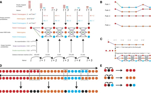
LB-Impute is a HMM-based method. Emission and transition probabilities are calculated from allelic depth of coverage and the physical distance between markers. The Viterbi algorithm (Rabiner 1989) is used to determine the most likely sequence of parental ancestry (hidden states) for each offspring in a biallelic population. Choosing the most likely sequence of hidden states, instead of the best state for each marker, re-duces the impact of individual erroneous markers in a data set. The assumption in the model is that markers are inde-pendent, in the sense that the emission and transition prob-abilities of a given marker will not influence the probprob-abilities of surrounding markers. Therefore, LB-Impute uses a first-order Markov chain.
trellis, (6) selection of the parental genotype at markert+ 1 in the highest-probability path as the next genotype in the final path, (7) regeneration of the Viterbi trellis from markers ttot + iusing the previous highest-probability path’s marker t + igenotype as the new marker M, (8) forward iteration of trellis markers across the entire chromosome, (9) reverse iteration of trellis windows across the entire chromosome, (10) comparison of the forward and reverse paths across the chromosome to determine a set of consensus genotypes for a given offspring, (11) setting of genotypes that conflict between paths to missing, (12) correcting of genotypes in the original data set that conflict with consensus calls to the con-sensus genotype, and (13) setting of missing genotypes be-tween concordant consensus calls in the original data set to the consensus genotypes. A more detailed explanation of key steps in the algorithm follows.
The initial step of the algorithm is to assign emission probabilities to each marker. Parental ancestry is the hidden state. Each read is assigned to a parent based on its sequence, and afinal emission probability is calculated based on the number of reads assigned to each parent and the probability of each read being erroneous. The emission probabilities for genetic contribution from a single parent, or homozygosity, at a given marker are calculated using the equation
EN ¼ ð1 2 errrÞRNðerrrÞR!N (1)
whereENis the emission probability of a given hidden state, or parental ancestry, N for the given genotype, errr is the probability of a sequencing error for each read at the position of a marker,RNis the number of reads with sequence match-ing the sequence of parentN, andR!Nis the number of reads with sequence not matching the genotype of parent N. The raw emission probability for the heterozygous hidden state is calculated using the equation
EH¼ 0:5RN
0:5R!N (2)
whereEHis the emission probability of the third hidden state, heterozygosity, or genetic contribution from both parents at a given site.
While the raw emission probability takes into account the likelihood that any one read is erroneous, genotyping errors independent of coverage also may affect a data set. These genotyping errors include misalignment of reads to the reference genome, resulting in the incorrect placement of a genotype, and an unannotated paralogous artifact. It is therefore desirable to limit both the minimum and maximum emission probabilities to minimize the chance of an artifact overinfluencing the final imputed genotypes. To do this, each emission probability at a given position is divided by the maximum emission probability at said position. Then each probability is divided by 1223errgandfinally has errgadded to it. The valueerrgrepresents the probability of a genotyping error. The maximum and minimum pos-sible emission probabilities for any given marker are
(1 2 errg)/(1 + errg) and errg/(1 + errg), respectively. Actual emission probabilities do not sum to 1 but instead will be constrained within these limits. The effect of emis-sion probabilities on the model is determined by their ra-tios rather than their sum.
In LB-Impute, the transition probabilities depend on the probability of recombination between markers. This bility depends on the distance between markers. The proba-bility of recombination is directly related to the distance in base pairs between markers. The equations used to calculate transition probabilities are
PS¼0:5
1þe2ðDistM=DistRÞ
(3)
and
PR¼0:5
12e2ðDistM=DistRÞ
(4)
where PS is the probability of maintaining a given hidden state, andPRis the probability of a recombination event caus-ing a change of hidden states. DistMis the distance in base pairs between two markers, and DistRis the distance in base pairs for transition probabilities to equalize. By default, we assume that two recombinations are required to transition from one homozygous parental state to the other homozy-gous parental state, resulting in double recombination events between proximal markers being heavily penalized com-pared to single events. In a population with many recombi-nation events (such as a recombinant inbred line), the user may choose to allow for double events to have the same transition probability as single recombination events.
The final modification to the standard Viterbi algorithm
(Rabiner 1989) is the use of a variable trellis window to identify recombination breakpoints. Because one of the as-sumptions in this program is that there may be a high rate of error for any one marker, the incorporation of information from multiple markers into a Markov chain may resolve this issue. While it would be ideal for this chain to stretch the entire length of the chromosome, it would be computation-ally inefficient to calculate the probability of every possible path through it, and therefore, an iterating-window approach is used. The user may select the number of markers to be incorporated into each trellis by changing the window size n. Within a window, the probabilities of every possible path between markertand markert+n(Figure 1A) are calcu-lated using the emission and transition probabilities de-scribed earlier. After the probabilities of every possible path for a given window are calculated, thet+ 1 hidden state of the path with the highest probability is selected (Figure 1B). Following this, the trellis is regenerated using the marker that wast+ 1 as the newt(Figure 1C).
on the chromosome. This generates two complete paths of hidden parental states across the entire chromosome. This approach is taken because, while the emission and transition probabilities will be the same for the forward and reverse paths, the value of the starting markertmay differ. Hidden-state calls that are concordant between the forward and re-verse paths are included in thefinal path. When the parental ancestry at a marker conflicts between the forward and re-verse paths, the corresponding marker is set to missing in the final path for said offspring (Figure 1D). This is done even if the marker has a call in the original data set because the algorithm has determined the call to be unreliable. If the user prefers to obtain as many imputed calls as possible, he or she may choose to use the state with the higher probability from the forward and reverse paths to determine a genotype for the marker. Missing markers are inferred by the state of the
flanking markers. When the states of theflanking marker are
concordant, the missing marker is resolved to the genotype of
theflanking markers. When they are discordant, the missing
marker is not imputed (Figure 1E).
In addition to being able to impute both missing and falsely homozygous genotypes in the offspring, the LB-Impute algo-rithm allows imputation of missing parental alleles. Dense
founder genotype maps are critical for interpreting markers and resolving recombination breakpoints with high resolution in many biallelic populations. Missing parental genotypes reduce the power of breakpoint resolution. To impute missing parental genotypes, parental haplotypes are recovered from observed markers in the offspring. The approach is similar to the one used to impute missing markers in the offspring. The difference is that the parental state of flanking markers is assigned to ambiguous rather than missing markers in each offspring. The consensus genotype, as determined across imputed offspring, for a missing parental marker is then assigned to the parent. Using this system of parental imputa-tion followed by offspring imputaimputa-tion as described by Huang et al.(2014), a high-resolution map can be generated from low-coverage sequencing data.
Algorithm testing
to one of the parents, producing a population in which only the recombination of the F1is observable, and homozygous alleles must come from the backcrossed parent. An F2 pop-ulation is the result of selfing an F1offspring to produce a biallelic population in which recombination can be observed on both chromosomes, and homozygous alleles from both parents are present. Performance comparisons were done with FSFHap.
Generation of simulated data:Simulated F1BC1and F2data sets were generated using a custom Java-implemented algo-rithm. The exact methodology for simulated data set con-struction is described in Supporting Information, File S1, Note 2. In total, 80 data sets, 40 F1BC1 and 40 F2, were generated, with coverage values spaced evenly from 1000 reads per sample (0.13coverage) up to 40,000 reads per sample (4.03 coverage). Twenty replicates were created for each data set.
The amount of missing or erroneous data was inversely proportional to read coverage. Missing datarefers to sites within a sample where there are no aligned reads, resulting in an absent genotype call. Erroneous data occur when in-complete allele recovery results in false homozygosity at a given site. For instance, the simulated F1BC143 coverage data sets had only 13.48% [60.34% (SD)] missing or erro-neous data, whereas the 0.13coverage data sets had a miss-ing or erroneous fraction of 95.16% [60.20% (SD)] (Figure S1A). For the 4.03 and 0.13F2data sets, the missing or erroneous fractions were 13.61% [60.48% (SD)] and 95.12% [60.34% (SD)], respectively (Figure S1B).
Preparation of real data: GBS data sets from a previously described B733Country Gentleman (B733CG) F2maize population (Heffelfingeret al.2014) and the IBM Maize RIL (Elshireet al.2011) data set were prepared as described in File S1, Note 3. For the B733CG data sets,five validation sets were generated with half the calls with seven aligned reads randomly removed. At a depth of seven reads, the chance of a false homozygote is only 1.56% (Swartset al. 2014). For the IBM Maize RIL population, five validation sets with half the markers with four aligned reads randomly removed were created. While it would have been preferable to use seven reads, the lower overall sequencing coverage resulted in most of the samples having zero markers with seven reads. While false homozygosity may have resulted in some of the markers being erroneous (12.5% of heterozy-gotes with four reads would be expected to be miscalled), the low levels of heterozygosity present in the data set ow-ing to repeated selfing would be expected to minimize this effect.
Algorithm settings
For the analyses described, FSFHap (Swarts et al. 2014), Beagle (Browning and Browning 2007), and Mendel Impute (Chiet al.2013) versions and settings are described inFile S1, Note 1. LB-Impute was set to its default parameters. For
emission probabilities, we assume a 5% resequencing error rate (errr) and a 5% genotype error rate (errg). To determine transition probabilities, a 10-Mbp recombination interval (DistR) was applied as described in Equations 3 and 4. We also used the default setting that transitions between homo-zygous parental states that are the product of two transition probabilities. The Markov trellis window was set to a length of 7. For the RIL data set, the double recombination events were treated as a single event.
Data availability
LB-Impute is publicly available at https://github.com/dellaporta-laboratory/LB-Impute. Test datafiles used in these analyses are also available on the Github site.
Results
Evaluation of LB-Impute was performed onfive distinct data set categories: two simulated F2and F1BC1populations, two maize B733CG F2populations, and one B733Mo17 RIL population. To evaluate the performance of LB-Impute, both the fraction of data imputed and the accuracy were mea-sured. Results from the LB-Impute analyses were compared with those of FSFHap (Bradbury et al. 2007; Swarts et al. 2014), a widely used program designed to deal with false homozygosity resulting from incomplete coverage of hetero-zygous markers. Like LB-Impute, FSFHap is designed specif-ically to impute biallelic populations. The performance of both programs was tested on the set of simulated data sets and real data sets. Additionally, Beagle and Mendel Impute, which are not designed to account for false homozygosity, were tested on simulated data sets.
LB-Impute and FSFHap performance on simulated data
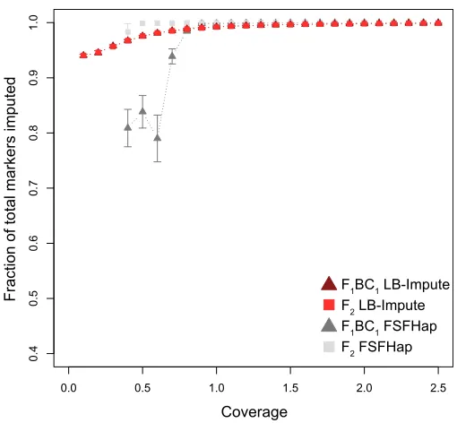
Thefirst parameter considered was the fraction of data that
was left missing in each imputed data set. LB-Impute left,1% of markers missing in the F1BC1and F2data sets at$0.93 coverage. The lowest fraction of markers imputed was 94.54% [60.36% (SD)]. FSFHap was unable to impute data sets in either the F1BC1or F2data sets at,0.43coverage but achieved.99% marker imputation in higher-coverage data sets (Figure S2).
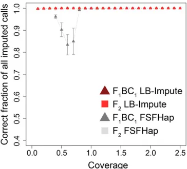
Both FSFHap and LB-Impute resolved all markers, not just those that were missing. Accordingly, absolute accuracy was measured as the fraction of nonmissing markers in thefinal imputed data sets that were correct (Figure 2). Importantly, LB-Impute achieved.99% accuracy in the F1BC1and F2data sets at all tested levels (0.1–2.53) of coverage. In contrast, for FSFHap, absolute accuracy$99% was achieved in most of the data sets, occurring with$0.83coverage in F1BC1and
Next, the fraction of recombination breakpoints imputed correctly (Figure S3A) and the mean number of missing markers around recombination breakpoints (Figure S3B) were evaluated. A recombination event was considered to be correctly imputed if the flanking imputed genotypes matched the true flanking genotypes of the recombination event. Missing markers were determined by the number of markers between the recombination event and the imputed genotypes. Again, LB-Impute was able to correctly impute recombination events with greater frequency in both the F2 (minimum accuracy 77.16%, maximum accuracy 90.09%) and F1BC1(minimum accuracy 76.87%, maximum accuracy 89.95%) populations than FSFHap (minimum accuracy 44.65%, maximum accuracy 80.71% for F2; minimum accu-racy 12.86%, maximum accuaccu-racy 63.07% for F1BC1). Most of the recombination events considered to be incorrectly im-puted were the result of the imim-puted breakpoint being slightly offset from the true event rather than erroneous gen-otyping. The greater accuracy of LB-Impute was somewhat at the expense of the absolute number of markers imputed. LB-Impute left more missing markers (minimum of 2.35 markers per event, maximum of 150.57 markers per event) than FSFHap (minimum 0.15, maximum 3.30) in both the F1BC1 and F2data sets.
Finally, it was observed that FSFHap greatly outperformed LB-Impute in terms of run time, with run times ranging from 3.95 to 46.95 sec. As discussed next, these run times increased, however, when LB-Impute was set for greatest accuracy by extending the length of the trellis window.
Effect of LB-Impute window length on performance
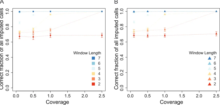
The length of the Markov trellis window in LB-Impute affects how much information is used to predict genotype, the trade-off being increased run times. To demonstrate this, window lengths of between 2 and 7 were tested on simulated F2 (Figure S4A) and F1BC1 (Figure S4B) 0.13, 0.53, 1.03, and 2.53coverage data sets. Both accuracy and run time were evaluated. At window length 2, accuracy fell between
66.69 and 70.70%. At window length 7, accuracy was.99% in all simulations, and at window length 6, accuracy was greater than.98% in all simulations. The accuracy of other simulations varied with window length and coverage in a similar fashion.
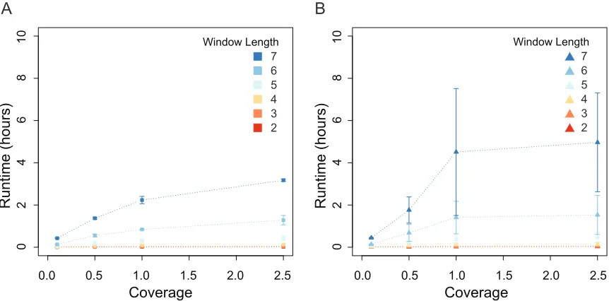
Window length also had an effect on the fraction of markers imputed. A window length of 2 resulted in only 39.38–43.01% of the markers being imputed in F2 populations, whereas longer window lengths saw greatly improved performance, with.94% of all markers being imputed by window length 7. Window size effect on run time was tested with a window size of 2, resulting in run times ranging from a minimum of 31.13 sec at 0.13coverage to a maximum of 17,878.90 sec at 2.53coverage with a window size of 7 (Figure S5, A and B).
Beagle and Mendel Impute performance
Beagle (Browning and Browning 2007) and Mendel Impute (Chiet al.2013) were tested on all simulated F2and F1BC1 data sets, and the results were compared to those of LB-Impute. In F1BC1data sets, Mendel Impute was able to impute at 98.76% [61.51% (SD)] accuracy at 2.53coverage and .90% accuracy at .1.53coverage. Below 1.53coverage, however, accuracy dropped off precipitously until reaching 50.10% [61.74% (SD)] at 1.13coverage. In F2data sets, it performed similarly at.1.53coverage and better below, with a minimum accuracy of 72.61% [61.50% (SD)] at 0.73 coverage (Figure S6A). Beagle had a maximum accuracy of 78.60% [61.00% (SD)] at 2.53coverage and a minimum of 50.69% [61.97% (SD)] in the F1BC1data sets. In the F2data sets, its maximum and minimum accuracies were 78.50% [60.73% (SD)] and 37.07% [60.19% (SD)] at 2.53 and 0.13coverage, respectively (Figure S6B).
LB-Impute and FSFHap performance on real data
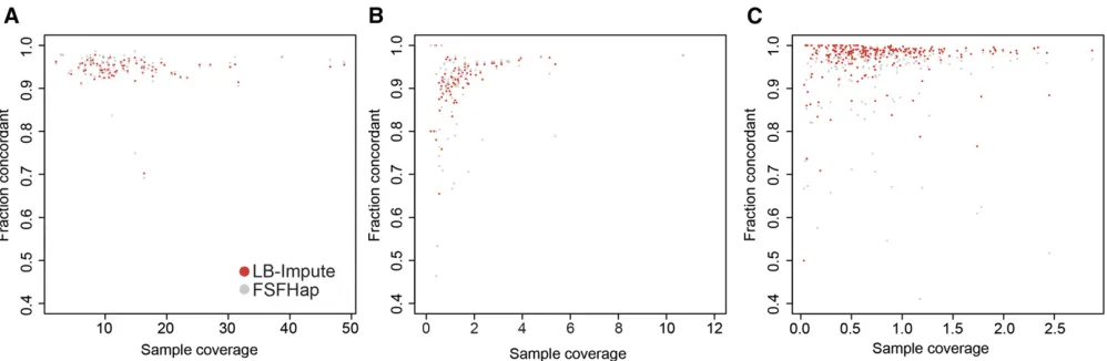
To determine the accuracy of LB-Impute on real sequencing data, it was tested on two GBS data sets generated from a maize B733CG F2population (Heffelfingeret al.2014) and the IBM Maize RIL population (Elshireet al.2011). One B73 3 CG data set, containing 11,219 postfilter markers, was generated from a HincII digest of both parents plus 89 off-spring (Figure 3A andFigure S7A). The other B733CG data set, produced byRsaI, had 127,144 postfilter markers iden-tified in both parents and 90 offspring (Figure 3B andFigure S7B). Finally, the IBM Maize RIL data set consisted of 14,493 postfilter markers typed in 275 offspring (Figure 3C and Fig-ure S7C). Of the 275 offspring, 255 had validation markers. The remaining 20 lacked sufficient sequencing coverage to contribute validation markers.
Using default parameters (trellis window size of 7), LB-Impute was able to impute a mean of 99.87% [60.01% (SD)] of all markers in HincII replicates and 99.18% [60.01% (SD)] inRsaI replicates. FSFHap imputed 98.27% [60.10% (SD)] of all markers in the HincII data set and 97.50% [60.45% (SD)] in theRsaI data set. In the IBM Maize RIL data set, LB-Impute and FSFHap were able to impute 93.92% [60.01% (SD)] and 99.15% [60.01% (SD)] of the markers, respectively.
Concordance between imputed genotypes and the valida-tion set was 94.62% [63.02% (SD)] inHincII data sets and 91.44% [66.73% (SD)] inRsaI data sets. For FSFHap, mean concordance was 94.71% [64.05% (SD)] forHincII data sets and 89.70% [69.76% (SD)] forRsaI data sets. In the IBM Maize RIL population, LB-Impute concordance was 96.98% [65.14% (SD)], and FSFHap concordance was 93.27% [611.24% (SD)]. LB-Impute performed significantly better than FSFHap for the RsaI (P= 0.045) and IBM Maize RIL data sets (P , 0.001), as evaluated by paired two-tailed t-test. LB-Impute and FSFHap produced comparable results for theHincII population (P= 0.70). LB-Impute mean run time was 5323.66 sec [68.79 sec (SD)] forHincII repli-cates, 50,248.17 sec [6402.60 sec (SD)] for RsaI repli-cates, and 7092.82 sec [6380.97 sec (SD)] for the IBM Maize RIL data set. These run times are for the entire data set rather than each individual. Run times for FSFHap were not taken because multiple manual steps were required during the imputation process. As with the simulated data, the FSFHap algorithm itself was considerably faster than LB-Impute.
Discussion
Imputation algorithms have been critical for enhancing gen-otyping studies. While originally used to resolve calls missing in merged data sets and to increase the power of genome-wide association studies, new demands have been placed on this field of bioinformatics. One such demand has emerged from low-coverage genome resequencing of plant populations. LB-Impute resolves missing and erroneous data in these popula-tions by incorporating allelic depth of coverage and physical distance between markers into a HMM.
Simulated data indicated that LB-Impute is highly suited for resolving missing and erroneous data, even at extremely low levels of coverage. Accuracy.99% was achieved at all tested levels of coverage ($0.13) in both F2and F1BC1data sets. LB-Impute performed especially well compared to meth-ods not designed for dealing with the issues associated with
low-coverage sequencing (e.g., false homozygosity), such as Beagle (Browning and Browning 2007) and Mendel Impute (Chiet al.2013). At 0.13coverage, LB-Impute was able to maintain accuracy .99%, while both Beagle and Mendel Impute fell to as low as 37.07 and 49.51%, respectively. LB-Impute’s performance, however, was highly dependent on window size. With a window length of 6 or 7, the tradeoff for high accuracy was a dramatic increase in run time.
LB-Impute was tested on two maize GBS data sets (Heffelfinger et al.2014) and the IBM Maize RIL population (Elshireet al. 2011) In the B733CG data sets, LB-Impute performed similarly to FSFHap with theHincII data set but slightly better with the RsaI and RIL data sets. Finally, it is worth noting that the true accuracy of the imputation results may be higher than the con-cordance because results corrected by imputation are likely to be more reliable than unimputed genotypes (Swartset al.2014).
A limitation to LB-Impute is that it is not designed to handle data from populations with more than two alleles. As the number of segregating haplotypes within the population increases, the number of hidden states expands according to the equation
nðn21Þ
2 þn (5)
wherenis the number of parental haplotypes. Given how the Viterbi trellis window is constructed, this results in an exponen-tial increase in the number of possible paths through hidden states that must be solved. Going from a biallelic to a triallelic population results in an increase in the number of paths by a factor of 2(o+ 1), whereois equal to the trellis window of the Viterbi algorithm. Compounding this problem is that as the number of parental haplotypes increases, the informative con-tent of each individual marker decreases. To distinguish be-tween haplotypes, the number of biallelic markers must be
n#2m (6)
biallelic markers are required to distinguish between five haplotypes, and so on. Therefore, the trellis window de-scribed in this algorithm must increase with the number of segregating haplotypes to maintain the same level of power. Ultimately, the increase in computing time would cripple per-formance for even relatively simple multiallelic populations such as multiparent advanced generation intercross (MAGIC) lines (Cavanaghet al.2008). One approach to resolving this issue with LB-Impute would be to eliminate the ability to compute the heterozygous state for highly homozygous pop-ulations. Homozygous populations, such as RILs, may contain residual heterozygosity owing to incomplete fixation of al-leles or unintended outcrossing. The ability to identify lines with heterozygosity in populations that have undergone re-peated selfing is a desirable objective.
As compared to FSFHap, LB-Impute should be used for imputing populations when parental genotypes are available. FSFHap’s ability to recover parental haplotypes without di-rect parental genotyping makes it useful for imputing large populations with no parental sequencing. Outside of these cases, such as large populations with parental sequencing, our results indicate the LB-Impute and FSFHap would per-form similarly.
Conclusions
A critical goal in population genomics is to develop impu-tation methods suitable to detect heterozygosity and re-combination in low-coverage data sets. We have successfully implemented a solution to this problem that allows for ac-curate parental and offspring imputation in low-coverage sequencing data sets in biallelic populations. The resulting algorithm, LB-Impute, is able to reliably resolve both missing data and false homozygosity even for samples with less than 13coverage.
Challenges remain, however, especially in multiparen-tal populations with more than two segregating alleles. Many populations used for agricultural breeding and re-search meet this description. Without reliable methods for resolving missing and erroneous data, the power of low-coverage multiplexed sequencing in these populations will be limited. While the method described in this paper is not suitable for populations with more than two alleles, it does identify read coverage as a key parameter for resolving this challenge.
The next generation of imputation algorithms for low-coverage sequencing data will benefit from using read cover-age when identifying alleles present in a sample. By adjusting the probability of observed genotypes based on coverage com-bined with information about haplotype frequency gleaned from identical-by-descent (IBD) regions across samples, het-erozygous regions will be more likely to be accurately phased. The need for considerable IBD homozygosity or phased pa-rental haplotypes is unlikely to go away with improved algo-rithms and will instead most likely be remedied by long-read sequencing on all or part of a population.
Acknowledgments
We thank Yingchun Tong and Maria Moreno for preparing the B733CG genome libraries. Sequencing was performed at the Yale Center for Genome Analysis. We also thank Mathias Lorieux for his comments on the development of LB-Impute. This work was supported by grants to S.L.D. from the National Science Foundation (NSF) (0965420 and 1419501), the National Institutes of Health (NIH), and the Bill and Melinda Gates Foundation. C.A.F. was sup-ported by a NIH Biomedical Informatics Research Training grant. C.H. was supported by the NSF and the Bill and Melinda Gates Foundation. H.Z. was supported by NIH grant R01-GM59507. Computational analyses were per-formed on the Yale University Biomedical High Performance Computing Cluster, which is supported by NIH grants RR-19895 and RR-029676-01.
Author contributions: C.A.F. assisted in developing the concept of the algorithm, wrote several prototype versions of LB-Impute, performed comparison tests using FSFHap, and drafted the manuscript. C.H. assisted in developing the concept for the algorithm, wrote the final LB-Impute algorithm, developed the simulated data sets, prepared the real data sets, performed testing on simulated data sets, and drafted the manuscript. H.Z. and S.L.D. provided conceptual support for development of the algorithm and analyses and assisted in drafting the manuscript. The authors declare that they have no competing interests.
Literature Cited
Bamshad, M. J., S. B. Ng, A. W. Bigham, H. K. Tabor, M. J. Emond
et al., 2011 Exome sequencing as a tool for Mendelian disease gene discovery. Nat. Rev. Genet. 12: 745–755.
Bradbury, P. J., Z. Zhang, D. E. Kroon, T. M. Casstevens, Y. Ramdoss
et al., 2007 TASSEL: software for association mapping of com-plex traits in diverse samples. Bioinformatics 23: 2633–2635. Broman, K. W., and S. Sen, 2009 A Guide to QTL Mapping with R/
qtl. Springer, New York.
Broman, K. W., H. Wu, ´S. Sen, and G. A. Churchill, 2003 R/qtl: QTL mapping in experimental crosses. Bioinformatics 19: 889– 890.
Browning, B. L., and S. R. Browning, 2009 A unified approach to genotype imputation and haplotype-phase inference for large data sets of trios and unrelated individuals. Am. J. Hum. Genet. 84: 210–223.
Browning, S. R., and B. L. Browning, 2007 Rapid and accurate haplotype phasing and missing-data inference for whole-genome association studies by use of localized haplotype clustering. Am. J. Hum. Genet. 81: 1084–1097.
Browning, S. R., and B. L. Browning, 2011 Haplotype phasing: existing methods and new developments. Nat. Rev. Genet. 12: 703–714.
Cavanagh, C., M. Morell, I. Mackay, and W. Powell, 2008 From mutations to MAGIC: resources for gene discovery, valida-tion and delivery in crop plants. Curr. Opin. Plant Biol. 11: 215–221.
Cleveland, M. A., J. M. Hickey, and B. P. Kinghorn, 2011 Genotype imputation for the prediction of genomic breeding values in non-genotyped and low-density genotyped individuals. BMC Proc. 5(Suppl. 3): S6.
Elshire, R. J., J. C. Glaubitz, Q. Sun, J. A. Poland, K. Kawamoto
et al., 2011 A robust, simple genotyping-by-sequencing (GBS) approach for high diversity species. PLoS One 6: e19379. Fuchsberger, C., G. R. Abecasis, and D. A. Hinds, 2015 minimac2:
faster genotype imputation. Bioinformatics 31: 782–784. Hawley, M. E., and K. K. Kidd, 1995 HAPLO: a program using the
EM algorithm to estimate the frequencies of multi-site haplo-types. J. Hered. 86: 409–411.
Heffelfinger, C., A. C. Fragoso, M. A. Moreno, J. D. Overton, J. P. Mottinger et al., 2014 Flexible and scalable genotyping-by-sequencing strategies for population genomics. BMC Genomics 15: 979.
Howie, B. N., P. Donnelly, and J. Marchini, 2009 Aflexible and accurate genotype imputation method for the next generation of genome-wide association studies. PLoS Genet. 5: e1000529. Huang, B. E., C. Raghavan, R. Mauleon, K. W. Broman, and H.
Leung, 2014 Efficient imputation of missing markers in low-coverage genotyping-by-sequencing data from multiparental crosses. Genetics 197: 401–404.
International HapMap Consortiumet al., 2010 Integrating com-mon and rare genetic variation in diverse human populations. Nature 467: 52–58.
Li, Y., C. J. Willer, J. Ding, P. Scheet, and G. R. Abecasis, 2010 MaCH: using sequence and genotype data to estimate haplotypes and unobserved genotypes. Genet. Epidemiol. 34: 816–834.
Li, Y., C. Sidore, H. M. Kang, M. Boehnke, and G. R. Abecasis, 2011 Low-coverage sequencing: implications for design of complex trait association studies. Genome Res. 21: 940–951. Liu, E. Y., M. Li, W. Wang, and Y. Li, 2013 MaCH‐Admix:
geno-type imputation for admixed populations. Genet. Epidemiol. 37: 25–37.
Long, J. C., R. C. Williams, and M. Urbanek, 1995 An EM algo-rithm and testing strategy for multiple-locus haplotypes. Am. J. Hum. Genet. 56: 799.
Marchini, J., B. Howie, S. Myers, G. McVean, and P. Donnelly, 2007 A new multipoint method for genome-wide association studies by imputation of genotypes. Nat. Genet. 39: 906–913. Miller, M. R., J. P. Dunham, A. Amores, W. A. Cresko, and E. A.
Johnson, 2007 Rapid and cost-effective polymorphism identi-fication and genotyping using restriction site associated DNA (RAD) markers. Genome Res. 17: 240–248.
Nielsen, R., J. S. Paul, A. Albrechtsen, and Y. S. Song, 2011 Genotype and SNP calling from next-generation se-quencing data. Nat. Rev. Genet. 12: 443–451.
Niu, T., Z. S. Qin, X. Xu, and J. S. Liu, 2002 Bayesian haplotype inference for multiple linked single-nucleotide polymorphisms. Am. J. Hum. Genet. 70: 157–169.
1000 Genomes Project Consortiumet al., 2012 An integrated map of genetic variation from 1,092 human genomes. Nature 491: 56–65.
Qin, Z. S., T. Niu, and J. S. Liu, 2002 Partition-ligation-expectation-maximization algorithm for haplotype inference with single-nucleotide polymorphisms. Am. J. Hum. Genet. 71: 1242– 1247.
Rabiner, L., 1989 A tutorial on hidden Markov models and se-lected applications in speech recognition. Proc. IEEE 77: 257– 286.
Rowan, B. A., V. Patel, D. Weigel, and K. Schneeberger, 2015 Rapid and inexpensive whole-genome genotyping-by-sequencing for crossover localization and fine-scale genetic mapping. G3 5: 385–398.
Scheet, P., and M. Stephens, 2006 A fast and flexible statistical model for large-scale population genotype data: applications to inferring missing genotypes and haplotypic phase. Am. J. Hum. Genet. 78: 629–644.
Spencer, C. C., Z. Su, P. Donnelly, and J. Marchini, 2009 Designing genome-wide association studies: sample size, power, imputation, and the choice of genotyping chip. PLoS Genet. 5: e1000477.
Stephens, M., and P. Donnelly, 2003 A comparison of bayesian methods for haplotype reconstruction from population genotype data. Am. J. Hum. Genet. 73: 1162–1169.
Stephens, M., N. J. Smith, and P. Donnelly, 2001 A new statistical method for haplotype reconstruction from population data. Am. J. Hum. Genet. 68: 978–989.
Swarts, K., H. Li, J. A. Romero Navarro, D. An, M. C. Romayet al., 2014 Novel methods to optimize genotypic imputation for low-coverage, next-generation sequence data in crop plants. Plant Genome 7: 1–12.
Wu, X., C. Ren, T. Joshi, T. Vuong, D. Xuet al., 2010 SNP discov-ery by high-throughput sequencing in soybean. BMC Genomics 11: 469.
Yu, J., J. B. Holland, M. D. McMullen, and E. S. Buckler, 2008 Genetic design and statistical power of nested associa-tion mapping in maize. Genetics 178: 539–551.
GENETICS
Supporting Information www.genetics.org/lookup/suppl/doi:10.1534/genetics.115.182071/-/DC1
Imputing Genotypes in Biallelic Populations from
Low-Coverage Sequence Data
Christopher A. Fragoso, Christopher Heffelfinger, Hongyu Zhao, and Stephen L. Dellaporta
File S1
Supplemental materials and methods
Supplemental Note
A
: Imputation algorithm parameters
FSFHap version 5.2.6 was used for imputation. For simulated datasets, the only
non-default setting was Window LD as true. For the real B73xCG F
2datasets (Heffelfinger et
al. 2014), minhap was 2 to impute over the low coverage real data. For the IBM Maize
RIL population (Elshire et al. 2011), Window LD was true and minhap was set to 2. The
BC option was set as false. Tassel graphical user interface version of FSFHap was used
for the real B73xCG F
2data and the IBM Maize RIL data (Bradbury et al. 2007).
Correspondence with the authors of FSFHap provided guidance as to properly calibrate
FSFHap for low coverage data.
Beagle (Browning and Browning 2007) version 4.1 was used for imputation of simulated
F
1BC
1and F
2datasets. Default settings were used. The matrix completion method,
Mendel Impute v 2012 (Chi et al. 2013) used the highest-performing window setting as
described by the authors of the method (window size = 75).
Supplemental Note
B
: Generation of simulated data
Generation of simulated F
1BC
1and F
2datasets was performed using custom Java scripts
as follows. Sequencing reads were not simulated; instead, two final genotype datasets
were directly generated for each set of conditions. The first, an “actual” dataset, consists
of a VCF file with true genotypes for each sample. The second, a “coverage-modified”
dataset, involved first randomly distributing a finite number of “reads” between markers
based on a binomial model. Then, final genotypes are determined by distributing these
reads between possible alleles, also based on a binomial model.
To explain further, “actual” and “coverage-modified” genotypes for a total of 200
offspring in each dataset were determined on a 100 Mbp chromosome with 10,000
polymorphic sites. Each sample was assigned a mean of three recombination events (± 2
(SD)) that were placed at random locations on the chromosomes. It is worth noting that
each individual chromosome was not simulated, rather, recombination breakpoints were
placed randomly across the dataset and then marker genotypes determined as described as
below. Therefore, the same distribution of recombination event counts was expected for
both the simulated F
1BC
1and F
2populations.
between alleles at each marker using a binomial model as described above in the
"Coverage Modified" dataset. When only one of the two alleles at a heterozygous marker
received sequencing coverage, that marker was changed into a homozygote depending on
which marker had sequencing coverage. Parental calls were always accurate in these
datasets.
Supplemental Note
C
: Generation of real data
To prepare real data for testing with LB-Impute and FSFHap, GBS sequencing data from
a previously described B73xCG F
2population (Heffelfinger et al. 2014) and the IBM
Maize RIL population (Elshire et al. 2011) were used. Reads from these datasets were
first aligned to the B73 reference genome (Zea mays refgen v2) via NovoAlign
0
500000
1000000
1500000
2000000
0 0.5 1 1.5 2 2.5 3 3.5 4
Marker count
Mean dataset coverage
0
500000
1000000
1500000
2000000
0 0.5 1 1.5 2 2.5 3 3.5 4
Mean dataset coverage
Marker count
Missing markers Erroneous markers
A B
Figure S1 Counts of missing and erroneous markers in each simulated A) F1BC1 and B) F2
dataset.
0.0 0.5 1.0 1.5 2.0 2.5
0.4
0.5
0.6
0.7
0.8
0.9
1.0
F1BC1 LB-Impute
F2 LB-Impute
F1BC1 FSFHap
F2 FSFHap
Fraction of total markers imputed
Coverage
Figure S2 Fraction of total markers called by LB-Impute and FSFHap.Called markers refer to
0.0 0.5 1.0 1.5 2.0 2.5
0.0
0.2
0.4
0.6
0.8
1.0
0.0 0.5 1.0 1.5 2.0 2.5
100
150
200
50
0
Mean missing markers per recombination event
A
B
F1BC1 LB-Impute F2 LB-Impute F1BC1 FSFHap F2 FSFHap
Fraction of recombination events identified correctly
Coverage
Coverage
Figure S3 Recombination event identification A) accuracy and B) mean missing marker count for
LB-Impute and FSFHap.
0.0 0.5 1.0 1.5 2.0 2.5
0.0
0.2
0.4
0.6
0.8
1.0
Correct fraction of all imputed calls
Coverage
Window Length
0.0 0.5 1.0 1.5 2.0 2.5
0.0
0.2
0.4
0.6
0.8
1.0
Correct fraction of all imputed calls
Coverage
A
B
7 6 5 4 3 2
Window Length
7 6 5 4 3 2
Figure S4 Effect of LB-Impute window length on imputation accuracy for A) F2 and B) F1BC1
0.0 0.5 1.0 1.5 2.0 2.5
Coverage
0
2
4
6
8
10
Runtime (hours)
A
0.0 0.5 1.0 1.5 2.0 2.5
Coverage
0
2
4
6
8
10
Runtime (hours)
B
Window Length 7 6 5 4 3 2 Window Length
7 6 5 4 3 2
Figure S5 Effect of LB-Impute window length on runtime for A) F2 and B) F1BC1 simulated data.
0.0 0.5 1.0 1.5 2.0 2.5
0.3
0.4
0.5
0.6
0.7
0.8
0.9
1.0
0.0 0.5 1.0 1.5 2.0 2.5
0.3
0.4
0.5
0.6
0.7
0.8
0.9
1.0
Coverage Coverage
Correct fraction of all imputed calls
Correct fraction of all imputed calls
A
B
F1BC1 LB-Impute F2 LB-Impute F1BC1 Beagle F2 Beagle F1BC1 LB-Impute
F2 LB-Impute F1BC1 Mendel Impute F2 Mendel Impute
Figure S6 Accuracy of A) Mendel Impute and B) Beagle imputation on simulated datasets
compared to LB-Impute.
Sample coverage
A B
Sample coverage
10 12
Standard deviation sample concordance
0 2 4 6 8
Standard deviation sample concordance
LB-Impute FSFHap
10 20 30 40 50
0.00
0.05
0.10
0.15
0.20
0.00
0.05
0.10
0.15
0.20
0.0 0.5 1.0 1.5 2.0 2.5
0.00
0.05
0.10
0.15
0.20
Sample coverage
Standard deviation sample concordance
Figure S7 Sample coverage versus standard deviation of concordance for A) RsaI B73xCG data, B) HincII B73xCG data, and C) IBM Maize RIL data. The standard deviation of concordance between the imputed and validation sets (five replicates) was calculated for each sample in the HincII and RsaI B73xCG F2 datasets. Mean concordance is given in Figure 3.