Local properties of patterned vegetation: Quantifying endogenous and exogenous effects

, 20120359, published 4 November 2013

371

2013

Phil. Trans. R. Soc. A

Gopal G. Penny, Karen E. Daniels and Sally E. Thompson

quantifying endogenous and exogenous effects

Local properties of patterned vegetation:

Supplementary data

rsta.2012.0359.DC1.html

http://rsta.royalsocietypublishing.org/content/suppl/2013/10/28/

"Data Supplement"

References

59.full.html#ref-list-1

http://rsta.royalsocietypublishing.org/content/371/2004/201203

Subject collections

(37 articles)

hydrology

collections

Articles on similar topics can be found in the following

Email alerting service

http://rsta.royalsocietypublishing.org/subscriptions

go to:

Phil. Trans. R. Soc. A

To subscribe to

on November 4, 2013

rsta.royalsocietypublishing.org

rsta.royalsocietypublishing.org

Research

Cite this article:Penny GG, Daniels KE, Thompson SE. 2013 Local properties of patterned vegetation: quantifying

endogenous and exogenous effects. Phil Trans R Soc A 371: 20120359.

http://dx.doi.org/10.1098/rsta.2012.0359

One contribution of 13 to a Theme Issue ‘Pattern formation in the geosciences’.

Subject Areas: hydrology

Keywords:

arid ecosystems, pattern formation, Fourier analysis

Author for correspondence: Gopal G. Penny

e-mail: [email protected]

Electronic supplementary material is available at http://dx.doi.org/10.1098/rsta.2012.0359 or via http://rsta.royalsocietypublishing.org.

Local properties of patterned

vegetation: quantifying

endogenous and

exogenous effects

Gopal G. Penny

1

, Karen E. Daniels

2

and

Sally E. Thompson

1

1

_{Department of Civil and Environmental Engineering,}

University of California, Berkeley, CA 94710, USA

2

_{Department of Physics, North Carolina State University, Raleigh,}

NC 27695, USA

Dryland ecosystems commonly exhibit periodic bands of vegetation, thought to form due to competition between individual plants for heterogeneously distributed water. In this paper, we develop a Fourier method for locally identifying the pattern wavenumber and orientation, and apply it to aerial images from a region of vegetation patterning near Fort Stockton, TX, USA. We find that the local pattern wavelength and orientation are typically coherent, but exhibit both rapid and gradual variation driven by changes in hillslope gradient and orientation, the potential for water accumulation, or soil type. Endogenous pattern dynamics, when simulated for spatially homogeneous topographic and vegetation conditions, predict pattern properties that are much less variable than the orientation and wavelength observed in natural systems. Our local pattern analysis, combined with ancillary datasets describing soil and topographic variation, highlights a largely unexplored correlation between soil depth, pattern coherence, vegetation cover and pattern wavelength. It also, surprisingly, suggests that downslope accumulation of water may play a role in changing vegetation pattern properties.

1. Introduction

Pattern formation occurs in numerous ecological and biological systems, where it has been linked to reaction– diffusion (Turing)-type instabilities [1], hydrodynamic

2

rsta.r

oy

alsociet

ypublishing

.or

g

Phil

Tra

ns

R

Soc

A

37

1:

2012035

9

...

instabilities [2] and potential (variational) dynamics that maximize or at least increase ecological productivity [3,4]. Patterns have been observed in dryland vegetation [5], in bogs and wetlands [6,7], in mussel beds [8], termite mounds [4] and other systems [9]. In many cases, ecological patterns form an intermediate realization between environmental states in which the entire landscape is either colonized or bare. As such they often indicate the presence of bistable states, which are characterized by the potential for critical and locally irreversible transitions [10]. Both observations and theoretical work suggest that transitions between vegetated and desertified (unvegetated) conditions in patterned systems are preceded by striking changes in the morphology of the vegetation patterns, which thus act as an early-warning sign of deteriorating ecosystem health [11]. Understanding the controls on the morphology of vegetation patterns therefore has practical interest in terms of ensuring that observed changes are interpreted correctly.

Vegetation pattern formation in dryland ecosystems is a global phenomenon, ranging from random distributions of bare soil and vegetation canopies [12] to highly organized spatial distributions with identifiable length scales and orientations [1,5,13]. Intermediate cases such as power-law (scale-free) clustering [14–16], and dendritic structures in which vegetation concentrates along drainage lines [17,18] are also observed. All of these morphologies can be related to the presence, strength and directionality of positive feedbacks that concentrate resources (such as nutrients, soil carbon and water) that sustain plant life in a localized region near the plants [19–24]. These feedbacks have led to the moniker ‘ecosystem engineers’ being applied to perennial plants in dryland ecosystems: they create the conditions necessary for their own survival [25,26].

The formation of periodic vegetation patterns is strongly linked to the coupling of (i) water redistribution to the vicinity of plants and (ii) competition between individual plants for access to this water resource [3,5,27,28]. The dynamics of patterned vegetation systems has formed a focus of ecohydrological and nonlinear dynamics research, motivated by the increasingly well-demonstrated connection between pattern morphology and desertification risk [1,11,29,30]; and by the inherently interesting nonlinear dynamics of these systems [3,31]. Field and theoretical work has identified the important roles of vegetation dynamics [11], seed dispersal processes [32,33], root morphology [3,29], surface flow dynamics [34] and climate feedbacks [35] in modulating pattern morphology.

While our understanding of vegetation pattern dynamics is improving, there remain undeniable differences between simulated vegetation patterns and the natural ones observed in the field. Natural patterns are characterized by a degree of disorder and heterogeneity on multiple scales that is not reproduced in idealized models. Disorder can arise intrinsically through the existence of a range of stable wavelengths and orientations, with transitions in space and time occurring through local pattern defects [36]. In addition, the pattern wavelength and orientation can be strongly influenced by either wavelength-scale inhomogeneities [37] or larger gradients [38] in the underlying system, as well as the presence of boundaries [39] or noise [40].

3

rsta.r

oy

alsociet

ypublishing

.or

g

Phil

Tra

ns

R

Soc

A

37

1:

2012035

9

...

periodic boundary conditions, vegetation bands formed with a single wavelength and were orientated at 90◦ to the direction of water flow, in agreement with other modelling studies. When realistic boundary conditions were imposed, however, the bands near the top of the hillslope curved to lie perpendicular to the ridgeline. Similarly, the effects of spatial heterogeneity in soil properties on pattern formation have not been widely explored (although see [32]). A number of theoretical studies indicate that local biomass, band properties and band coherence should vary with changing minimum and maximum infiltration capacities and soil properties [41,42], and there are some tantalizing hints that subsurface features, such as the ironstone underlying tiger bush in Niger, calcrete hardpans underlying banded patterns in Texas, and silcrete hardpans underlying mulga bands in Australia [43–45], may have an association with patterned vegetation.

Predictions about the interaction of vegetation patterns with changing soil or topography can be investigated using remotely sensed datasets, an approach with a long and growing history. Vegetation patterns in Africa were first observed from light aircraft flights [46,47]. Initial analyses of the patterns demonstrated their spatial regularity on the basis of the two-dimensional Fourier power spectrum [48]. More recently, Deblauweet al.[30] undertook large-scale analyses of morphological trends in vegetation patterns in the Sudan by linking several remotely sensed datasets: surface imagery from the System for Earth Observation (SPOT) satellite, topographic data from the Shuttle Radar Topography Mission (STRM), and rainfall data from the Tropical Rainfall Measuring Mission (TRMM). This allowed analysis of pattern morphology at 400 m resolution over multiple square kilometres. Although higher resolution datasets are available, they have generally either been analysed only over relatively small spatial scales (≈1 km2) [29] or investigated from the perspective of identifying morphological change over time [49].

A key open question is therefore to characterize small-scale irregularities in vegetation patterns, and to classify them based on whether they arise due to either endogenous dynamics or variation in exogenous features imposed by the landscape. Understanding the implications of such variation on the resilience and stability of ecosystems has important consequences for identifying and preventing potential desertification.

In this paper, we report on the development of methods suitable for quantifying local patterns within high-resolution aerial photography, and for relating those features to ancillary datasets describing soil and topographic variation. Our site, located near Fort Stockton, TX, USA [43], was selected because it exhibits vegetation bands and also offers several characteristics that facilitate studies of covariation. First, the aerial photography covers a large region at a resolution (0.5 and 1 m) comparable to the diameter of perennial vegetation canopies, allowing for the observation of individual plants. Second, high-resolution (10 m spatial, 15 cm vertical) elevation datasets are available from the US National Elevation Dataset (NED), allowing changes in the orientation and gradient of the hillslope to be mapped on scales that are much smaller than the pattern wavelength. Finally, the study area has been mapped as part of the Soil Survey Geographic (SSURGO) national soils database, and contains considerable variation in soil type. The availability of these datasets provides a valuable opportunity to investigate correlations between vegetation patterning and soil characteristics over tens of square kilometres.

4

rsta.r

oy

alsociet

ypublishing

.or

g

Phil

Tra

ns

R

Soc

A

37

1:

2012035

9

...

null hypothesis: (3) large-scale variations in pattern properties can be explained by the nonlinear interactions associated with vegetation pattern formation.

We test the major hypotheses through the development of a localized Fourier technique to identify pattern wavenumber and direction. To address Hypothesis 1, this technique was applied to high (0.5 m) resolution aerial photography. To address Hypothesis 2, the technique was applied to a 188 km2_{area, allowing local pattern properties to be correlated with the site soil and} topographic properties. Hypothesis 3 was tested by identifying a subset of the 0.5 m resolution image containing banded patterns that were close to ideal (i.e. reproducible by a model). We applied the Fourier analysis technique to both observed and simulated patterns, and compared variability in the wavenumber and direction fields in the modelled and observed patterns.

We find that our two major hypotheses are satisfied. Local patterns are oriented in the same direction as the topographic slope and the pattern wavelength decreases for steeper gradients. Deviations from these trends are associated with the presence of ridges, stream channels, anthropogenic features or changes in soil type. Different soil types within the study area determine the pattern boundaries and the pattern morphology: shallow soils are associated with highly coherent, shorter wavelength patterns, and deep soils with patterns that become incoherent and increase in wavelength near stream channels. Finally, the modelling test validated our decision to focus on landscape and soil features. Even in the most uniform region of the observed patterns, the variability in the real pattern properties exceeded that which could be retained in the steady-state solution of a physical model that closely reproduced the mean pattern properties.

2. Material and methods

(a) Study site and data

The study site is a 188 km2area located approximately 30 km northwest of Fort Stockton, TX, USA (coordinates: 31◦05N, 103◦03W) [51]. The climate is hot and dry, with 370 mm annual rainfall on average, mean summer maximum temperatures of approximately 35◦C and winter minima near freezing. The site is part of a large cattle ranch and is used for grazing. Dominant vegetation species include tarbush (Flourensia cenua), bunch and sod grasses (Aristida purpurea, Bouteloua curtipendulaandScleropogon brevifolius), and mixed mesquite (Prosopsis glandulosa) and juniper (Juniperus pinchotti) brush [43]. The site contains a striking spatial pattern consisting of bands of continuous vegetation cover lying over bare soil [43] (figure 1).

High-resolution imagery (0.5 and 1 m pixels) were obtained from Digital Globe, and from the National Agricultural Imaging Project (NAIP) [52]. We used the highest resolution images from Digital Globe for fine-scale analysis and a comparison between modelled and observed pattern morphology. We analysed the NAIP images, which cover the whole area, to relate local pattern properties to soil and topographical features.

We classified the image pixels as ‘vegetation’ or ‘no vegetation’ using a supervised classification based on total brightness [53]. We used brightness because the perennial vegetation was not actively photosynthesizing when the photographs were taken, meaning that standard vegetation indices could not discriminate the vegetated locations. An example of the resulting binary image is shown in figure 1. Darker colours represent vegetation cover and the lighter colours bare soil. The insets show an original and classified image over a 260×260 m2window. We obtained elevation data from the NED provided by the US Geological Survey and soil maps from the SSURGO Database.

(b) Fourier windowing method

5

rsta.r

oy

alsociet

ypublishing

.or

g

Phil

Tra

ns

R

Soc

A

37

1:

2012035

9

...

(a)

(b)

(c)

Figure 1.(a) Binary image of the Fort Stockton region, covering an area of approximately 188 km2. Vegetation is shown as black and bare soil is shown in white. (b) Detail of size 260×260 m2, showing the original detailed image. (c) Binary image detail. (Online version in colour.)

short-time Fourier transforms or wavelet-based approaches used in timeseries analysis [54, 55]. Local wavevectors are useful for classifying convection patterns [56] and for identifying pattern defects [57,58]. Here, we applied a two-dimensional Fourier transform to obtain the power spectrum within a square, moving window. Local wavelength and pattern orientation were identified for each window, and the results averaged for all windows that spanned a given location. This straightforward technique is suitable for identifying the dominant pattern properties in noisy images with irregular patterning. More elegant and rigorously local techniques, based on the ratios of the spatial derivative of the banding pattern [57], could not be applied because the vegetation bands deviate substantially from a sinusoidal pattern in space. The drawbacks of the short-time Fourier transform—namely the tendency to truncate long wavelengths due to the finite window size, and poor localization of short-wavelength components [59]—do not pose significant difficulties in the current application, provided that the window is appropriately sized with respect to the local wavelength of the pattern.

For each window of size L×L, we obtained the two-dimensional fast Fourier transform

˜

f(kx,ky) of the patternf(x,y). For each window’sf˜(k), we calculated the power spectrumS(k)=

|˜f(k)|2_{. AsLincreases, the likelihood of identifying a single wavelength and orientation decreases.} Conversely, as Ldecreases, thek-resolution in Fourier space is reduced. To optimize both the localization of measurements and the resolution, we choseLto be at least 5λ. The window was applied to overlapping regions of the pattern at 20 m intervals.

The power spectrum measures the power contributed to the pattern by each wavevectork. To separate the local wavelength from its orientation, we decomposed eachk into its magnitude (wavenumber) k=

6

rsta.r

oy

alsociet

ypublishing

.or

g

Phil

Tra

ns

R

Soc

A

37

1:

2012035

9

...

binnedS(k) into annular rings of widthk=6π/L. To deconvolve the natural 1/kscaling of the image [60,61], we computed the total power within each annular ring,S(k). The location peak of this total power (rather than the mean power) is used to define the most energetic wavenumber, k1. To compensate for the large bin width, we computed the location of the weighted averagek1≡

kS(k)/S(k)over all rings that formed part of the peak and contained more than 75% of the peak power. We discarded windows wherek1 corresponded to the limits of the window function or pixel resolution, and, to avoid discarding sites whereLtruncatedλ, visually confirmed that these windows corresponded to unpatterned areas. Finally, we discarded windows where the mean power of the pattern-forming wavenumber was less than that of noise. To determine the dominant pattern orientation, we binnedS(k) into segments of widthπ/8 and computed the average power, S(θ). The dominant orientation was located via the weighted averageθ1≡ θS(θ)/S(θ). The most energetic values (k1,θ1) for each window were used to generate spatial mapsλ(x,y) andΘ(x,y) representing the local pattern wavelength and orientation. For each x,ylocation, the assigned value ofλandΘcomes from the average 2π/kandθof all windows which include thatx,y.

Although the procedure so far assumes a two-dimensional pattern with a single wavelength and orientation within each window, the power spectra regularly contained additional peaks. We evaluated the uniqueness of the local pattern properties by comparing the dominant peak to its most distant energetic peak. Energetic peaks were defined as those containing more than 75% of the power of the dominant peak. The most distant peak was then defined as the energetic peak with wavenumberk2and orientationθ2that maximized|k1−k2|and|θ1−θ2|. Uniqueness metrics were then defined for both the wavenumber and the orientation as

Qk=1− |k1−k2| max(k1,k2)

and Qθ=1−|θ1−θ2| π/2 .

⎫ ⎪ ⎪ ⎬ ⎪ ⎪

⎭ (2.1)

QkandQθ quantify the degree to which the dominant peak is either a unique energetic peak (k1=k2 andθ1=θ2 impliesQk=1 andQθ=1) or is one of at least two energetic peaks lying orthogonal to each other (Qθ=0) or separated by a large relative distance inkspace. In what follows,QkandQθ represent the uniqueness metrics for a particular window, whileQλandQΘ represent the spatial fields of the uniqueness parameters for wavelength and orientation after all windows have been combined.

Matlab code that performs the Fourier windowing method outlined in this section is provided as the electronic supplementary material.

(c) Construction of the spatial fields used for analysis

The local Fourier analysis was run twice, using windows withL=260 m and 400 m, applying the window to overlapping regions on 20 m intervals, and generating smoothly varying maps of the local pattern properties. The two window sizes ensured that the largest wavelengths could be analysed (L=400 m), and exploited the greatest feasible localization given the median pattern wavelengths (L=260 m). TheL=400 m method identified largeλin regions where theL=260 m method identified no pattern; while theL=260 m method allowed the pattern properties to be identified in regions with dimensions less than 400 m. To combine the outcome, we averaged the results of the analyses for overlapping cells (resulting in a minimum change in the identifiedΘ andλ), and retained the uniquely identifiedΘ andλ in cells where either mechanism failed. Since the pattern properties in windows located near the edges of the pattern are influenced by both patterned and unpatterned regions, we trimmed the resultingλ(x,y) andΘ(x,y) fields by 130 m to discard the most strongly affected regions. The results of the complete analysis are shown infigure 2.

7

rsta.r

oy

alsociet

ypublishing

.or

g

Phil

Tra

ns

R

Soc

A

37

1:

2012035

9

...

30

70 110

2 km

0 p

p/2

(a) (b)

Figure 2.Maps of (a) local wavelengthλ(x,y), with colour scale indicating wavelength in metres and (b) local orientation Θ(x,y), with colour scale indicating orientation in radians. Areas in white do not contain patterns as recognized by the Fourier windowing method. (Online version in colour.)

comparisons betweenλ(x,y),Θ(x,y) and the soil and topographic features. To cope with the large, noisy dataset, we grouped the data into bins of equal size and related the median and interquartile range of the local pattern characteristics to the predictor variables across the bins. The behaviour of these summary statistics and the dataset was analysed using least-squares regression. We analysed the frequency of occurrence of deviations between the pattern and hillslope orientations Θand the frequency of occurrence of non-unique pattern orientation and wavelength,QΘ and Qλ, as a function of location (e.g. near topographic minima (drainage lines), maxima (ridges), anthropogenic features (roads and trails) and the edges of the pattern).

(d) Comparison to models

To quantify the degree to which local pattern variations can be explained as non-ideal pattern features that can arise from the nonlinear dynamics of the pattern-forming mechanisms, we performed a control analysis using simulated data. Our test region is a 500×800 m2 region of the 0.5 m resolution pattern. Analysed using a 200×200 m2window, the pattern in this region contained a single high-energy wavenumber and direction peak, indicating that it could be reasonably modelled with homogeneous model parameters. We used the pattern in this region as the initial condition for a physically based vegetation band-forming model [1,33]. We used this model because it (i) represents the surface runoff feedback mechanisms that were observed to occur at this site by McDonaldet al.[43] and (ii) simulates vegetation bands that retain curvature, variability and other non-ideal behaviours (compared to more idealized models [63]) and thus has the potential to generate spatially variable pattern properties endogenously. We selected model parameters by stepping through reasonable parameter combinations and selecting the combination that minimized the variation between the observed vegetation pattern and the model prediction after 5000 timesteps [32]. This method allows us to identify a parameter set for the model that approximates the observed patterns as a stable steady-state solution. Using both the model output and the original binary images, we apply the same Fourier windowing method and compute key spatial statistics (mean, variance and autocorrelation length, taken as the lag at which the autocorrelation halved) for the resultingλ(x,y) andΘ(x,y).

3. Results

(a) Local properties of vegetation patterns

8

rsta.r

oy

alsociet

ypublishing

.or

g

Phil

Tra

ns

R

Soc

A

37

1:

2012035

9

...

Table 1.Pattern characteristics of natural patterning across the full pattern extent.

mean s.d. corr. length (m)

pattern wavelength,λ¯(m) 63 13.8 800

. . . . mean pattern orientation,Θ¯ (rad) 1.4 0.76 600

. . . . hillslope orientation (rad) 1.2 0.75 1400

. . . . hillslope gradient 0.007 0.002 1900

. . . .

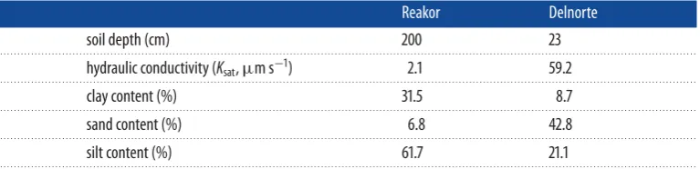
Table 2.Soil properties for the Delnorte and Reakor association soils. Note that the soil textural percentages do not sum to 100 because gravel and organic content have not been reported.

Reakor Delnorte

soil depth (cm) 200 23

. . . . hydraulic conductivity (Ksat,µm s−1) 2.1 59.2

. . . .

clay content (%) 31.5 8.7

. . . .

sand content (%) 6.8 42.8

. . . .

silt content (%) 61.7 21.1

. . . .

method fails to detect some areas where vegetation patterns are visually identifiable. These include regions where vegetation bands are confined to fingers of a particular soil type that are

260 m in extent, meaning that the pattern cannot be identified as the dominant Fourier mode in any given window. There are also some regions where a pattern can be identified by eye, but is so disordered that it falls below the noise threshold. Approximately 10% of the study area consists of isolated patches of patterning which offer little opportunity to explore spatial variations. Instead, we confine our analysis to the 34% (≈64 km2_{) of the image that consists of spatially connected} vegetation patterns. Within these regions, the pattern has a mean wavelength ofλ¯=63±14 m (reported variations are standard deviation unless otherwise specified) and an autocorrelation length of approximately 800 m (i.e.≈12λ). The probability distribution function (PDF) ofΘ(x,y) values is peaked in the north–south direction, but spans a full 0≤Θ < π range.Table 1provides summary statistics describing the average pattern characteristics and topography.

While seven distinct soil types occur in the study area, two of these, the Delnorte and Reakor associations, contain 97% of the vegetation patterning. These soils are distinguished by a relatively low clay and high silt content. The Delnorte association is characterized by a very shallow soil depth (23 cm) due to the presence of calcium-carbonate-based hardpan or petrocalcic horizon. By contrast, Reakor association soils are at least 2 m deep. The full range of soil properties is shown intable 2.

9

rsta.r

oy

alsociet

ypublishing

.or

g

Phil

Tra

ns

R

Soc

A

37

1:

2012035

9

...

slope gradient (%)

P

(

D

Q

) (rad

–1)

DQ (rad)

l

(m)

l (m)

P

(

l

) (m

–1)

(b) (c)

(a)

Reakor Delnorte 4

100

0.03

0.02

0.01

0 60

20 3

2

1

0.3 0.6 0.9 1.2 20 70 120 0

0 p/8 p/4 3p/8 p/2

Figure 3.(a) Frequency distribution ofΘ, the deviation between the local pattern orientation and the local topographic orientation. The slope orientations deviate by less thanπ/8 for 80% of the pattern. (b) Comparison of the local pattern wavelengthλto the local topographic slope. Data were collected into 10 bins of equal size (≈11 000 data points per bin). The box and whisker plots indicate the median (central lines); the 25th and 75th quartiles (box limits) within the bin. The whiskers extend two inter-quartile ranges from the median. The thick line indicates a linear fit to the medians. (c) PDFs of the pattern wavelengths associated with the two major soil classes, indicating the bimodality inλon Reakor association soils. (Online version in colour.)

Table 3.Pattern characteristics comparing analysis of natural and simulated data for a 500×800 m2region. The simulated data come from a modified Rietkirk model calibrated to match the mean pattern properties of the natural data.

mean s.d. corr. length (m) natural pattern wavelengthλ¯(m) 53 4.1 350

. . . . model pattern wavelengthλ¯(m) 54 1.7 360

. . . . natural pattern orientationΘ¯(rad) 1.7 0.39 420

. . . . model pattern orientationΘ¯ (rad) 1.6 0.07 390

. . . . hillslope orientation (rad) 1.7 0.5 120

. . . .

(b) Comparison to model

The results are shown in table 3. We find that while the mean properties of the model and observed pattern are similar (a consequence of calibrating the model to these means),Θandλ vary three to five times more in the observed pattern than in the modelled pattern. The underlying topography is still more variable, and presumably causes the variability of the observed pattern. Thus, even in the region of the study site with the greatest uniformity in the pattern properties, the spatial heterogeneity observed in the real patterns exceeded the pattern variability that could be produced by a physical model. These results justify our attribution of the remaining variability in the pattern properties across the site to environmental variation rather than to defects or initial condition effects arising from the nonlinear dynamics of the system.

(c) Non-uniqueness in pattern attributes

10

rsta.r

oy

alsociet

ypublishing

.or

g

Phil

Tra

ns

R

Soc

A

37

1:

2012035

9

...

(a)

(d)

(b)

(c)

1200 m

700 m

600 m

stream

pattern direction slope direction

ridge

soil type

road

stream Reakor

Delnorte

Q_Q: 0.8 – 1.0

Q_Q: 0.6 – 0.8

Q_Q: 0 – 0.6

1000 m

ridge

Figure 4.Spatial distribution of the uniqueness metricQΘfor the pattern orientation, and magnified cases illustrating different

examples of non-uniqueness in the pattern orientation. (a) Non-uniqueness in orientation associated with a road, which adds north–south oriented structure to the local northeast–southwest oriented banding due to upslope ponding of runoff. (b) A region of changing pattern orientation and wavelength associated with the interleaving of two contrasting soil types. (c) The short length scales on which the pattern can change orientation as it bends around a sharp ridge. A proportion of the region whereΘ≈π/4, as indicated by the different director arrows, hasQΘ>0.75. (d) The deviation between pattern and slope

orientation around a stream channel; again there are regions whereΘ≈π/2 andQΘ>0.75. (Online version in colour.)

11

rsta.r

oy

alsociet

ypublishing

.or

g

Phil

Tra

ns

R

Soc

A

37

1:

2012035

9

...

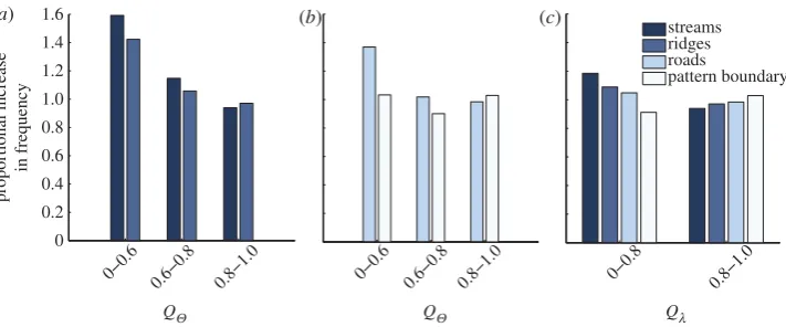
0−0.8 _0.8−1.0 0−0.6 _{0.6−0.8 0.8−1.0} 0−0.6 _{0.6−0.8 0.8−1.0}

0 0.2 0.4 0.6 0.8 1.0 1.2 1.4 1.6

Q_Q Q_Q Q_l

streams ridges roads

pattern boundary

(a) (b) (c)

proportional increase

in frequency

Figure 5.Relative increase in frequency of (a,b) non-unique pattern orientations and (c) wavelengths, for windows within 250 m of local elevation minima (streams), maxima (ridges), roads, and pattern boundaries. All frequencies are measured relative to the frequency in the remainder of the pattern. Non-unique orientations, for example, occurred 50–60% more often near streamlines and ridges than in the bulk of the pattern. (Online version in colour.)

The insets infigure 4illustrate regions of complexity inΘ(x,y).Figure 4a,bshows regions of non-unique pattern directions. Infigure 4a, we show a perturbation of the local pattern by a road. As illustrated, the upslope edge of roads is globally associated with increased vegetation, while the downslope edges are typically bare. Roads thus generate linear features that can create non-uniqueness in the local pattern orientation.Figure 4aalso shows a second anthropogenic feature, a storm drainage outlet, which further decreasesQΘ west of the road.Figure 4billustrates how changes in soil type can lead to lowQΘ. In this example, fingers of the Reakor association soils are interleaved with the Delnorte association soils, causing rapid changes in pattern wavelength and orientation, and consequently multiple energetic values ofθ andkwithin the 260 m windows. Figure 4c illustrates a region where the pattern orientation changes rapidly, turning through approximately π rad within a single 260 m window. Such rapid change inevitably leads to low QΘ because there are multiple pattern orientations located in a single window. There are also, however, regions near the ridge crest where QΘ≈1 and the pattern is locally oriented perpendicular to the slope. Figure 4d is representative of the complex vegetation transitions that occur near stream channels. Here, too, the pattern lies perpendicular to the local hillslope orientation, and rather than curving into the streamline, remains broadly aligned with the band orientation away from the stream.

(d) Soil-type effects

12

rsta.r

oy

alsociet

ypublishing

.or

g

Phil

Tra

ns

R

Soc

A

37

1:

2012035

9

...

200 400 600 800 1000 1200

0 20 40 60 80 100 120

wavelength (m)

200 400 600 800 1000 1200

0 20 40 60 80 100 120

500 1000 1500

0 0.5 1.0 1.5 2.0 2.5

P

(distance ×10

−3

)

500 1000 1500

0 0.5 1.0 1.5

distance from stream (m) distance from stream (m)

(b) (a)

(c) (d)

Figure 6.Distribution of the soils within the pattern-forming areas with respect to landscape position, referenced to the nearest stream channel or local elevation minimum for (a) Reakor and (b) Delnorte association soils. Although both soil types occur across the range of landscape positions, the Reakor association soils are more strongly associated with riparian areas. Distribution of pattern wavelengths on the (c) Reakor association and (d) Delnorte association soils with respect to the nearest stream, again based on equally sized bins of the dataset. There is a strong (r2_{=0.96) and significant (}

p<5×10−7_{) decline in the} wavelength on Reakor soils when moving from the riparian areas to the uplands. There is no correlation between landscape position and pattern properties on the Delnorte association (r2_{=0.08 and}

p=0.4). (Online version in colour.)

4. Discussion

The local Fourier metrics confirm Hypothesis 1 by showing that the wavelength and orientation of the vegetation patterns are typically coherent on scales of 600–800 m, but can change on scales of

≈20 m when the slope orientation changes over the same scale. We were unable to reproduce the observed variation with a model even within regions of relatively uniform patterning, confirming Hypothesis 3 and further suggesting that exogenous factors rather than the pattern-forming mechanisms drive the spatial variability inλandΘ. In the light of these findings, and to address Hypothesis 2, our subsequent analysis focuses on the relationship between exogenous factors and the local pattern properties.

13

rsta.r

oy

alsociet

ypublishing

.or

g

Phil

Tra

ns

R

Soc

A

37

1:

2012035

9

...

Several of these relationships support previous observations. The average hillslope gradient of 0.7% at the Fort Stockton site conforms to observations and predictions of a minimum hillslope gradient being needed for band formation [41], and exceeds the minimum slope gradient observed in other settings (e.g. 0.25% in the Sudan [30]). In addition, the inverse relationship between pattern wavelength and the hillslope gradient (see figure 3) has been identified elsewhere [30,64–66]. However, the one model [67] that has been used to study wavelength– gradient correlations predicts theoppositetrend: steepness causes larger wavelengths [41,68]. We explored this trend with a different model [1] and find that it also produces the opposite trend to that observed in natural systems. While both models predict that multiple pattern wavelengths are stable for a given hillslope gradient [33,69], the selection of particular longer or shorter wavelengths within that range is clearly at odds with observations.

The close correspondence between hillslope and pattern orientation at the Fort Stockton site is a near-universal feature of vegetation patterning. The observed deviations generally arise due to local effects that disrupt the pattern, rapidly alter the direction of water flow, or change the strength and/or length scales of the pattern-forming feedbacks.

Pattern disruption is exemplified by the effects of roads (see figure 4a). Roads disconnect upslope and downslope vegetation bands by preventing the redistribution of water. Rapid alteration of the direction of water flow occurs along ridges and stream channels. The pattern near these locations is less likely to have a unique orientation or wavelength than in the mid-slope areas, and is more likely to have a largeΘ. The prominent ridgeline shown infigure 4cis locally surrounded by a region withΘ≈π/2 andQΘ>0.75. This location provides an unambiguous example of a change in pattern orientation near no-flow boundary conditions, as predicted by McGrath et al. [17]. Other ridgelines are associated with largeΘ, but the low QΘ in these locations makes the interpretation of the observedΘambiguous. Methods that identify a truly local metric of pattern properties, instead of the quasi-local metric used here could both help to resolve these ambiguities, and to extend the analysis into patterned areas less than 260 m wide.

Stream channel locations are also associated with rapid, and sometimes discontinuous changes in pattern orientation. Like the ridge shown infigure 4c, the stream channel shown infigure 4d is surrounded by a region whereΘ≈π/2 andQΘ>0.75, i.e. a unique pattern orientation that is perpendicular to the one expected from the slope orientation. There has been little exploration of the interaction of vegetation pattern with stream channels, presumably because the current paradigm of vegetation pattern models offers little reason to think that such interactions would be important. Stream channels occur in locations where surface runoff rapidly flows away and therefore cannot affect vegetation upslope from the channel. However, we find evidence that the distance from a stream channel alters the pattern properties on the Reakor association soil type. On these soils, the pattern wavelength, vegetation cover and disorder increase near the streams. These observations suggest that an additional mechanism could affect the patterning at this study site: for instance, the stream-channel boundary condition propagating back up into the hillslope. We hypothesize that the ultimate cause of the changes in pattern morphology on the Reakor soils lies in the contrast in the soil depth between the Delnorte and Reakor associations: from 23 cm to over 2 m. We are not the first to propose an association between soil depth and the vegetation pattern structure. Depth to a silcrete hardpan is associated with a transition between sharp patterns (shallow hardpan) and diffuse patterns (deep or no hardpan) in Australia [45,70]. Strikingly coherent vegetation bands in Niger occur above a shallow ironstone hardpan [44]. The broad, diffuse banding near Fort Stockton studied by McDonaldet al.[43] occurs on deep clays. McDonaldet al.[43] cited unpublished research claiming that vegetated bands were associated with a local increase in the depth to the hardpan, similar to previous observations of increased vegetation density on deep soils in Australia [71].

14

rsta.r

oy

alsociet

ypublishing

.or

g

Phil

Tra

ns

R

Soc

A

37

1:

2012035

9

...

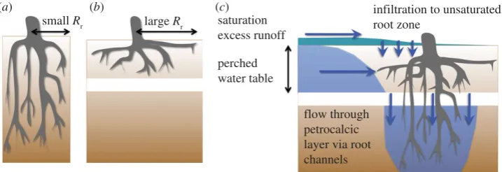
small R_r

(a) (b) (c)

large R_r saturation

excess runoff

perched water table

flow through petrocalcic layer via root channels

infiltration to unsaturated root zone

Figure 7.Schematic of possible effects of a shallow impeding layer on pattern-formation mechanisms. (a) In the absence of an impeding layer, plants develop deep root systems with a smaller lateral root-zone radius,Rr, to exploit water from across the whole soil profile. (b) A shallow impeding layer restricts the vertical growth of roots, confining them to the surface soils, and promoting root competition laterally. (c) The shallow impeding layer also creates the potential for complex subsurface hydrology. Saturation of soils above the impeding layer may promote saturation excess runoff. Gradients—due to changes in the depth of the impeding layer, or in water potential across the impeding layer—can also induce saturated porous media flow. Provided that surface soils near plants can freely drain, the altered hydrology may exaggerate the positive feedback between plants and water. (Online version in colour.)

species confirm that there is intense root competition in the zone above the petrocalcic horizon, where root growth is concentrated [72].

In the second scenario, we recognize that shallow surface soils have limited water storage and saturate readily. For example, the Delnorte association has as little as 2 cm of water storage capacity in the soils above the impeding layer. Unlike dry soils, which only generate runoff during very heavy rains, saturated soils shed all rainfall as runoff. If soils did not saturate near plants this runoff water could be trapped and infiltrate in these locations (figure 7c). Plant roots penetrate and thus may break up hardpans [72]. Root water uptake is also a driver of hardpan formation [73], and hardpans might thus form at greater depth beneath deep-rooted (woody) vegetation. Either mechanism could prevent the surface soil from saturating near the vegetated bands and allow it to store runoff.

The third scenario also relates to the potential for saturation to occur above the hardpan, allowing subsurface saturated flow to occur (figure 7c). The changes in pattern properties with distance to the stream suggest that water availability increases downslope: this requires subsurface storage, if not flow. A relationship between the pattern formation and subsurface flow could explain the local deviations of pattern orientation from slope orientation near the streamlines since the surface orientation might not correspond to the local water table flow direction.

All three scenarios would tend to strengthen the pattern-forming feedbacks on the shallow soils. They could be investigated using subsurface soil moisture sensors to observe shallow soil saturation; water isotope tracers to determine the water sources used by plants; observations of calcium ion concentrations in runoff which would provide an indicator of water contact with the petrocalcic horizon; and root excavations to compare morphologies in sites with different depths to the impeding layer. These studies could be valuable to provide more information about the hydrological role of petrocalcic horizons, which have received relatively little attention given their ubiquity in desert environments [73].

5. Conclusion

15

rsta.r

oy

alsociet

ypublishing

.or

g

Phil

Tra

ns

R

Soc

A

37

1:

2012035

9

...

gradients [30], which are consistent with our observations at local scales. Our analysis shows that while pattern properties mostly vary on scales of 600–800 m, they can change much more rapidly around boundaries in topography or soil characteristics. By analysing the pattern on these fine scales, we identified deviations between hillslope and pattern orientation, soil-controlled changes in pattern wavelength, coherence and vegetation cover, and at least one likely example of the boundary condition effects predicted by McGrath et al. [17]. Two observations, echoed at multiple other sites, are not well explained by current theory: the observation of decreasing pattern wavelength with steepness, and the soil controls on vegetation pattern length scale and coherence.

The large time-scale separation between individual storm events and the time scales on which desert vegetation distributions change mean that an ongoing dialogue between empirical and theoretical studies is critical for understanding the dynamics of these ecosystems. Local information about pattern qualities, when combined with high-resolution information about the pattern substrate, is evidently a useful additional tool for analysis.

Despite the advances in understanding vegetation patterns in the past 10 years, theoretical models still require the use of effective parameters to describe feedbacks, soil–plant–water interactions and the resulting landscape fluxes. Linking theory and observation to make quantitative predictions, therefore, remains an outstanding challenge. Addressing this challenge requires improved observations of within-storm hydrologic processes and plant water use: observations that ecohydrologists are increasingly equipped to make due to developments in distributed sensing systems and tracer technologies. Computational tools for assessing three-dimensional soil moisture dynamics, land–atmosphere interactions and vegetation spread are also improving. By coupling these tools with detailed field measurements, there is potential to develop a detailed theoretical framework that can address the consequences of changing soil depth, root orientation, runoff generation mechanisms and subsurface flow processes on the overall dynamics and resilience of vegetation patterns.

Funding statement. S.E.T. and G.P. acknowledge support from NSF-EAR-1013339.

References

1. Rietkerk M, Boerlijst MC, van Langevelde F, HilleRisLambers R, van de Koppel J, Kumar L, Prins HHT, de Roos AM. 2002 Self-organization of vegetation in arid ecosystems.Am. Nat. 160, 524–530. (doi:10.1086/342078)

2. Thompson S, Daniels K. 2010 A porous convection model for grass patterns.Am. Nat.175, E10–E15. (doi:10.1086/648603)

3. Lefever R, Barbier N, Couteron P, Lejeune O. 2009 Deeply gapped vegetation patterns: on crown/root allometry, criticality and desertification. J. Theoret. Biol. 261, 194–209. (doi:10.1016/j.jtbi.2009.07.030)

4. Pringle RM, Doak DF, Brody AK, Jocqué R, Palmer TM. 2010 Spatial pattern enhances ecosystem functioning in an African savanna. PLoS Biol. 8, e1000377. (doi:10.1371/ journal.pbio.1000377)

5. Borgogno F, D’Odorico P, Laio F, Ridolfi L. 2009 Mathematical models of vegetation pattern formation in ecohydrology.Rev. Geophys.47, RG1005. (doi:10.1029/2007RG000256)

6. Rietkerk M, Dekker S, Wassen M, Verkroost A, Bierkens M. 2004 A putative mechanism for bog patterning.Am. Nat.163, 699–708. (doi:10.1086/383065)

7. Larsen L, Harvey J. 2011 Modeling of hydroecological feedbacks predicts distinct classes of wetland channel pattern and process that influence ecological function and restoration potential.Geomorphology126, 279–296. (doi:10.1016/j.geomorph.2010.03.015)

8. Van de Koppel J, Gascoigne J, Theraulaz G, Rietkerk M, Mooij WM, Herman P. 2008 Experimental evidence for spatial self-organization and its emergent effects in mussel beds. Science322, 739–742. (doi:10.1126/science.1163952)

9. Rietkerk M, Dekker S, de Ruiter P, van de Koppel J. 2004 Self-organized patchiness and catastrophic shifts in ecosystems.Science305, 1926–1929. (doi:10.1126/science.1101867) 10. Scheffer M et al. 2009 Early-warning signals for critical transitions. Nature 461, 53–59.

16

rsta.r

oy

alsociet

ypublishing

.or

g

Phil

Tra

ns

R

Soc

A

37

1:

2012035

9

...

11. Kefi S, Rietkerk M, Alados CL, Pueyo Y, Papanastasis VP, ElAich A, De Ruiter PC. 2007 Spatial vegetation patterns and imminent desertification in Mediterranean arid ecosystems.Nature 449, 213–217. (doi:10.1038/nature06111)

12. Caylor K, Scanlon T, Rodriguez-Iturbe I. 2004 Feasible optimality of vegetation patterns in river basins.Geophys. Res. Lett.31, L13502. (doi:10.1029/2004GL020260)

13. HilleRisLambers R, Rietkerk M, van den Bosch F, Prins HHT, de Kroon H. 2001 Vegetation pattern formation in semi-arid grazing systems. Ecology 82, 50–61. (doi:10.1890/0012-9658(2001)082[0050:VPFISA]2.0.CO;2)

14. Scholes RJ, Archer SR. 1997 Tree-grass interactions in savannas. Annu. Rev. Ecol. Syst. 28, 517–544. (doi:10.1146/annurev.ecolsys.28.1.517)

15. Scanlon TM, Caylor KK, Levin SA, Rodriguez-Iturbe I. 2007 Positive feedbacks promote power-law clustering of Kalahari vegetation.Nature449, 209–212. (doi:10.1038/nature06060) 16. von Hardenberg J, Kletter AY, Yizhaq H, Nathan J, Meron E. 2010 Periodic versus scale-free

patterns in dryland vegetation.Proc. R. Soc. B277, 1771–1776. (doi:10.1098/rspb.2009.2208) 17. McGrath G, Paik K, Hinz C. 2012 Microtopography alters self-organized vegetation patterns

in water-limited ecosystems.J. Geophys. Res.117, G03021. (doi:10.1029/2011JG001870) 18. Thompson SE, Harman CJ, Troch PA, Brooks PD, Sivapalan M. 2011 Scaling of

ecohydrologically mediated water balance partitioning: a synthesis framework for catchment ecohydrology.Water Resour. Res.47, W00J03. (doi:10.1029/2010WR009998)

19. Ravi S, D’Odorico P, Wang L, Collins S. 2008 Form and function of grass ring patterns in arid grasslands: the role of abiotic controls.Oecologia158, 545–555. (doi:10.1007/s00442-008-1164-1) 20. Greene RSB. 1992 Soil physical properties of three geomorphic zones in a semiarid mulga

woodland.Austral. J. Soil Res.30, 55–69. (doi:10.1071/SR9920055)

21. Galle S, Ehrmann M, Peugeot C. 1999 Water balance in a banded vegetation pattern—a case study of tiger bush in western Niger.Catena37, 197–216. (doi:10.1016/S0341-8162(98)90060-1) 22. Harman C, Lohse KA, Troch P, Sivapalan M. Submitted. Co-evolution of resource islands and

microtopography on semi-arid hillslopes.

23. Puigdefábregas J. 2005 The role of vegetation patterns in structuring runoff and sediment fluxes in drylands.Earth Surf. Process. Landforms30, 133–147. (doi:10.1002/esp.1181)

24. Schlesinger WH, Reynolds J, Cunningham G, Huenneke L, Jarrell W, Virginia R, Whitford W. 1990 Biological feedbacks in global desertification. Science 147, 1043–1048. (doi:10.1126/science.247.4946.1043)

25. Gilad E, von Hardenberg J, Provenzale A, Shachak M, Meron E. 2004 Ecosystem engineers: from pattern formation to habitat creation. Phys. Rev. Lett. 93, 098105. (doi:10.1103/ PhysRevLett.93.098105)

26. Yizhaq H, Gilad E, Meron E. 2005 Banded vegetation: biological productivity and resilience. Physica A356, 139–144. (doi:10.1016/j.physa.2005.05.026)

27. Bromley J, Brouwer J, Barker AP, Gaze SR, Valentin C. 1997 The role of surface water redistribution in an area of patterned vegetation in a semi-arid environment, south-west Niger.J. Hydrol.198, 1–29. (doi:10.1016/S0022-1694(96)03322-7)

28. Seghieri J, Galle S, Rajot JL, Ehrmann M. 1997 Relationships between soil moisture and growth of herbaceous plants in a natural vegetation mosaic in Niger. J. Arid Environ.36, 87–102. (doi:10.1006/jare.1996.0195)

29. Barbier N, Couteron P, Lefever R, Deblauwe V, Lejeune O. 2008 Spatial decoupling of facilitation and competition at the origin of gapped vegetation patterns.Ecology89, 1521–1531. (doi:10.1890/07-0365.1)

30. Deblauwe V, Couteron P, Lejeune O, Bogaert J, Barbier N. 2011 Environmental modulation of self-organized periodic vegetation patterns in Sudan.Ecography34, 990–1001. (doi:10.1111/j.1600-0587.2010.06694.x)

31. Meron E, Gilad E, von Hardenberg J, Shachak M, Zarmi Y. 2004 Vegetation patterns along a rainfall gradient.Chaos Solitons Fractals19, 367–376. (doi:10.1016/S0960-0779(03)00049-3) 32. Thompson SE, Katul GG, MacMahon S. 2008 Role of biomass spread in vegetation pattern

formation within arid ecosystems.Water Resour. Res.44, E10421. (doi:10.1029/2008WR006916) 33. Thompson SE, Katul GG. 2009 Secondary seed dispersal and its role in landscape

organization.Geophys. Res. Lett.36, L02402. (doi:10.1029/2008GL036044)

17

rsta.r

oy

alsociet

ypublishing

.or

g

Phil

Tra

ns

R

Soc

A

37

1:

2012035

9

...

35. Konings A, Dekker S, Rietkerk M, Katul G. 2011 Drought sensitivity of patterned vegetation determined by rainfall-land surface feedbacks. J. Geophys. Res. 116, G04008. (doi:10.1029/2011JG001748)

36. Cross MC, Hohenberg PC. 1993 Pattern formation out of equilibrium. Rev. Mod. Phys. 65, 851–1112. (doi:10.1103/RevModPhys.65.851)

37. Lowe M, Gollub J, Lubensky T. 1983 Commensurate and incommensurate structures in a nonequilibrium system.Phys. Rev. Lett.51, 786–789. (doi:10.1103/PhysRevLett.51.786) 38. Eckhaus W, Kuske R. 1997 Pattern formation in systems with slowly varying geometry.SIAM

J. Appl. Math.57, 112–152. (doi:10.1137/S0036139994277531)

39. Hu Y, Ecke R, Ahlers G. 1993 Convection near threshold for Prandtl numbers near 1.Phys. Rev. E48, 4399–4413. (doi:10.1103/PhysRevE.48.4399)

40. Lindner B. 2004 Effects of noise in excitable systems.Phys. Rep.392, 321–424. (doi:10.1016/ j.physrep.2003.10.015)

41. Ursino N, Contarini S. 2006 Stability of banded vegetation patterns under seasonal rainfall and limited soil moisture storage capacity. Adv. Water Resour. 29, 1556–1564. (doi:10.1016/j.advwatres.2005.11.006)

42. Thiéry J, D’Herbès J, Valentin C. 1995 A model simulating the genesis of banded vegetation patterns in Niger.J. Ecol.83, 497–507. (doi:10.2307/2261602)

43. McDonald A, Kinucan R, Loomis L. 2008 Ecohydrological interactions within banded vegetation in the northeastern Chihuahuan Desert, USA.Ecohydrology2, 66–71. (doi:10.1002/ eco.40)

44. White L. 1970 Brousse tigrée patterns in southern Niger.J. Ecol.58, 549–553. (doi:10.2307/ 2258290)

45. Mabbutt J, Fanning P. 1987 Vegetation banding in arid Western Australia.J. Arid Environ.12, 41–59.

46. Macfadyen W. 1950 Vegetation patterns in the semi-desert plains of British Somaliland. Geograph. J.116, 199–211.

47. Worrall G. 1960 Tree patterns in the Sudan. J. Soil Sci.11, 63–67. (doi:10.1111/j.1365-2389. 1960.tb02202.x)

48. Couteron P, Lejeune O. 2001 Periodic spotted patterns in semi-arid vegetation explained by a propagation-inhibition model.J. Ecol.89, 616–628. (doi:10.1046/j.0022-0477.2001.00588.x) 49. Deblauwe V, Couteron P, Bogaert J, Barbier N. 2012 Determinants and dynamics of banded

vegetation pattern migration in arid climates.Ecol. Monogr.82, 3–21. (doi:10.1890/11-0362.1) 50. Cross M, Greenside H. 2009 Pattern formation and dynamics in nonequilibrium systems, 1st

edn, pp. 279–309. Cambridge, UK: Cambridge University Press.

51. National Climatic Data Center. 2010Fort Stockton climate annual summary. Seehttp://www. ncdc.noaa.gov/cdo-web/datasets/ANNUAL/locations/ZIP:79735/detail.

52. National Agricultural Imaging Program. 2010 Pecos county. See http://gis.apfo.usda.gov/ arcgis/services.

53. Richards J. 1999 Remote sensing digital image analysis, 2nd edn, pp. 185–189. Berlin, Germany: Springer.

54. Allen J, Rabiner L. 1977 A unified approach to short-time Fourier analysis and synthesis.Proc. IEEE65, 1558–1564. (doi:10.1109/PROC.1977.10770)

55. Daubechies I. 1990 The wavelet transform, time-frequency localization and signal analysis. IEEE Trans. Inform. Theory36, 961–1005. (10.1109/18.57199)

56. Heutmaker M, Fraenkel P, Gollub J. 1985 Convection patterns: time evolution of the wave-vector field.Phys. Rev. Lett.54, 1369–1372. (doi:10.1103/PhysRevLett.54.1369)

57. Egolf D. 1998 Importance of local pattern properties in spiral defect chaos.Phys. Rev. Lett.80, 3228–3231. (doi:10.1103/PhysRevLett.80.3228)

58. Daniels KE, Brausch O, Pesch W, Bodenschatz E. 2008 Competition and bistability of ordered undulations and undulation chaos in inclined layer convection.J. Fluid Mech.597, 261–282. (doi:10.1017/S0022112007009615)

59. Pinnegar C, Mansinha L. 2004 Time-local Fourier analysis with a scalable, phase-modulated analyzing function: the s-transform with a complex window.Signal Process.84, 1167–1176. (doi:10.1016/j.sigpro.2004.03.015)

60. Burton GJ, Moorhead IR. 1987 Color and spatial structure in natural scenes.Appl. Opt. 26, 157–170. (doi:10.1364/AO.26.000157)

18

rsta.r

oy

alsociet

ypublishing

.or

g

Phil

Tra

ns

R

Soc

A

37

1:

2012035

9

...

62. Oimoen M. 2000An effective filter for removal of production artifacts in U.S. Geological Survey 7.5 minute digital elevation models. Technical report. Sioux Falls, SD: USGS EROS Data Center. 63. Lefever R, Lejeune O. 1997 On the origin of tiger bush. Bull. Math. Biol. 59, 263–294.

(doi:10.1007/BF02462004)

64. Valentin C, d’Herbes J, Poesen J. 1999 Soil and water components of banded vegetation patterns.Catena37, 1–24. (doi:10.1016/S0341-8162(99)00053-3)

65. d’Herbès J, Valentin C, Tongway D, Leprun J. 2001 Banded vegetation patterns and related structures. InBanded vegetation patterning in arid and semiarid environments: ecological processes and consequences for management(eds D Tongway, C Valentin, J Seghieri). Ecological Studies, vol. 149, pp. 1–19. New York, NY: Springer.

66. Eddy J, Humphreys G, Hart D, Mitchell P, Fanning P. 1999 Vegetation arcs and litter dams: similarities and differences.Catena37, 57–73. (doi:10.1016/S0341-8162(98)00055-1)

67. Klausmeier C. 1999 Regular and irregular patterns in semiarid vegetation. Science 284, 1826–1828. (doi:10.1126/science.284.5421.1826)

68. Sherratt J. 2005 An analysis of vegetation stripe formation in semi-arid landscapes.J. Math. Biol.51, 183–197. (doi:10.1016/j.tpb.2006.07.009)

69. Sherratt J, Lord G. 2007 Nonlinear dynamics and pattern bifurcations in a model for vegetation stripes in semi-arid environments.Theoret. Popul. Biol.71, 1–11. (doi:10.1016/j.tpb.2006.07.009) 70. Tongway DJ, Ludwig JA. 1990 Vegetation and soil patterning in semi-arid mulga lands of

Eastern Australia.Austral. J. Ecol.15, 23–34. (doi:10.1111/j.1442-9993.1990.tb01017.x)

71. Mott J, McComb A. 1974 Patterns in annual vegetation and soil microrelief in arid region of Western Australia.J. Ecol.62, 115–126. (doi:10.2307/2258884)

72. Gibbens R, Lenz J. 2001 Root systems of some Chihuahuan Desert plants.J. Arid Environ.49, 221–263. (doi:10.1006/jare.2000.0784)