Scholarship@Western
Scholarship@Western
Electronic Thesis and Dissertation Repository
12-15-2016 12:00 AM
In Mold Flow of Long Fibers in Compression Molding Process
In Mold Flow of Long Fibers in Compression Molding Process
Gleb Meirson
The University of Western Ontario
Supervisor
Dr. Andrew Hrymak
The University of Western Ontario
Graduate Program in Chemical and Biochemical Engineering
A thesis submitted in partial fulfillment of the requirements for the degree in Doctor of Philosophy
© Gleb Meirson 2016
Follow this and additional works at: https://ir.lib.uwo.ca/etd
Part of the Polymer Science Commons, and the Structural Materials Commons
Recommended Citation Recommended Citation
Meirson, Gleb, "In Mold Flow of Long Fibers in Compression Molding Process" (2016). Electronic Thesis and Dissertation Repository. 4377.
https://ir.lib.uwo.ca/etd/4377
This Dissertation/Thesis is brought to you for free and open access by Scholarship@Western. It has been accepted for inclusion in Electronic Thesis and Dissertation Repository by an authorized administrator of
Abstract
Long Fiber Thermoplastics (LFT) are promising new materials with high physical
properties and low density. These high properties are obtained by embedding very long
fibers (∼100 mm) into a thermoplastic matrix. Such a high fiber length dictates the use
of a compression molding process for manufacturing as the length of discontinuous fibers
in injection molding is limited by pellet length.
LFT composites are of great interest for the automotive industry. These materials
are already used in some interior and exterior car parts such as bumpers, seat structures,
door module etc. This research is inspired by the desire to manufacture load carrying
parts for vehicles such as wheel rims which would dramatically reduce vehicle weight and
subsequently save fuel. This, however, requires a much better understanding of long fiber
orientation and distribution during compression molding.
Current orientation models were developed for short fibers (<1mm). Initially these models were extended to cases that were considered long fibers (several millimetres).
Recently these models are being extended even for the LFT-D case fibers which can
reach up to 80 mm. Since several of the governing assumptions for short fiber models are
not suitable for long fibers, the models can not provide accurate results for long fibers.
Due to this limitation long fibers require independent treatments.
This thesis presents a new model which is specifically designed for long flexible fibers.
This model is confirmed by comparing results obtained for simple shear flow to results
found in the literature. The model was implemented in a rheometric squeeze flow, which
is defined as flow between two approaching to each other parallel plates, and provided
results previously not seen in the literature. Interactions were implemented into the
model and tested for rheometric squeeze flow and simple shear flow cases. In addition to
providing insight into fiber orientation and deformation in rheometric squeeze flow, which
was not previously studied in the literature, the proposed model shows more predictive
results than previously found in the literature.
Keywords: Long fibers, Composite materials, Automotive industry, Fiber
orienta-tion, Compression molding, Injection molding.
I would like to thank Ontario Trillium Scholarship, Ontario Research Fund and
Gen-eral Motors Canada for funding this project.
I express my sincere gratitude to my supervisor Dr. Andrew Hrymak, for his constant
guidance and encouragement. During the past four and a half years he became my
super-visor, mentor and friend. I would also like to thank my committee members Dr. David
Jeffrey and Dr. Ajay Ray for their time and advice.
I am very grateful for the support of CBE administrative staff, my group mates, office
mates and my friends on the department and especially my dear friend Stanislav Ivanov
for their support.
I would like to acknowledge the Western SHARCNET team and especially Ge Baolai
for helping me to run my simulations on their system.
Last but not least, I would like to thank my amazing family. My parents who sacrificed
their desires so that their children could have a better life, my brother whom I can always
count for a wise advice and my beautiful wife who was always there for me in the past
four and a half years, supported me and helped me when I needed it the most.
Without you all this thesis would not be possible, my sincere thanks to you all. You
will forever be in my heart.
Contents
Abstract i
Acknowlegements ii
List of Figures vi
List of Tables xi
List of Appendices xii
1 Introduction 1
1.1 Composites History . . . 1
1.2 Long Fiber Thermoplastic Composites . . . 1
1.3 Orientation Models . . . 4
1.3.1 Single Short Rigid Fiber . . . 4
1.3.2 Short Rigid Fiber Suspensions . . . 9
1.4 Flexible Fibers . . . 15
1.4.1 Orientation Models - Flexible Fiber . . . 15
1.5 Interactions . . . 16
1.5.1 Interaction Between Spheres . . . 17
1.5.2 Interactions Between Fibers . . . 18
1.6 Rheology . . . 19
1.6.1 Homogeneous Systems . . . 19
1.6.2 Fiber Filled Systems . . . 21
1.7 Squeeze Flow . . . 22
1.8 Objectives . . . 25
2.1 General Approach . . . 26
2.2 Rigid Cylinder . . . 27
2.2.1 Infinite Axis Ratio Cylinder . . . 27
2.2.2 Finite Axis Ratio Cylinder . . . 32
2.3 Flexible Fiber . . . 35
2.3.1 Elongation . . . 36
2.3.2 Bending . . . 38
2.4 Interactions . . . 43
2.5 Tolerance . . . 44
2.6 Summary . . . 46
3 Simple Shear 48 3.1 Rotational Friction Coefficients . . . 48
3.2 Rigid Cylinder . . . 50
3.3 Flexible Fiber . . . 53
3.4 Calculation time . . . 58
4 Squeeze Flow 60 4.1 Rigid Fiber . . . 64
4.2 Flexible Fiber . . . 67
System A . . . 67
System B . . . 77
5 Interactions 85 5.1 Rigid Cylinders . . . 85
5.2 Flexible Fibers . . . 89
5.2.1 Simple Shear Flow . . . 89
5.2.2 Squeeze Flow . . . 89
6 Conclusions 94 6.1 Simple Shear Flow . . . 94
6.2 Rheometric Squeeze Flow . . . 95
6.3 Interactions . . . 95
6.4 Future Work . . . 96
Bibliography 98
A Squeeze Flow Fiber Orientation 111
Curriculum Vitae 117
1.1 LFT-D brick. . . 2
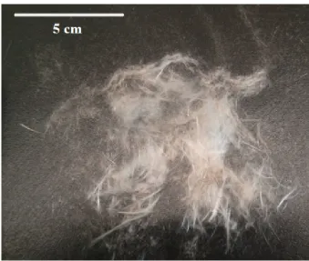
1.2 Fibers after a burn test from LFT-D charge. . . 2
1.3 Composite properties as a function of fiber length [5-7]. . . 3
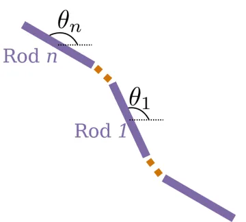
1.4 Representation of fiber on axes . . . 5
1.5 Graphical θ representation. . . 6
1.6 Ellipsoid’s reaction to simple shear flow with shear rate ˙γ = 4s−1. Upper case is for ellipsoid of infinite axis ratio and the bottom case is for axis ratio of 5. . . 7
1.7 Two dimensional orientation tensor representation. . . 11
1.8 Different groups of fiber deformations in simple shear flow [63]; a)axial spin, b)flexible spin, c)springy rotation, d)snake turn, e)S-turn. . . 14
1.9 Lubrication forces. . . 18
1.10 Squeeze flow system. . . 24
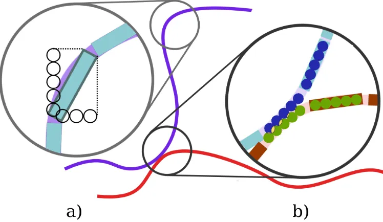
2.1 Graphic model representation;a) Cylinder is represented through projec-tions divided into spheres for hydrodynamic torque and force calculation. b) Cylinder is represented through a collection of spheres for interactions calculations. . . 27
2.2 Comparison between Jeffery’s model and current model for the case of constant friction coefficient in interval [π/2,0]. . . 30
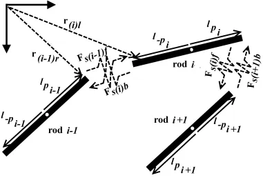
2.3 Superposition of forces on the cylinder. . . 32
2.4 a. Representation of a cylinder through a collection of spheres on the cylinder projections. b. Representation of cylinder’s cross section with two spheres. . . 33
2.5 Cross section projections change during orientation. . . 34
2.6 Schematic representation of rigid segments connected through elastic springs. 36 2.7 Elongation diagram. . . 37
2.8 Bending diagram. . . 39
2.9 Schematic representation of bending torque with imeginary force Fbp. . . 40
2.10 Schematic representation of elastic collision force. . . 44
2.11 Cycle times of rigid fiber of axis ratio of 40 solved for two different tolerances. 45 3.1 Comparison between simulation and Jeffery’s model solution for the fol-lowing conditions: dl =∞,γ˙ = 41s,l = 0.001. . . 50
3.2 Comparison between simulation and Jeffery’s model solution for the fol-lowing conditions: dl = 5 (4.3 equivalent), ˙γ = 41s,l = 0.001m. . . 51
3.3 Friction coefficients as a function of shear rate. . . 51
3.4 Comparison between simulation and experimental [34] periods of rotation of a rigid fiber as a function of aspect ratio. . . 52
3.5 Flexible fiber transition states through rotation in a simple shear flow ˙ γ = 41s. The flow is from left to right. . . 54
3.6 Graphical representation of bending parameter. . . 55
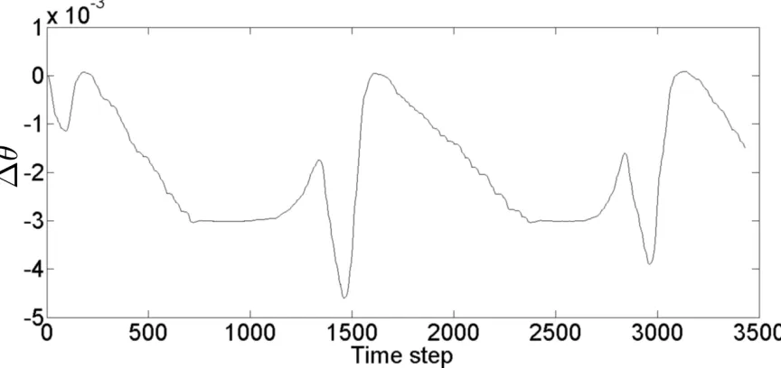
3.7 ∆θ calculations for the E = 109P a case from Figure 3.5. . . . 55
3.8 ∆θ calculations for the E = 1010P a case from Figure 3.5. . . . 56
3.9 Comparison between theoretical [31] and simulated values for critical Young modulus values for buckling. . . 57
3.10 12 mm fiber made out of rigid parts with axis ratio of 4,5 and 6 with Young’s modulus of 108P aat shear rate of 4s−1. . . 57
3.11 12 mm fiber made out of rigid parts with axis ratio of 4,5 and 6 with Young’s modulus of 109P aat shear rate of 4s−1. . . . 58
4.1 Upper plate velocity as a function of time. . . 62
4.2 Upper plate location as a function of time. . . 63
4.3 Solution of a squeeze flow system (for system A). . . 63
squeeze flow. Fiber initial coordinates are (xo, yo) = (0.8,0.8). . . 65
4.5 Solution of Jeffery’s model for a fiber at different initial coordinates for λ= 1. . . 65
4.6 Comparison between simulation and Jeffery’s model solution for: dl =∞, l= 1mm. . . 66
4.7 Comparison between simulation and Jeffery’s model solution for: dl = 5, l= 1mm. . . 66
4.8 Path of fiber’s center mass from Figures 4.9-4.20. . . 68
4.9 Fiber orientation and deformation in squeeze flow for three values of Young’s modulus A.109P a, B.108P a and C.107P a for fiber placed at the initial position of (x/c, y/a0) = (0.8,0.8) using coordinates of Figure 1.10. The fiber is presented at times: 0, 2.37, 5.54, 8.13 and 8.8 s. . . 69
4.10 Fiber orientation and deformation in squeeze flow for three values of Young’s modulus A.109P a, B.108P a and C.107P a for fiber placed at the initial position of (x/c, y/a0) = (0.8,0.4) using coordinates of Figure 1.10. The fiber is presented at times: 0, 2.37, 5.54, 8.13 and 8.8 s. . . 70
4.11 Shear rate in system A at time t= 0. . . 72
4.12 Shear rate in system A at time t= 5. . . 73
4.13 Shear rate in system A at time t= 9. . . 73
4.14 Fiber orientation and deformation in squeeze flow for three values of Young’s modulus A.109P a, B.108P a and C.107P a for fiber placed at the initial position of (x/c, y/a0) = (0.8,0) using coordinates of Figure 1.10. The fiber is presented at times: 0, 2.37, 5.54, 8.13 and 8.8 s. . . 74
4.15 Fiber orientation and deformation in squeeze flow for three values of Young’s modulusA.109P a, B.108P aandC.107P afor fiber that was placed at the initial position of (x/c, y/a0) = (0.8,0.003) using coordinates of Fig-ure 1.10.The fiber is presented at times: 0, 2.37, 5.54, 8.13 and 8.8 s. . . 75
4.16 Fiber orientation and deformation in squeeze flow for Young’s modulus of
107P a. The fiber is placed with center mass at (x/c, y/a
0) = (0.8,0.8) at
three different initial orientations: A.−0.2π, B.−0.3π, C.−0.4π.The fiber is presented at times: 0, 2.37, 5.54, 8.13, 8.8 and 9.2 s. . . 76
4.17 Fiber orientation and deformation in squeeze flow for three values of
Young’s modulus A.109P a, B.108P a and C.107P a for fiber placed at the initial position of (x/c, y/a0) = (0.8,0.8). The fiber is presented at times:
0, 2.37, 5.54, 8.13 and 8.8 s. . . 78
4.18 Fiber orientation and deformation in squeeze flow for three values of
Young’s modulus A.109P a, B.108P a and C.107P a for fiber placed at the
initial position of (x/c, y/a0) = (0.8,0.4). The fiber is presented at times:
0, 2.37, 5.54, 8.13 and 8.8 s. . . 79
4.19 Fiber orientation and deformation in squeeze flow for three values of
Young’s modulus A.109P a, B.108P a and C.107P a for fiber placed at the
initial position of (x/c, y/a0) = (0.8,0). The fiber is presented at times:
0, 2.37, 5.54, 8.13 and 8.8 s. . . 81
4.20 Fiber orientation and deformation in squeeze flow for three values of
Young’s modulus A.109P a, B.108P a and C.107P a for fiber placed at the initial position of (x/c, y/a0) = (0.8,0.03). The fiber is presented at times:
0, 2.37, 5.54, 8.13 and 8.8 s. . . 82
4.21 Fiber orientation and deformation in squeeze flow for three Young’s
mod-ulus 107P a placed at initial position (x/c, y/a) = (0.8,0.8) in system A,
with flow parameterR= 0.1. Thefiber is shown at time:0, 1.13, 2.75, 4.07, 4.34 s. . . 83 5.1 Interactions between rigid cylinders at shear rate of ˙γ = 41s. . . 87 5.2 Normalised rotation time with dependence to ratio of length of cylinders
to initial distance between cylinders centers of mass. . . 88
5.3 Interactions between 8mmflexible fibers placed in initial distance of 4mm
start perpendicular position to each other. . . 92
5.5 Interactions between two flexible fibers in squeeze flow where the fibers start at an angle of 5/6π angle to each other. . . 93
A.1 Rheology results of petroleum jelly at 22◦C. . . 112
A.2 Fiber Young’s modulus measurement. . . 112
A.3 Visualization experiment, resulting fiber shape at 3.3s. . . 114
A.4 Long flexible fiber simulation in power law fluid, experimental viscosity. . 115
A.5 Long flexible fiber simulation in power law fluid, literature viscosity. . . . 116
List of Tables
2.1 Physical properties in the system . . . 47
2.2 Calculated properties in the system . . . 47
2.3 Model parameters in the system . . . 47
3.1 Friction coefficient parameters for several cylinder dimensions. . . 50
3.2 Number of simulation steps and simulation time for various fibers simula-tions (initial position of fiber’s center of mass was at [0.8, 0.8] . . . 59
4.1 System’s A and B parameters. . . 61
Appendix A Squeeze Flow Fiber Orientation . . . 111
Chapter 1
Introduction
1.1
Composites History
A composite is defined as a: ”thing made up of several parts or elements” [1]. The reason
behind creating composites is making a material whose combined physical properties are
superior to the physical properties of its components.
Composites were known to mankind for thousands of years. The first recorded case of
composite use was around 3200 B.C. in Mesopotamia when they combined wood stripes
at different angles to create a material with better properties. Structures found in Egypt
and Mesopotamia dated 1500 B.C were built of mud bricks, which contained straw for
reinforcement [2].
Using composites presents a great opportunity to reduce structure weight while at the
same time not compromising reliability. For example, plastic reinforced by 50% volume
of high modulus continuous graphite fibers has five times greater modulus of elasticity
and tensile strength per weight than steel [3].
1.2
Long Fiber Thermoplastic Composites
Thermoplastic composites saw a great increase in production in the 1960s, due to the
development of carbon fibers, which significantly increased the stiffness of the composite
compared to traditionally used glass fibers [4]. Later it was found that an increase in fiber
length provides enhanced properties to the resulting compound [5–10]. That discovery
opened the door for a new process: Long Fiber Thermoplastic (LFT).
LFT process was commercialized in the mid to late 90s [11]. The fibers were
embed-ded into the polymer, which was then cut to produce pellets of neeembed-ded length. These
pellets were then injected or compressed into a mold. As a result, the fibers embedded in
the final product were longer than previous composites produced, but still relatively short
Figure 1.1: LFT-D brick.
1.2. Long Fiber Thermoplastic Composites 3
Figure 1.3: Composite properties as a function of fiber length [5-7].
due to limitations on the pellet size. Fibers longer than 1 mm are considered long [12]
by injection molding standards. Recently a new process Long Fiber Thermoplastic-
Di-rect (LFT-D) started to gain momentum. LFT-D process consists of two continuously
operated twin screw extruders and a press. The first extruder mixes the polymer with
additives (antioxidants, color etc.) and feeds the melt into the second extruder, which
pulls and mixes continuous fibers, that may be broken during the mixing process, with
the melt. The second extruder has a rectangular die which produces a brick shaped
compound (Figure 1.1) of polymer and long fibers (up to 80 mm) as seen in Figure 1.2.
The sample was obtained by a burn test which was made by burning part of the brick
thus removing the polymeric matrix and exposing the fibers. This brick is then placed
into a press and pressed into the final product. The main advantages of this new process
are due to improved composite properties by increasing the fiber length, and
improv-ing manufacturimprov-ing logistics [13]. The improvement in composite properties versus fiber
length could be observed in Figure 1.3. Fiber orientation is a highly influential factor
on composite properties. Composites are particularly strong in the direction in which
the fibers are aligned. It has also been found that increasing waviness of fibers in the
affect both the material micro-structure and properties [15]. Hence it is highly important
to study the dynamics of fiber orientation in composite manufacturing process. Current
fiber orientation models which will be described in the next sections of this chapter are
designed for short fibers and hence can not accurately predict long fiber orientation. Due
to that it is required to develop a new model which is specifically designed for long fibers.
1.3
Orientation Models
1.3.1
Single Short Rigid Fiber
Jeffery [16] analytically solved the equations of motion for short ellipsoid particle in
low Reynolds number flow, thus predicting its orientation under the influence of a flow
field [16], and predicts an ellipsoid’s response to Stokes drag [17]. Jeffery’s model is
limited by a number of assumptions [16]:
i. The particle is of ellipsoid shape.
ii. The flow is considered non-inertial, which implies a low Reynolds (Re) number
(Re1).
iii. Particle dimensions are small compared to dimensions of the system.
iv. The center mass of the fiber is at rest with respect to the flow, i.e. the particle is
moving with the velocity of the flow.
v. The particle is rigid.
vi. The model is developed for a particle placed in a Newtonian fluid.
Jeffery [16] derived his model for a general flow, then simplified it for a simple shear
flow case, and obtained the following equation for a three dimensional ellipsoid under the
influence of a simple shear flow:
dϕ dt =
˙
γ
(A.R2+ 1) A.R 2
1.3. Orientation Models 5
(1.1)
dβ dt =
˙
γ(A.R2 −1)
4 (A.R2+ 1) sin (2β) sin (2ϕ), (1.2)
where β and ϕ(Figure 1.4) are angles between the ellipsoid and the axes (as shown in Figure 1.4),A.R is the axis ratio defined as length divided by diameter, ˙γ is the local shear rate which in a simple shear flow could be defined as a derivetive of velocity in the
direction in which the velocity is changing. It could be seen that for the case where the
axis ratio is equal to infinity, meaning the ellipsoid is infinitely long or infinitely thin,
the ellipsoid will orient itself with the flow while for the case of a finite axis ratio, the
ellipsoid will rotate. For the case of a simple shear flow (eqs. (1.1)-(1.2)) Jeffery’s model
could be analytically solved and the solution for angles (β,ϕ) and period of rotation T are presented in eqs.(1.3)-(1.5) [16]:
tan(ϕ) = A.R·tan2πt
T
(1.3)
tan(β) = C·A.R
(A.R2cos2(ϕ) + sin2(ϕ))0.5 (1.4)
T =
2π
˙
γ A.R+
1
A.R
(1.5)
Sometimes it is enough to solve the two dimensional case; for example, a simple
shear case where the ellipsoid is lying in the x−y plane (essentially 2-D case). For these simplified cases, Jeffery’s model in its general form could be presented through
eq. (1.6) [18]:
dθ dt =
A.R2
A.R2 + 1 −sin (θ) cos (θ)
∂vx
∂x −sin
2(θ)∂vx
∂y +cos
2(θ)∂vy
∂x + sin (θ) cos (θ) ∂vy ∂y − 1
A.R2+ 1 −sin (θ) cos (θ)
∂vx
∂x +cos
2(θ)∂vx
∂y −sin
2(θ)∂vy
∂x + sin (θ) cos(θ) ∂vy
∂y
(1.6)
Angle θ is represented in Figure 1.5 and the solutions of this equation for ellipsoids with axis ratio of infinity and five (5) placed in a simple shear flow field with shear rate
of 4s−1 are presented in Figure 1.6 in both cases ellipsoid is initially oriented in the y
direction:
In the mid-80s an orientation vector form of Jeffery’s model started to appear in the
scientific literature [19, 20].
Three dimensional ellipsoidal particle orientation could be described through the
ori-entation vectorp= [px, py, pz] (shown in Figure 1.4). The general vector form of Jeffery’s
1.3. Orientation Models 7
Figure 1.6: Ellipsoid’s reaction to simple shear flow with shear rate ˙γ = 4s−1. Upper
case is for ellipsoid of infinite axis ratio and the bottom case is for axis ratio of 5.
model could be expressed through eq. (1.7) [21]:
dp
dt =σ·p+λ D·p− p
T·
D·pp, (1.7) whereσ is a vorticity tensor,D is the deformation tensor andλis a function of axis ratio
A.R.
σ= 0.5 L−LT
(1.8)
D= 0.5 L+LT (1.9)
L= dvx dx dvy dy dvz dz dvx dy dvy dy dvz dy dvx dz dvy dz dvz dz (1.10)
λ= A.R
2−1
Multiple experimental works confirmed Jeffery’s results [22–27]. It was found that
Jeffery’s model could be applied not only for ellipsoids, but also to cylinders, as long as
equivalent axis ratio A.Re is used to describe the geometry of the cylinder. Equivalent
axis ratio of a cylinderA.Re is smaller than its real axis ratioA.Rand it is essentially the
axis ratio of a corresponding ellipsoid that will exhibit the same response to a flow field
as the cylinder with the corresponding axis ratio A.R. Thus Jeffery’s model could be used to simulate rod-like fiber behaviour under the influence of a flow field [23,24,28–30].
Experimental data for these measurements is found in several works [23, 25, 31–34]. Cox
[35] developed an analytical expression for forces acting on a slender body by the fluid
and compared the results for a cylinder and ellipsoid.
F1 =
2πµlU
ln (2l/d) +OI
, (1.12)
OI =
−1 2 + 1 4 +1 Z −1 ln
1−s2
Λ2
ds, (1.13)
where µ is viscosity of the fluid,l is particle’s length, d is particle’s diameter, U is fluid velocity,sis dimensionless distance between the center and the ends of the particle and Λ is a dimensionless function of cross-sectional radius of an arbitrary geometric at any point
along its major axis. Thus for a cylinder, Λ = 1, while for an ellipsoid Λ = (1−s2)0.5 where s is a dimensionless coordinate on the major axis defined as −1 < s < 1. For a cylinder, OI =−1.5 +ln2 while for the ellipsoid OI =−0.5.
Cox [36] noticed that for the ratio of cases of θ= π2 and θ = 0, the expression (1.14) for equivalent axis ratio will be generated:
ωθ=0
ωθπ2
=A.R2e, (1.14)
where ωθ=0 is radial velocity of rod in a position of θ = 0 and ωθπ2 is radial velocity of
rod in a position of θ= π
2, for the case of an ellipsoid A.Re =A.R.
Hence by measuring the radial velocity of a cylinder at a vertical and horizontal position,
1.3. Orientation Models 9
radial velocity, Cox took it one step further and assumed that since radial velocity is
proportional to torque it could be said that:
A.Re =
rω
θ=0
ωθπ2
=
s
Pθ=0
Pθπ2
(1.15)
where Pθ=0 is torque acting on a rod oriented in the direction of θ = 0 and Pθπ2 is the
torque acting on a rod oriented in the direction of θ = π2. Cox then uses the derivation of forces acting on a slender body [35] to calculate Pθ=0 and derives the expression of
Pθπ2 [36]. By dividing these two expressions, Cox [36] found an expression for equivalent
axis ratio:
A.Re
A.R =
8π
3L
!0.5
ln(A.R)−0.5, (1.16) where L is a constant fitted to be 5.45 from the experimental data of cylinder axis ratio
compared to equivalent axis ratio [25].
Harris and Pittman [37] fitted a model to match the experimental results. Eq. (1.17)
provides a good fit in the range of 50< A.R <450 (error is within ±5% )
A.Re= 1.14A.R0.844 (1.17)
Zhang et. al. [38] developed a finite element method (FEM) to simulate the movement
of a single fiber in a general flow field and compared it to Jeffery’s model solution as well
as computationally finding equivalent axis ratio for several axis ratio cylinders.
Although Jeffery’s model was developed in 1922 and has many limiting assumptions
it is still widely used [21, 39, 40]
1.3.2
Short Rigid Fiber Suspensions
Rod like fiber suspension behaviour and properties are highly dependent on fiber
concen-tration and was widely investigated [41–44]. It is common to divide the volume fraction,
ii. Semi-concentrated: dl2 < c < dl -the distance between the neighboring fibers is less than l but greater than d.
iii. Concentrated: dl < c -the distance between the neighbouring fibers is less than d. Where d is the fiber diameter and l is the fiber length. As the distance between the fibers becomes less thanl, they can no longer rotate freely and start to interact with each other thus contradicting Jeffery’s assumptions. These interactions have to be accounted
for in order to accurately predict the orientation.
In order to account for interactions, Folgar and Tucker [18] added a rotational diffusion
term to Jeffery’s model and assumed infinite aspect ratio A.R thus creating the following
model:
dθ
dt =−sin (θ) cos (θ) ∂vx
∂x −sin
2(θ)∂vx
∂y +cos
2(θ)∂vy
∂x + sin (θ) cos (θ) ∂vy
∂y − CIγ˙
ψθ
∂ψθ
∂θ ,
(1.18)
where vx is the fluid velocity in the direction of x, vy is the fluid velocity in the y
direction, CI is the interaction coefficient, ψθ is the density distribution function of fiber
orientation and ˙γ is scalar value of a shear rate. Advani and Tucker [45] defined a second order orientation tensor a through the orientation distribution density function:
a=
Z
p⊗pψ(p)dp (1.19) The trace of a second order orientation tensor is always one, which sometimes makes it
sufficient to track only one of the tensor diagonal values. A two dimensional orientation
tensor meaning is shown in Figure 1.7. The Folgar-Tucker model in its orientation tensor
form is given as:
da
dt = (σ·a−a·σ) +λ(D·a+a·D−2a4 :D) + 2qCIγ˙( I
q −a), (1.20)
where a4 is 4th order orientation tensor, I is identity matrix and q is the problem
di-mension such that for the two didi-mensional case q = 2. Fourth order orientation tensor
1.3. Orientation Models 11
Figure 1.7: Two dimensional orientation tensor representation.
order orientation tensor a, the simplest of these approximations is called the “quadratic approximation” [46, 47]:
a⊗a=a4 (1.21)
Other more complicated approximations can be found in the literature [46,48,49]. Advani
and Tucker [45] solved the Folgar-Tucker model eq. (1.20) for differenta4 approximations.
Bay [50] proposed a correlation for the interaction parameterCI as a function of fiber
volume fractionc and ellipsoid axis ratio A.R:
CI = 0.0184·e−0.714·c·A.R (1.22)
Phan-Thien et al. [51] suggested another correlation for CI:
CI =M 1−e−B·c·A.R
, (1.23)
whereM andB are constants, which were found by comparison to experimental data to be 0.03 and 0.224 respectively.
Ferec et. al. [52] modified the Folgar-Tucker model by replacing the constant
function.
The Folgar-Tucker model is widely used for injection molding simulation of short fiber
composites [53–55].
It was found that systems simulated by the Folgar-Tucker model orient with the
flow faster than what could be seen from experimental results. Huynh [56] found that
experimentally tested injection molded parts were at an orientation level, which required
five to ten times less shear rate than what the Folgar-Tucker model would predict to
require in order to achieve similar orientation level for the same flow time. Huynh added
a parameterH to the Folgar-Tucker model in order to slow the orientation predicted by Folgar-Tucker:
da dt =H
(σ·a−a·σ) +λ(D·a+a·D−2a4 :D) + 2qCIγ˙(
I q −a)
, (1.24) 1/H is the strain reduction factor and is defined between infinity and 1, where the H = 1 corresponds to the Folgar-Tucker model.
Sepehr et al. [57–59] tried to predict the stress in the compression experiment using
the orientation calculated by the Folgar-Tucker model, and like Huynh [56] they found
that the calculated stress diverges from the experimental value. In order to achieve a
match between computational and experimental results they had to use a reduced shear
rate in Folgar-Tucker model calculations.
Although Huynh’s [56] SFR (Strain Factor Reduction) model gives good results in simple
flows, it fails in a general case flow since the results depend on the coordinate system [60].
A more general model (RSC – Reduced Strain Closure) was developed by Wang et. al. [61].
In this model, the growth rate of eigenvalues of the orientation tensor is modified by an
empirical factor k while the rotation rate eigenvectors remain unchanged.
da
dt = (σ·a−a·σ) +λ(D·a+a·D−2[a4+ (1−k)(L4−M4 :a4)] :D) + 2qCIγ˙( I q −a),
(1.25)
1.4. Flexible Fibers 13
eigenvectors ei calculated from the orientation tensor a:
L4 = 3
X
i=1
λieieieiei (1.26)
M4 = 3
X
i=1
eieieiei (1.27)
k- empirical constant≤1, For k = 1 RSC is the Folgar-Tucker model.
The RSC model gives a good prediction for short fiber composites (0.2−0.4mmfibers); however, it fails for longer fibers. Anisotropic Rotary Diffusion (ARD) model [62] was
developed for long fiber injection molding (10−13mmfibers) prediction.
da
dt = (σ·a−a·σ) +λ(D·a+a·D−2[a4+ (1−k)(L4−M4 :a4)] :D)
+2k(trC)a−5 (Ca+aC) + 10 (a4+ (1−k) (L−M :a4)) :C) (1.28)
C- Rotary diffusion tensor
C =b1I+b2a+b3a2+b4
D
˙
γ +b5 D2
˙
γ2, (1.29)
where bi are empirical constants that have to be fitted experimentally.
ARD provides similar results to RSC for short fiber and better prediction for long
fibers. Although the long fiber referred to in regards with ARD are still much shorter
than fibers in the LFT-D process.
Although the fibers described in this section are much shorter than the fibers that are
targeted for this research, the results obtained by the methods described above are still
important. Long fibers could be broken down in to smaller components whose average
1.4. Flexible Fibers 15
1.4
Flexible Fibers
As previously mentioned fiber length in LFT-D material can reach up to 80 mm, which
violate the assumption of short rigid fibers used in Jeffery’s model [16], hence models
that use Jeffery’s model as their base shouldn’t be used to simulate this process. Long
fibers will exhibit bending during the flow. It is important to predict fiber bending in
the composite since the fiber’s shape affects composite properties [14].
Forgacs and Mason [31, 32] and Arlov et. al. [63] experimentally investigated flexible
fiber dynamics under the influence of simple shear flow. They classified the results into
three groups:
i. Fiber is performing an axial spin during which it bends into an arch and straightens
(Figure 1.8a).
ii. Fiber is performing a “flexible spin rotation” which is basically the bending described
in group i superimposed on a spherical elliptical orbit (Figure 1.8b).
iii. Third group behaviour is preferred by flexible fibers and it could be further
subdi-vided into three more groups:
1. “Springy” rotation, in this group the fiber initially is aligned with x axis after which the fiber starts to bend like a leaf spring. Eventually the fiber straightens
and aligns again with x axis (Figure 1.8c).
2. “Snake Turn”, this group behaviour is similar to group ”springy” rotation but
with bigger bending due to higher flexibility (Figure 1.8d).
3. “S-turn”, this behaviour is observed for highly symmetrical fiber. Initially the
fiber is aligned with x axis and subsequently bends into “S” shape while rotating. Eventually the fiber is straightens and aligns again with xaxis (Figure 1.8e).
1.4.1
Orientation Models - Flexible Fiber
There are several models in the literature that describe the behaviour of a flexible fiber in
neglecting the fiber’s width and assuming infinite elasticity (infinite Young’s modulus),
thus preventing the fiber from rotating in simple shear flow and stretching.
Yamamoto and Matsuoka [65] created a model referred to in the literature as the
”bead-chain” model. In this model, fibers are represented as a collection of beads
con-nected to each other through elastic springs. Each bead experiences hydrodynamic force
and torque as well as interactions with its neighbours, which include: bending torque,
twisting torque, elastic force and friction force. This model was used by Joung et. al. [66]
to predict the dependence of viscosity of a Newtonian flexible fiber suspension with
ori-entation.
Skjetne et. al. [67] created an alternative model where spheres were connected through
rigid hinges, which insured the continuity of the fiber without the need of iterations
on locations of the spheres. Although Skjetne et. al. [67] found a way to reduce the
calculation time required by Yamamoto and Matsuoka [65] it was still significant due to
the need for an enormous number of spheres for long fiber representation.
Ross and Klingenberg [68] proposed a similar model to Skjetne et. al. [67] with the
difference that they connected prolate spheroids through rigid hinges, which reduces the
number of elements needed to be calculated. The downside of this approach is that it
requires the use of complicated rotational friction coefficients for ellipsoids [69].
Strautins and Latz [70] developed a semi-flexible model for dilute solutions. In this
model a fiber can bend in one place creating two equal size rods connected in the
mid-dle. The model equations calculate the moments of orientation for these rod segments.
Ortman et. al. [71] modified this model by adding an interaction term to the equations
in a similar way to that of Folgar and Tucker [18] who modified Jeffery’s model [16] in
order to account for interactions and to be fit to use for concentrated suspensions.
1.5
Interactions
Simulation of a single fiber behavior presents an interesting physical problem, but it
is not very practical. Composite materials consist of many fibers and thus interactions
1.5. Interactions 17
theory [24, 72, 73] .
1.5.1
Interaction Between Spheres
Two spheres in a simple shear flow would collide and form a “doublet” particle. This
particle would then rotate until the aggregate is broken into the two initial spheres [72].
For the case of collision of spheres with different diameters [73] similar results are obtained
for spheres with diameter ratio of two or less, while for a larger diameter ratio the
relations between two spheres is more complex, which is attributed to the the difference
in sedimentation velocity due to the difference between sphere and fluid density. Mason
and Manley [72, 73] found that after collision and the “doublet” rotation, the spheres
separate at the mirror image point to the point of impact, which suggests that the system
has a “memory”. This is possible only if the system has both repulsive and attraction
forces.
The attraction force between the spheres could include a lubrication force. Yamamoto
and Matsuoka [74] assumed that lubrication forces come into effect when the distance
between the edges of two spheres is less than the radius of the spheres, Ferec et. al. [52]
activated lubrication forces when the distance was less than the particle’s diameter. Kim
and Karilla [69] expressed lubrication forces for two spheres of the same radius through
eq. (1.30)
Flub=−
3πµr ζ + 27πµr 20 log 1 ζ
nij·(ui−uj)nij, (1.30)
where r is sphere’s radius, ζ is dimensionless distance between the edges of the spheres,
nij is unity vector between two spheres, ui and uj is spheres velocity.
Ladd [75] simplified the expression by neglecting the logarithmic term in the equation
as it is much smaller than the other term due to the fact that lubrication forces are active
only in close proximity of both objects to each other.
Flub=−
3πµr ζ
nij·(ui−uj)nij (1.31)
Figure 1.9: Lubrication forces.
moving away from each other while when the spheres are moving toward each other
the force will become repulsive, shown in Figure 1.9. At the point of contact ( ζ = 0) expression in eq. (1.31) becomes singular thus lubrication force denies the possibility of
contact.
1.5.2
Interactions Between Fibers
While interactions between equal diameter spheres cause always a symmetric response
due to spheres symmetry in fibers this is not the case, as the contact point is rarely
symmetric on both fibers. In addition the contact point is very small compared to the
size of the fiber.
Yamamoto and Matsuoka [74] implemented lubrication force into their “bead-chain”
model [65] in order to simulate interactions between rigid fibers. Joung et. al. [66] used
the Yamamoto and Matsuoka [74] model to simulate interactions between flexible fibers.
In a simple shear flow interacting rigid fibers would approach one another and get
associated for a time, followed by separation and rotation in orbits different from before
the interactions [24]. Mason and Manley [24] showed that the period of rotation T is
influenced by interactions.
Russel et. al. [76] showed that lubrication forces are strong between spheres, but are
weak between fibers, which can lead to mechanical contacts between them.
Sandarara-jakumar and Koch [77] assumed direct contacts between fibers and used them as main
1.6. Rheology 19
case of 2D. Harlen et. al. [78] used the Sandararajakumar and Koch model [77] while also
implementing friction forces between fibers.
Schmid et. al. [79] integrated repulsion forces which prevented fiber overlap and
fric-tion forces into the Ross and Klingenberg flexible fiber model [68] to simulate interacfric-tion
between flexible fibers. Klingenberg used repulsive force between fibers to prevent them
from overlapping [79] this force is presented in eq. (1.32)
F =−f(−20ζ)nij, (1.32)
where ζ is the distance between two cylinders at the point of interaction normalized to the radius of the cylinders, nij is unity vector which points from cylinder i to rod j at
the interaction point and it is perpendicular to both cylinder surfaces, f = 120πµlrγ˙ is empirically found with l equal to cylinder’s length, r cylinder’s diameter, µ is fluid’s viscosity and ˙γ is the shear rate.
Lee and Springer [80] used collisions to simulate interactions between rigid ellipsoids,
and they assumed that collisions affect only the radial velocity of the fiber while leaving
the linear velocity unchanged.
1.6
Rheology
1.6.1
Homogeneous Systems
Rheology is translated from Greek as ”study of flow”. Stress measures the internal body
resistance to applied force. This resistance is the result of intermolecular forces. Shear
stress is measured in Pascal (Pa) units, but it is different from pressure in the sense
that pressure is force acting perpendicular to the surface, while shear stress measures
the force which acts in parallel to the surface. Imagine two rectangular plates of area A
at a distance Y from each other with fluid between the two. The upper plate is moved by force F at a velocity of U and the bottom plate is stationary. Assuming a no slip condition on both plates will result in zero velocity of fluid touching the bottom plate
as [81]:
F =µ·A(du/dy) (1.33)
µ is proportionality constant also called viscosity which is constant for Newtonian fluid and could be simply defined as:
µ= τ ˙
γ (1.34)
where τ is the shear stress and ˙γ is the shear rate. Examples for Newtonian fluids are: water, air, kerosene etc. In a power-law fluid [82], viscosity is not constant, and depends
on shear rate:
µ=Kγ˙n−1 (1.35)
From eq (1.35) for the case n = 1 the material will have a constant viscosity or in other words will behave like Newtonian fluid. In the case ofn < 1 material will be called
shear thinning material meaning that its viscosity will decrease with shear rate. While
for the case n > 1 the material will be called shear thickening material meaning that its viscosity will increase with shear rate. Examples for power-law fluids are: polymer
melts, polymer solutions, petroleum jelly etc.
A more complex model is Herschel-Bulkley. The general Herschel-Bulkley equation
is given by:
τ =τ0+Kγ˙n (1.36)
where τ is the shear stress, ˙γ is the shear rate, τ0 is the yield stress, K the consistency
index, and n is the flow index. For τ < τ0, Herschel-Bulkley fluid behaves as a solid.
From eq (1.36), the general Herschel-Bulkley equation is reduced to the Newtonian case
where τ0 = 0 and n= 1. Viscosity of Herschel-Bulkley fluid could be expressed through
1.6. Rheology 21 µ=
µ0, if |γ˙| ≤γ˙0
K|γ˙|n−1+τ
0|γ˙|−1, if |γ˙| ≥γ˙0
(1.37)
Examples for Herschel-Bulkley fluids are: margarine, mayonnaise, ketchup, etc. [83] In
order to predict material flow properties in processing it is essential to know the rheology
of the system.
1.6.2
Fiber Filled Systems
A common model used in the literature for dependence of rheology on fiber concentration
and orientation is given by [84, 85]
τ = 2µm[D+f(A.R, c)D:a4], (1.38)
where:
f(A.R, c) = A.R
2
c(2−(c/G))
4 (ln(2A.R)−1.5) (1−(c/G))2, (1.39)
G= 0.53−0.13A.R, (1.40) 5< A.R <50 (1.41) whereτ is stress,µmis matrix viscosity, D is the deformation tensor,a4 is the fourth order
orientation tensor, cis fiber volume fraction and A.R is the axis ratio (length/diameter). More extended explanation of this model can be found in Ortman et. al. [71].
Hence rheological properties of the system are dependent on fiber orientation. Several
experimental techniques have been developed to study the rheology of thermoplastic fiber
composites. Capillary [86] and rotational [87] rheometers could be used to study short
fiber filled systems while for the long fiber systems sliding plate rheometer [71] and the
squeeze flow rheometer [88, 89] are used.
In the sliding plate rheometer, the plate slides at a constant rate while measuring the
resistance of the material which is the shear stress. In the squeeze plate rheometer, the
which could be recalculated into stress.
It is hence needed to estimate fiber orientation in the material in order to calculate
material rheological properties. As the focus of this work is in compression molding, the
following section will examine squeeze flow.
1.7
Squeeze Flow
Squeeze flow modeling in the literature was done for various types of fluids: Newtonian
[90–94], Herschel-Bulkley [95, 96] and power-law [97–99]. These models neglect inertial
forces thus assuming quasi steady state flow resulting in all time derivatives equal to zero.
In addition, they assume that the samples are very thin making the velocity of flow in the
direction of squeezing (vertical) orders of magnitude lower than the horizontal direction
and thus negligible. The resulting model becomes a one dimensional Hele-Shaw solution
for thin gaps.
Squeeze flow can also be subdivided into two limiting cases. In the first case a no
slip condition is applied at the interface with the wall. In this case, the velocity profile
will be parabolic for a Newtonian fluid [90, 92, 94]. The second limiting case is a perfect
slip condition in which the velocity profile will be of a plug flow type [95] Mavridis
et. al. [94] and Lawal and Kalyon [95] simulated and compared solutions with different
slip coefficient value β, which was used to define slip velocity vs [100] as:
vs =βτω, (1.42)
where β is the slip coefficient, τω is the tangential stress at the wall and vs is the slip
velocity.
Barone [93] developed mathematical and experimental methods to investigate a
fric-tion mechanism at the mold-charge interface. Zhang [97] proposed a squeeze flow model
for thin films and then confirmed it with experiments. Lee et.al. [99] found that
squeez-ing thin film of a power law fluid resembles the behavior of a Newtonian fluid. Hence
the solution of a thin Newtonian case is of interest even for thermoplastic, power-law,
1.7. Squeeze Flow 23
Rheometric two dimensional squeeze flow of an incompressible Newtonian fluid can
be expressed through the following equations:
∂u ∂t +u
∂u ∂x +v
∂u ∂y =
−1
ρ ∂p ∂x +ν
∂2u ∂x2 +
∂2u ∂y2
, (1.43)
∂v ∂t +u
∂v ∂x +v
∂v ∂y =
−1
ρ ∂p ∂y +ν
∂2v
∂x2 +
∂2v
∂y2 , (1.44) ∂u ∂x + ∂v
∂y = 0, (1.45)
Thorpe [101] accounted for inertia effects and provided a solution for a two
dimen-sional squeeze flow problem. Gupta and Gupta [102] have shown that there is a
simi-larity solution of two dimensional squeeze flow problem for Newtonian isothermal case
with boundary conditions eq. (1.46) if the distance between the plates is in the form of
eq. (1.47):
u(x,1, t) = 0;v(x,1, t) =vw, v(x,0, t) = 0;
∂u
∂y (x,0, t) = 0, (1.46)
a(t) = (a2o+M t)0.5, (1.47) where ao is the initial half distance between the plates and M = −2νR where ν is the
kinematic viscosity and R is a constant equal to avw/ν.
Velocity values as a function of time could be obtained by calculating the derivative
of eq. (1.47) with respect to time, the resulting expression is given in eq. (1.48).
Vw = 0.5M a2o+M t
−0.5
(1.48)
The two dimensional squeeze flow system can be divided into four quadrants, and
due to symmetry only one quarter has to be solved in order to obtain the solution of the
system, as shown in Figure 1.10. The axes on Figure 1.10 appear in dimensionless form
x= 1 and the top plate is located aty= 1. The solution to the two dimensional squeeze flow problem (solution of the upper left quarter in Figure 1.10) is given by eqs.
(1.49)-(1.50)
vx =
c−x
a(t) vw(t)f
0
(R) y a(t)
!
, (1.49)
vy =vw(t)f(R)
y
a(t)
, (1.50)
wherecis the distance between the center and the edge of the system in thex direction,
f(R) is given by Gupta and Gupta [102].
f =f0(a) +Rf1(a) +R2f2(a) (1.51)
where:
f0(a) =
3a 2 −
a3
2 (1.52)
1.8. Objectives 25
f1(a) =
a5 10 − a7 280 − 53a3 280 + 13a 140 (1.53)
f2(a) =E3a +
E1a3
6 + 53a5 1400 − 579a7 58800 + a9 2016 + a11 92400 (1.54)
with E1 =−0.2892701 andE3 = 0.0196946.
1.8
Objectives
The single rigid fiber model described in Chapter 1 [16] and subsequently the models for
multiple fibers [18], [56], [61], [62], [71] are all inherently designed for short fibers due
to torque calculation in the center mass of the fiber. The same approach is used in the
described flexible fiber model [68]. Other models described in Chapter 1 [65], [67], [38]
could be applied for long fibers but they would require a massive amount of calculations.
In addition all of the described models were only tested in the literature on a simple
shear flow case and it is unclear how well they would preform under the influence of a
more complex flow. Hence the objectives of this thesis work are as follows:
i. Develop computationally cheap method for torque calculation on long fibers.
ii. Develop a model for long rigid fibers orientation under the influence of a flow field.
iii. Using the developed model for long rigid fibers develop a model for long flexible
fibers.
iv. Integrate interactions between fibers into developed long flexible fiber model.
v. Validate the moldel using existing literature data for simple shear flow.
vi. Generate results for response of long flexible fiber to a squeeze flow field and validate
Long Fiber Model Development
2.1
General Approach
In Chapter 1 models representing flexible fibers through connected rigid spheres or
prolate spheroids were described [64], [65], [67] [68]. The difference between the model
proposed in this thesis and models found in the literature is the use of cylinders as
rigid segments in addition to development of a new method for torque calculation in
order to account for the extreme length of the fibers.
In the proposed model long flexible fibers are represented as a collection of rigid
short cylinders which interact with each other at the connection point as shown in
Figure 2.1. In order to calculate the hydrodynamic torque on each rigid segment, its
projection length on the (x−y) axes are calculated and divided into spheres with hydrodynamic torque calculated on each sphere. This approach is in contrast with
the general practice in the literature to calculate the vorticity [64], [65], [67], [68]
in the middle of a segment geometry and deduct its radial velocity from it. For
long fibers, vorticity could change significantly, and not always symmetrically along
the fiber, thus the approach used in this thesis is more suitable for long fibers. In
addition, rotational friction coefficients for cylinders were derived for this model. In
case of crossover between various rigid segments, the cylinders that interact with each
other are represented as a collection of spheres and elastic collisions are calculated
2.2. Rigid Cylinder 27
Figure 2.1: Graphic model representation;a) Cylinder is represented through projections divided into spheres for hydrodynamic torque and force calculation. b) Cylinder is rep-resented through a collection of spheres for interactions calculations.
between them.
Computationally the model is divided into two parts where in the first part the
equa-tions for rigid cylinders movement will be solved. In the second part, interacequa-tions
between adjacent rigid cylinders will be solved. Equations for interactions are
in-cluded for the cases where rigid segments overlap each other. Model derivation is
explained in the following sections.
2.2
Rigid Cylinder
2.2.1
Infinite Axis Ratio Cylinder
In order to solve the movement of the rigid cylinder it is necessary to solve both linear
and rotational movement equations. Similar assumptions to Jeffery [16] regarding
the linear movement, namely that the rigid cylinder’s center mass is at rest with
respect to the fluid, were used in this model. In other words, the linear velocity
cylinder. This assumption will be discussed later on and what it implies will be
shown.
In order to calculate the rotation of a rigid cylinder in the direction of its minor axis
around its center of mass, the torque balance equation [103], [104] is solved:
adω
dt =P −kω, (2.1)
whereais moment of inertia,ωis rotational velocity,kis rotational friction coefficient and P is the torque acting on the cylinder. This problem is separated into two parts,
where the first part is calculating the hydrodynamic torqueP acting on the cylinder and the second part is calculating the rotational friction coefficient k. In order to calculate the torque acting on the cylinder, the cylinder’s projections were calculated
on the x and y axes. These projections were divided into spheres (Figure 2.4) to calculate the force acting on a sphere using Stokes law:
F = 6πµr(Vf −Vs), (2.2)
where µis fluid viscosity, r is sphere radius, Vf is the velocity of the fluid and Vs is
the velocity of the sphere. Velocity of the sphere is given by linear and radial velocity
of the cylinder:
Vs=Vc+ω×ls, (2.3)
where Vc is linear velocity of the cylinder, ω radial velocity of the cylinder and ls is
the vector connecting the center of the cylinder to the sphere. Since radial velocity
adds to and reduces the velocity of the spheres above and below the center mass
of the cylinder by the same amount, and it is desired to calculate the overall force
contribution, it is possible to look at the linear velocity of the spheres simply as the
linear velocity of the cylinder’s center of mass. Note that the spheres representing
compo-2.2. Rigid Cylinder 29
nent from y direction and vice versa. Torque contribution from each sphere is then
calculated, by vector multiplication of vector connecting the center of the projection
with the center of the contributing sphere:
P =ls×F, (2.4)
where P is torque, F is force and ls is the vector connecting center mass of the
cylinder to the corresponding sphere. All of the contributions are then summarized
to provide integrated value for the hydrodynamic force and torque acting on the
cylinder because of the summation radial velocity could be disregarded during the
drag force calculation since it will cancel each out from both sides of the cylinder
(different sign of linear velocity on both sides). As the fiber will rotate the values of
projections on the axes will change. The projections are always broken into constant
number of spheres B which was set to 100 (it was found that 10 spheres produce just
as good results but it might not be sufficient for a higher value of shear rate).
Equations for both force and torque are needed to describe the motion of a single
rigid cylinder movement. It could be assumed that the linear velocity of the cylinder
is the velocity of the fluid in the center of mass. Thus for now let’s concentrate on
eq. (2.1) for torque balance. In order to solve eq. (2.1), an expression for friction
coefficient k is required. To the best of our knowledge an expression for k for a cylinder is not available in the literature. There is, however, a well-known friction
coefficient calculation method for an ellipsoid shaped particle [52,69] which is widely
used in the literature.
In order to find an expression for k, Jeffery’s model eq. (1.7) was applied for an infinite axis ratio fiber (in this case an ellipsoid and a cylinder should give the same
result) under the influence of simple planar shear flow:
Figure 2.2: Comparison between Jeffery’s model and current model for the case of con-stant friction coefficient in interval [π/2,0].
vy = 0, (2.6)
where ˙γ is shear rate, vx is the x component of velocity, vy is the y component of
velocity.
Figure 2.2 presents the solution of the model and its comparison to Jeffery’s model
for two cases of constant friction coefficient: k = 10−7 N·m·s (lower solution in
Figure 2.2) and k = 7·10−7 N·m·s. It is apparent from the results that the case
k= 7·10−7 N·m·s fits better for the upper part of Jeffery’s model solution while the
casek = 10−7 N·m·sfits better for the lower part. Hence it could be seen that larger friction coefficient provides better fit for higher angles while lower friction coefficient
provides better fit for the lower angles. Two conclusions could be made out of this
experiment, the first is that friction coefficient should not be constant with respect
2.2. Rigid Cylinder 31
in the interval [π/2,0].
Several functions that decrease in the interval were attempted. The expression
Ksin(θ) gave the best result in term of fitting to Jeffery’s model. The physical interpretation behind it, is that as the projection of the fiber onto the y axis dimin-ishes so dimindimin-ishes the resistance to the flow perpendicular to the projection. Hence
by analogy if the flow would be:
vx = 0, (2.7)
vy = ˙γx, (2.8)
where ˙γ is shear rate, vx is the xcomponent of the velocity, vy isycomponent of the
velocity. By analogy it is clear that the friction coefficient for the velocity described
in eqs. (2.7)-(2.8) would beKcos(θ), hence it is clear that friction coefficient depends on a flow direction. Therefore in order to solve a fiber orientation for a general two
dimensional case in the Cartesian coordinate system, two equations are needed:
adωx
dt =Px−Ksin(θx)ωx, (2.9) adωy
dt =Py −Kcos(θy)ωy, (2.10)
whereais the moment of inertia,ωx is the angular velocity generated by forces from
xdirection, ωy is the angular velocity generated by forces from y direction, Px is the
torque generated by forces from x direction, Py is toque generated by forces from y
direction,θx is the orientation caused by forces fromxdirection,θy is the orientation
caused by forces fromydirection. Eqs. (2.9)-(2.10) could also be presented in tensor form:
adω
wherek
= is given by:
k
==
K1sin(θ) 0
0 K1cos(θ)
(2.12)
θi and ωi do not have any physical meaning, but their sum is the orientation angle
and radial velocity respectively:
θ=Xθi (2.13)
ω=Xωi (2.14)
The justification behind decomposing cylinders rotation to rotation due to influence
fromxand y directions comes from the principle of superposition which is shown in Figure 2.3.
Figure 2.3: Superposition of forces on the cylinder.
2.2.2
Finite Axis Ratio Cylinder
An infinite axis ratio cylinder will orient itself with the direction of the flow for
the simple shear flow case. Finite axis ratio cylinder, however, will continuously
rotate due to the torque on the cross section of the cylinder. In the model the
2.2. Rigid Cylinder 33
disc which represents the cross sectional area will be represented through two spheres
connected at the center of the disc (Figure 2.4b). A projection of these spheres is
calculated on the axes, these projections represent diameter of projected spheres
which are influenced by the x and y components of the flow field. Stokes drag is calculated on each of the projected spheres and a torque that is generated by each
projected sphere is calculated through vector multiplication of this force by the lever
which is generated between the center mass of each projected sphere and the center
of the disc which is described in eqs. (2.15)-(2.16)
Fdnj = 6πrµ(Vj −V0j), (2.15)
pjdn =lidn×Fdnj , (2.16) where Fdnj is the force acting from direction j on cross section sphere n, r is the radius of the sphere on the cross section projection, Vj is the j component of fluid velocity at center mass of the sphere on the cross section, V0j is the j component of linear velocity of the cylinder, pjdn is the torque acting on sphere n on the cross
section from j direction, li
dn is the vector connecting the center of the cross section
and the center of sphere n, index i, j refers to direction from which the force or torque contribution comes and bottom index n refers for the sphere for which the contribution is calculated.
This procedure is done for both spheres and then summarized into total torque
produced by the cross section:
Pdj =pjd1+pjd2 (2.17) Note that as the orientation of the fiber is changingli
dn andr will change as well, for
example when the fiber is at vertical position (cross-section is horizontal position)
lx
dn and rx will be equal to the radius of the spheres while lydn and ry will equal zero,
shown in Figure 2.5. Since the cross-section area of two spheres is two times smaller
than original disc, the calculated torque is multiplied by a factor of two.
Friction for the cross section must also be accounted for, hence eq. (2.12) for the case
of finite axis ratio cylinder:
k
==
K1sin(θ) +K2cos(θ) 0
0 K1cos(θ) +K2sin(θ)
(2.18)
where K1 is a constant responsible of representing the resistance to the flow by the
length of the cylinder andK2 is a constant responsible of representing the resistance
2.3. Flexible Fiber 35
to the flow by the cross section of the cylinder.
It is possible to make a similar assumption to Jeffery [16] and assume non-inertial flow
which could be assumed for very low Reynold’s number (1) [105] thus eliminating
the derivatives in eq. (2.11) reducing it to:
0 =P −k
=ω (2.19)
Results obtained under this assumption are identical to results obtained by solving
eq. (2.11) which proves that this assumption is valid. Note that infinite aspect ratio
cylinder will orient itself with the flow under the influence of a simple shear flow. It
will not be able to cross the axis in which the shear flow is happening or in other
words it will not be able to rotate like a finite axis ratio cylinder.
2.3
Flexible Fiber
In order to obtain flexibility several rigid cylinders are connected together. Since
equations of motion are calculated for every rigid cylinder, and in order to keep the
overall fiber continuous several interactions between rigid fibers must be incorporated
into the equations. The first interaction between adjacent rigid cylinders is
elonga-tion [65]. Elongaelonga-tion interacelonga-tion comes into effect when the ends of two adjacent
cylinders are about to separate and prevents it. As an analogy we can assume that
the two cylinders are connected through an elastic spring and hence the force on each
cylinder is the spring constant multiplied by the distance between the ends of the
cylinders (Figure 2.6). In reality, glass and carbon fibers are non-expandable, but
mathematically in order to connect rigid segments, the mechanism shown in Figure
2.6 is used. Another interaction between rigid segments is bending. This interaction
comes into effect when the angle between two neighboring segments is different from
Figure 2.6: Schematic representation of rigid segments connected through elastic springs.
2.3.1
Elongation
Assume a cylinder of lengthl, radiusr, Young’s modulusE and a distance ∆l to the next cylinder which has the same properties as the first. Then the elongation force
Fe on both cylinders is described by eq. (2.20):
Fe =ke(∆l), (2.20)
where ∆l is the distance between the rigid segments ends and ke is elastic force
constant. Since the force that each segment feel is proportional to ∆l, it is assumed that the origin of the force is elongation of each segment by ∆l (Figure 2.7), although in the current model segments have constant length this exercise is essential to express
ke through geometrical and physical properties of a segment.
2.3. Flexible Fiber 37
Figure 2.7: Elongation diagram.
Fe1 =ke∆l (2.21)
This force would also generate a torque:
Pe1 = 0.5l×Fe1 (2.22)
Half of the segment taken to calculate elongation torque since the rotation happens
around the center of the segment. Since from physics of rigid bodies it is known that:
F A =E
∆l
l , (2.23)
F =EA∆l
l , (2.24)
where A is the cross section area of the cylinder and E is Young’s modulus. By
comparing eq. (2.21) with eq. (2.24) it can be concluded that:
ke=
EA l =
πr2E
l , (2.25)
Interactions like these are used by Yamamoto and Matsuoka [65] to describe
inter-action between spheres connected by elastic springs.
As was mentioned, the fibers with the proposed model are not extensible. Although
elongation interactions are implemented to ensure fiber continuity, discontinuity can
elongate (and thus become dis-continuous) under certain conditions such as, high
elongation forces and low Young’s modulus. Since Youngs modulus is a physical
property, it can not be set arbitrarily high to prevent elongation. In reality,
inexten-sible fibers under such conditions will simply break but since breakage is not covered
by the current model the fibers will appear to become longer. Hence the limit of
such extension should be set as extension at break of the material. Numerically as
the fibers extend, the rigid segments assembling this fiber should extend as well,
but in the current model they stay the same, which results in inaccurate calculation
of torque and friction coefficients hence under high elongation the model loses its
accuracy.
2.3.2
Bending
The second interaction between rigid segments is resistance to bending. The bending
torque is given by eq. (2.26).
Pb =kb(θ0−θ), (2.26)
where θ is the angle between two segments, θ0 is the equilibrium angle between the
two segments, which is taken as π, and kb is bending constant. As in the case of ke
it is important to expresskb as a function of the material property and the geometry
of the segments:
Pb =E
IA
R, (2.27)
where R is radius of curvature and IA is the area moment of inertia. From the
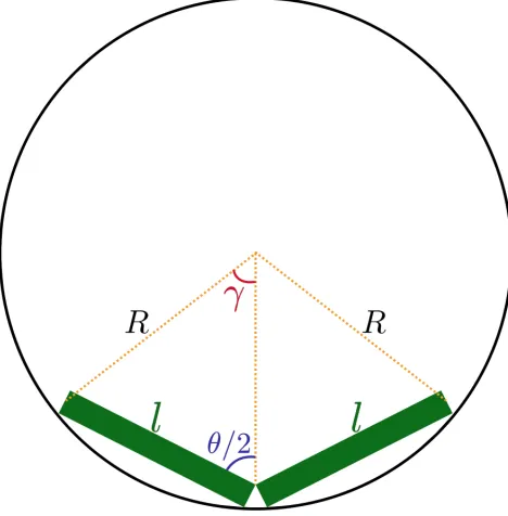
geometry as represented in Figure 2.8:
γ
2π = l
2.3. Flexible Fiber 39
R= l
γ, (2.29)
substituting eq. (2.29) into eq. (2.27)
P =EIAγ
l (2.30)
From the geometry as represented in Figure 2.8:
γ =π−θ (2.31)
and for circular cylinder with diameter d:
IA=
πd4
64 , (2.32)
Substituting eqs. (2.31) and (2.32) into eq. (2.30)
Pb =
πEd4(π−θ)
64l (2.33)
By comparing eq. (2.33) with eq. (2.26):
kb =
πEd4
64l (2.34)
Schmid et. al. [79] and Yamamoto and Matsuoka [65] obtained the same expression
for kb. As seen from Figure 2.8, one of the base assumptions of this calculation is
that the length of the arc with radius of curvature R is equal to 2l, which is correct for small deformations. As the deformation of the fiber increases the model will


![Figure 3.4: Comparison between simulation and experimental [34] periods of rotation ofa rigid fiber as a function of aspect ratio.](https://thumb-us.123doks.com/thumbv2/123dok_us/7732170.1265931/65.612.80.513.474.677/figure-comparison-simulation-experimental-periods-rotation-ber-function.webp)