SPEECH ENHANCEMENT USING AN ADAPTIVE WIENER FILTERING APPROACH
M. A. Abd El-Fattah, M. I. Dessouky, S. M. Diab and F. E. Abd El-samie
Department of Electronics and Electrical communications Faculty of Electronic Engineering
Menoufia University Menouf, Egypt
Abstract—This paper proposes the application of the Wiener filter in
an adaptive manner in speech enhancement. The proposed adaptive Wiener filter depends on the adaptation of the filter transfer function from sample to sample based on the speech signal statistics (mean and variance). The adaptive Wiener filter is implemented in time domain rather than in frequency domain to accommodate for the varying nature of the speech signal. The proposed method is compared to the traditional Wiener filter and the spectral subtraction methods and the results reveal its superiority.
1. INTRODUCTION
Speech enhancement is one of the most important topics in speech signal processing. Several techniques have been proposed for this purpose like the spectral subtraction approach, the signal subspace approach, adaptive noise canceling and the iterative Wiener filter [1– 5]. The performances of these techniques depend on the quality and intelligibility of the processed speech signal. The improvement in the speech signal-to-noise ratio (SNR) is the target of most techniques.
Spectral subtraction is the earliest method for enhancing speech degraded by additive noise [1]. This technique estimates the spectrum of the clean (noise-free) signal by the subtraction of the estimated noise magnitude spectrum from the noisy signal magnitude spectrum while keeping the phase spectrum of the noisy signal. The drawback of this technique is the residual noise.
colored noise [6, 7]. The idea of this algorithm is based on the fact that the vector space of the noisy signal can be decomposed into a signal plus noise subspace and an orthogonal noise subspace. Processing is performed on the vectors in the signal plus noise subspace only, while the noise subspace is removed first. Decomposition of the vector space of the noisy signal is performed by applying the singular value decomposition or the Karhunen-Loeve transform (KLT) on the speech signal[8]. Mi et al. have proposed the signal/noise KLT based approach for the removal of colored noise [9]. The idea of this approach is that noisy speech frames are classified into speech-dominated frames and noise-dominated frames. In the speech-dominated frames, the signal KLT matrix is used and in the noise-dominated frames, the noise KLT matrix is used.
In this paper, we present a new technique to improve the SNR in the enhanced speech signal by using an adaptive implementation of the Wiener filter. This implementation is performed in the time domain to accommodate for the varying nature of the signal.
The paper is organized as follows. In Section 2, a review of the spectral subtraction technique is presented. In Section 3, the traditional Wiener filter in frequency domain is revisited. Section 4 proposes the adaptive Wiener filter approach for speech enhancement. In Section 5, a comparative study between the proposed adaptive Wiener filter, the Wiener filter in frequency domain and the spectral subtraction approach is presented.
2. SPECTRAL SUBTRACTION
The spectral subtraction approach can be categorized as a non-parametric approach, which simply needs an estimate of the noise spectrum. It is assumed that there is an estimate of the noise spectrum which is obtained during periods of speaker silence. Letx(n) be a noisy speech signal:
spectrum as follows [10]:
ˆ
S(ω) = (|X(ω)| −Nˆ(ω)) exp(j∠X(ω)) (2) The estimated time-domain speech signal is obtained as the inverse Fourier transform of ˆS(ω).
Another way to recover the clean signals(n) from the noisy signal
x(n) using the spectral subtraction approach is performed by assuming that there is an estimate of the power spectrum of the noise Pv(ω), which is obtained by averaging over multiple frames of a known noise segment. An estimate of the short-time squared magnitude spectrum of the clean signal using this method can be obtained as follows [8]:
Sˆ(ω)2 =
|X(ω)|2−Pˆv(ω), if |X(ω)|2−Pˆv(ω)≥0
0, otherwise
(3)
It is possible to combine this magnitude spectrum estimate with the phase of the noisy signal and then get the Short Time Fourier Transform (STFT) estimate of the clean signal as follows::
ˆ
S(ω) =Sˆ(ω)ej∠X(ω) (4) A noise-free signal estimate can then be obtained with the inverse Fourier transform. This noise reduction method is a specific case of the general technique given by Weiss et al. and extended by Berouti et al. [2, 12].
The spectral subtraction approach can be viewed as a filtering operation where high SNR regions of the measured spectrum are attenuated less than low SNR regions. This formulation can be given in terms of the SNR defined as:
SN R= |X(ω)|
2
ˆ
Pv(ω)
(5)
Thus, Eq. (3) can be rewritten as:
Sˆ(ω)2=|X(ω)|2− ˆ
Pv(ω)≈ |X(ω)|2
1 + 1
SN R −1
(6)
3. WIENER FILTER IN FREQUENCY DOMAIN
The Wiener filter is a popular technique that has been used in many signal enhancement methods. The basic principle of the Wiener filter is to obtain an estimate of the clean signal from that corrupted by additive noise. This estimate is obtained by minimizing the Mean Square Error (MSE) between the desired signals(n) and the estimated signal ˆs(n). The frequency domain solution to this optimization problem gives the following filter transfer function [13]:
H(ω) = Ps(ω)
Ps(ω) +Pv(ω)
(7)
wherePs(ω) andPv(ω) are the power spectral densities of the clean and the noise signals, respectively. This formula can be derived considering the signalsand the noisevas uncorrelated and stationary signals. The SNR is defined by [13]:
SN R= Ps(ω) ˆ
Pv(ω)
(8)
This definition can be incorporated to the Wiener filter equation as follows:
H(ω) =
1 + 1
SN R −1
(9)
The drawback of the Wiener filter is the fixed frequency response at all frequencies and the requirement to estimate the power spectral density of the clean signal and noise prior to filtering.
Space-variant h(n)
Measurement of speech local statistics Degraded speech
signal x(n)
Enhanced speech signal s(n)
Figure 1. Adaptive Wiener filtering approach for speech
enhancement.
4. THE PROPOSED ADAPTIVE WIENER FILTER
block diagram of the proposed approach is illustrated in Fig. 1. In this approach, the estimated speech signal mean mx and variance σx2 are exploited.
It is assumed that the additive noisev(n) is of zero mean and has a white nature with variance of σ2v. Thus, the power spectrumPv(ω) can be approximated by:
Pv(ω) =σv2 (10) Consider a small segment of the speech signal, in which the signal
x(n) is assumed to be stationary, The signal x(n) can be modeled by:
x(n) =mx+σxw(n) (11) where mx and σx are the local mean and standard deviation of x(n).
w(n) is a unit variance noise.
Within this small segment of speech, the Wiener filter transfer function can be approximated by:
H(ω) = Ps(ω)
Ps(ω) +Pv(ω) =
σ2 s
σ2 s+σ2v
(12)
From Eq. (12), because H(ω) is constant over this small segment of speech, the impulse response of the Wiener filter can be obtained by:
h(n) = σ
2 s
σ2 s+σ2v
δ(n) (13)
From Eq. (13), the enhanced speech signal ˆs(n) in this local segment can be expressed as:
ˆ
s(n) =mx+ (x(n)−mx)∗ σ 2 s
σ2 s+σ2v
δ(n) =mx+ σ 2 s
σ2 s+σv2
(x(n)−mx) (14)
Ifmx and σs are updated at each sample, we can say: ˆ
s(n) =mx(n) + σ 2 s(n)
σ2
s(n) +σv2
(x(n)−mx(n)) (15) In Eq. (15), the local mean mx(n) and (x(n)−mx(n)) are modified separately from segment to segment and then the results are combined. If σ2
Notice that mx is identical to ms when mv is zero. So, we can estimatemx(n) in Eq. (15) from x(n) b y:
ˆ
ms(n) = ˆmx(n) = 1 (2M+ 1)
n+M
k=n−M
x(k) (16)
where (2M+ 1) is the number of samples in the short segment used in the estimation.
To measure the local statistics of the speech signal, we need to estimate the signal variance σ2s. Since σx2 =σs2+σ2v, then σs2(n) may be estimated fromx(n) as follows:
ˆ
σs2(n) =
ˆ
σ2x(n)−σˆv2, if ˆσx2(n)>σˆ2v 0, otherwise
(17a)
where
ˆ
σx2(n) = 1 (2M+ 1)
n+M
k=n−M
(x(k)−mˆx(n))2 (17b)
-10 -5 0 5 10 15 20 25 30 35
0 10 20 30 40 50 60 70 80
Input SNR (dB)
Output PSNR (dB)
Spectral Subtraction Wiener Filter Adaptive Wiener Filter
Figure 2. PSNR results for white noise case at −10 dB to +35 dB
SNR levels for Handle signal.
-10 -5 0 5 10 15 20 25 30 35 0
10 20 30 40 50 60
Input SNR (dB)
Output PSNR (dB)
Spectral Subtraction Wiener Filter
Adaptive Wiener Filter
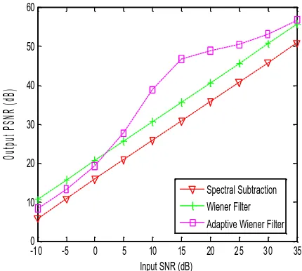
Figure 3. PSNR results for white noise case at −10 dB to +35 dB
SNR levels for Laughter signal.
-10 -5 0 5 10 15 20 25 30 35
0 10 20 30 40 50 60 70 80
Input SNR (dB)
Output PSNR (dB)
Spectral Subtraction Wiener Filter Adaptive Wiener Filter
Figure 4. PSNR results for white noise case at −10 dB to +35 dB
0 0.1 0.2 0.3 0.4 0.5 0.6 0.7 0.8 0.9 1 2000
4000 6000 8000
Time (a)
)
z
H(
y
c
n
e
u
q
er
F
0 1 2 3 4 5 6 7 8
x 104 -1
-0.5 0 0.5 1
Time(msec) (b)
e
d
uti
l
p
m
A
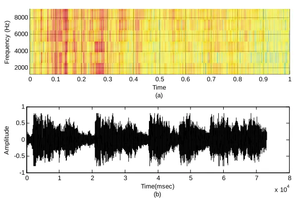
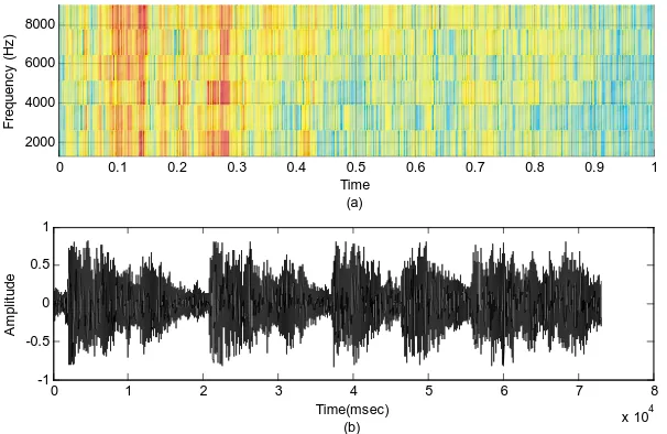
Figure 5. The clean signal. (a) The spectrogram. (b) The time signal.
5. EXPERIMENTAL RESULTS
For evaluation purposes, we use different speech signals; the handle, the laughter and the gong signals. The noisy signal is obtained by adding white gaussian noise to the speech signal with different SNR values. The output peak signal to noise ratio (PSNR) results for the wiener filter, the spectral subtraction approach and the proposed adaptive wiener filter are shown in Figs. 2, 3 and 4. From these figures, it is clear that the proposed adaptive wiener filter has the best performance for different SNR values. The adaptive wiener filter approach gives about 3–5 dB improvement at different values of SNR.
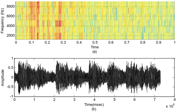
Some experiments are carried out on the handle signal shown in Fig. 5 with SNR values from of 5 to 20 dB to test all the speech enhancement algorithms mentioned in this paper. In all of these experiments, the spectrogram is used with the time signal to clarify the time and frequency contents of the signal. The noisy handle signal with SNR values from 5 to 20 dB in 5 dB steps are shown in Fig. 6.
0 0.1 0.2 0.3 0.4 0.5 0.6 0.7 0.8 0.9 1 2000
4000 6000 8000
Time (a)
)
z
H(
y
c
n
e
u
q
er
F
Figure 6a. The noisy signal at SNR = 5 dB (a) The spectrogram, (b)
The time signal.
0 0.1 0.2 0.3 0.4 0.5 0.6 0.7 0.8 0.9 1
2000 4000 6000 8000
Time (a)
)
z
H(
y
c
n
e
u
q
er
F
0 1 2 3 4 5 6 7 8
x 104 -1
0 1
Time(msec) (b)
e
d
uti
l
p
m
A
Figure 6b. The noisy signal at SNR = 10 dB (a) the spectrogram,
0 0.1 0.2 0.3 0.4 0.5 0.6 0.7 0.8 0.9 1 2000
4000 6000 8000
Time (a)
)
z
H(
y
c
n
e
u
q
er
F
0 1 2 3 4 5 6 7 8
x 104 -1
-0.5 0 0.5 1
Time(msec) (b)
e
d
uti
l
p
m
A
Figure 6c. The noisy signal at SNR = 15 dB (a) The spectrogram,
(b) The time signal.
0 0.1 0.2 0.3 0.4 0.5 0.6 0.7 0.8 0.9 1
2000 4000 6000 8000
Time (a)
)
z
H(
y
c
n
e
u
q
er
F
0 1 2 3 4 5 6 7 8
x 104 -1
-0.5 0 0.5 1
Time(msec) (b)
e
d
uti
l
p
m
A
Figure 6d. The noisy signal at SNR = 20 dB (a) the spectrogram,
0 0.1 0.2 0.3 0.4 0.5 0.6 0.7 0.8 0.9 1 2000
4000 6000 8000
Time (a)
)
z
H(
y
c
n
e
u
q
er
F
0 1 2 3 4 5 6 7 8
x 104 -1
-0.5 0 0.5 1
Time(msec) (b)
e
d
uti
l
p
m
A
Figure 7a. The spectral subtraction technique at SNR = 5 dB (a) the
spectrogram, (b) The time signal.
0 0.1 0.2 0.3 0.4 0.5 0.6 0.7 0.8 0.9 1
2000 4000 6000 8000
Time (a)
)
z
H(
y
c
n
e
u
q
er
F
0 1 2 3 4 5 6 7 8
x 104 -1
-0.5 0 0.5 1
Time(msec) (b)
e
d
uti
l
p
m
A
Figure 7b. The spectral subtraction at SNR = 10 dB (a) The
0 0.1 0.2 0.3 0.4 0.5 0.6 0.7 0.8 0.9 1 2000
4000 6000 8000
Time (a)
)
z
H(
y
c
n
e
u
q
er
F
0 1 2 3 4 5 6 7 8
x 104 -1
-0.5 0 0.5 1
Time(msec) (b)
e
d
uti
l
p
m
A
Figure 7c. The spectral subtraction technique at SNR = 15 dB (a)
The spectrogram, (b) The time signal.
0 0.1 0.2 0.3 0.4 0.5 0.6 0.7 0.8 0.9 1
2000 4000 6000 8000
Time (a)
)
z
H(
y
c
n
e
u
q
er
F
0 1 2 3 4 5 6 7 8
x 104 -1
-0.5 0 0.5 1
Time(msec) (b)
e
d
uti
l
p
m
A
Figure 7d. The spectral subtraction technique at SNR = 20 dB (a)
0 0.1 0.2 0.3 0.4 0.5 0.6 0.7 0.8 0.9 1 2000
4000 6000 8000
Time (a)
)
z
H(
y
c
n
e
u
q
er
F
0 1 2 3 4 5 6 7 8
x 104 -1
-0.5 0 0.5 1
Time(msec) (b)
e
d
uti
l
p
m
A
Figure 8a. The Wiener filter technique At SNR = 5 dB (a) The
spectrogram, (b) The time signal.
0 0.1 0.2 0.3 0.4 0.5 0.6 0.7 0.8 0.9 1
2000 4000 6000 8000
Time (a)
)
z
H(
y
c
n
e
u
q
er
F
0 1 2 3 4 5 6 7 8
x 104 -1
-0.5 0 0.5 1
Time(msec) (b)
e
d
uti
l
p
m
A
Figure 8b. The Wiener filter technique At SNR = 10 dB (a) The
0 0.1 0.2 0.3 0.4 0.5 0.6 0.7 0.8 0.9 1 2000
4000 6000 8000
Time (a)
)
z
H(
y
c
n
e
u
q
er
F
0 1 2 3 4 5 6 7 8
x 104 -1
-0.5 0 0.5 1
Time(msec) (b)
e
d
uti
l
p
m
A
Figure 8c. The Wiener filter technique At SNR = 15 dB (a) The
spectrogram, (b) The time signal.
0 0.1 0.2 0.3 0.4 0.5 0.6 0.7 0.8 0.9 1
2000 4000 6000 8000
Time (a)
)
z
H(
y
c
n
e
u
q
er
F
0 1 2 3 4 5 6 7 8
x 104 -1
-0.5 0 0.5 1
Time(msec) (b)
e
d
uti
l
p
m
A
Figure 8d. The Wiener filter technique At SNR = 20 dB (a) The
0 0.1 0.2 0.3 0.4 0.5 0.6 0.7 0.8 0.9 1 2000
4000 6000 8000
Time (a)
)
z
H(
y
c
n
e
u
q
er
F
0 1 2 3 4 5 6 7 8
x 104 -1
-0.5 0 0.5 1
Time(msec) (b)
e
d
uti
l
p
m
A
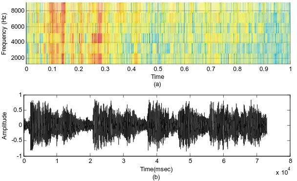
Figure 9a. The adaptive Wiener filter technique At SNR = 5 dB (a)
The spectrogram, (b) The time signal.
0 0.1 0.2 0.3 0.4 0.5 0.6 0.7 0.8 0.9 1
2000 4000 6000 8000
Time (a)
)
z
H(
y
c
n
e
u
q
er
F
0 1 2 3 4 5 6 7 8
x 104 -1
-0.5 0 0.5 1
Time(msec) (b)
e
d
uti
l
p
m
A
Figure 9b. The adaptive Wiener filter technique At SNR = 10 dB (a)
0 0.1 0.2 0.3 0.4 0.5 0.6 0.7 0.8 0.9 1 2000
4000 6000 8000
Time (a)
)
z
H(
y
c
n
e
u
q
er
F
0 1 2 3 4 5 6 7 8
x 104 -1
-0.5 0 0.5 1
Time(msec) (b)
e
d
uti
l
p
m
A
Figure 9c. The adaptive Wiener filter technique At SNR = 15 dB (a)
The spectrogram, (b) The time signal.
0 0.1 0.2 0.3 0.4 0.5 0.6 0.7 0.8 0.9 1
2000 4000 6000 8000
Time (a)
)
z
H(
y
c
n
e
u
q
er
F
0 1 2 3 4 5 6 7 8
x 104 -1
-0.5 0 0.5 1
Time(msec) (b)
e
d
uti
l
p
m
A
Figure 9d. The adaptive Wiener filter technique At SNR = 20 dB (a)
Table 1. PSNR results in dB for the speech enhancement approaches applied to the handle signal at different SNR values.
SNR Noisy Signal Spectral subtraction
Frequency domain Wiener
filter
Adaptive Wiener Filter
5 dB 19.1383 19.1407 22.7568 28.6086 10 dB 24.1217 24.1228 28.9876 32.9784 15 dB 29.1543 29.1547 32.0856 37.3434 20 dB 34.1144 34.1146 37.5216 40.1843
6. CONCLUSION
An adaptive Wiener filter approach for speech enhancement has been proposed in this paper. A mathematical derivation of the filter transfer function has been introduced. This filter is applied by the adaptation of its transfer function from sample to sample based on the speech signal statistics (mean and variance). The experimental results indicate that the proposed filter provides the best PSNR improvement among the spectral subtraction approach and the traditional Wiener filter approach which is implemented in the frequency domain.
REFERENCES
1. Boll, S. F., “Suppression of acoustic noise in speech using spectral subtraction,” IEEE Trans. Acoust., Speech, Signal Processing, Vol. ASSP-27, 113–120, 1979.
2. Berouti, M., R. Schwartz, and J. Makhoul, “Enhancement of speech corrupted by acoustic noise,” Proc. IEEE Int. Conf. Acoust., Speech Signal Processing, 208–211, 1979.
3. Ephriam, Y. and H. L. van Trees, “A signal subspace approach for speech enhancement,” Proc. International Conference on Acoustic, Speech and Signal Processing, Vol. 2, 355–358, Detroit, MI, USA., May 1993.
4. Haykin, S., Adaptive Filter Theory, Prentice-Hall, ISBN 0-13-322760-X, 1996.
5. Lim, J. S. and A. V. Oppenheim, “All-pole modelling of degraded speech,” IEEE Trans. Acoust., Speech, Signal Processing, Vol. ASSP-26, June 1978.
subspace approach for speech enhancement,”IEEE ICASSP, 804– 807, 1995.
7. Hu, Y. and P. Loizou, “A subspace approach for enhancing speech corrupted by colored noise,” Proc. International Conference on Acoustics, Speech and Signal Processing, Vol. 1, 573–576, Orlando, FL, USA, May 2002.
8. Rezayee, A. and S. Gazor, “An adaptive KLT approach for speech enhancement,”IEEE Trans. Speech Audio Processing, Vol. 9, 87– 95, Feb. 2001.
9. Mittal, U. and N. Phamdo, “Signal/noise KLT based approach for enhancing speech degraded by colored noise,”IEEE Trans. Speech Audio Processing, Vol. 8, No. 2, 159–167, 2000.
10. Deller, J. R., J. G. Proakis, and J. H. L. Hansen, Discrete-Time Processing of Speech Signals, Prentice-Hall, 1997.
11. Boll, S. F., “Suppression of acoustic noise in speech using spectral subtraction,”IEEE Trans. Acoustics, Speech, and Signal Processing, Vol. ASSP-29, No. 2, 113–120, April 1979.
12. Weiss, M. R., E. Aschkenasy, and T. W. Parsons, “Processing speech signal to attenuate interference,”Proc. IEEE Symp. Speech Recognition, 292–293, April 1974.