Comparison of Bootstrap-Estimated and Half Sample- Estimated Kolmogorov-Smirnov Test Statistics

(1)

ISSN 2286-4822 www.euacademic.org

Impact Factor: 3.1 (UIF) DRJI Value: 5.9 (B+)

Comparison of Bootstrap-Estimated and Half

Sample- Estimated Kolmogorov-Smirnov Test

Statistics

OMENSALAM A. JAPAR CHITA P. EVARDONE

Professor, Graduate School Mindanao State University Iligan Institute of Technology The Philippines

Abstract:

In testing goodness-of-fit it involves testing the hypothesis that n independent and identically distributed random variables,

X X

₁

,

₂

,...,

X

n, are drawn from a population with a specified continuous distribution function

F x

₀

( , )



. Most of the time, some or all of the components of



are unknown and must be estimated from the sample x-values. Procedures like the bootstrap and half-sample can be used in estimating these parameters. Using the Kolmogorov-Smirnov (KS) test statistics for goodness-of-fit, the bootstrap and half sample- estimated parameters of this test were compared in terms of their efficiency using the Mean-Squared Error (MSE). It was found that the bootstrap procedure is more efficient than the half-sample thereby resulting to a creation of a normality test software using the Bootstrapped KS test statistics.

Key words: goodness-of-fit test, Kolmogorov-Smirnov test, mean-squared error, bootstrap, half-sample, specified distribution function

1 Introduction

In statistics, one often wishes to test if some observations, say

1

,

2

,...,

n

(2)

population with a cumulative distribution function F x( ) with parameter . This is called a “goodness of fit” test. It involves testing the hypothesis that n independent and identically distributed random variables,

X X

₁

,

₂

,...,

X

n are drawn from a population having a continuous distribution function

F x

₀

( , )



with specified parameters. This simple hypothesis has the form

0

: ( , )

0

( , )

H

F x





F x



. (1.1)

In the early 19th_{century, Kolmogorov introduced a}

“distribution-free” statistic, based on the empirical process, defined as:



0



( )

( ) ,

n

x

n F x

n

F x







x



R. (1.2)

A goodness-of-fit test statistics that is a function of the empirical process



_n

( )

x

is the Kolmogorov-Smirnov (KS) statistic

0

sup

( )

n n

x

D

F x

 





, (1.3)

This function of the empirical process under

H

₀ are asymptotically distribution-free [6, 7, 9] and have distributions which are not dependent on the unknown parameter. This is a desirable property of a test statistic.

However, in many practical situations, some or all of the components of  are unknown and thus, the composite hypothesis to be tested takes the form

0

: ( )

(3)

where  is a parametric family of densities. The asymptotic null distribution of the estimated test statistics may depend in a complex way on the unknown parameters and thus, are not distribution-free. This problem of goodness-of-fit tests was presented in the paper of Babu[1], when the parameters were estimated.

To address this problem, nonparametric resampling methods and distribution-free procedures such as the bootstrap method, were proposed by Gombay and Burke[4] to estimate the unknown parameters. It was shown that the asymptotic behavior of the estimated empirical process and its functions are similar to the specified cases for empirical process and its functions respectively, and are therefore distribution-free [6, 7, 9].

This study aims to verify and further compare the investigation on the asymptotic behavior and efficiency of the estimated empirical process and its related functions based on the bootstrap method and half-sample method via simulation and to create a normality test software using the Bootstrapped KS statistics.

2 Preliminaries

2.1 Goodness-of-Fit Test

Let

X X

₁

,

₂

,...,

X

_n be a random sample from a continuous cumulative function F x( ). The empirical distribution function

( )

n

F x

is a function of

X

_i’s that are less than or equal to

x

, i.e.,

( ) 1

1 ( )

i n

n x x

i

F x

I

n

 





,

   

x

(2.1)

(4)

(1) (2)

...

( )n

X



X

 

X

of the random sample

X X

₁

,

₂

,...,

X

_n,

F x

_n

( )

is given as

(1)

( ) ( 1)

( )

0 ( )

1

n k k

n

if

X

x

k

F x

if

X

x

X

n

if

X

x











_

 







,

k



1,...,

n



1

(2.2)

A goodness-of-fit test is a procedure for determining whether a sample of n observations,

X X

₁

,

₂

,...,

X

n, can be considered as a sample from a given specified distribution function

F x

0

( )

, where,

0

( )

x

F x

f y dy







,

   

x

, and (2.3)

( )

f y

is a specified density function.

2.2 Kolmogorov-Smirnov (KS) Statistic

A goodness-of-fit test is a comparison of

F x

_n

( )

defined in (2.2) with

F x

0

( )

. The hypothesis (1.1) is rejected if the difference between

F x

_n

( )

and

F x

₀

( )

is very large.

The Kolmogorov-Smirnov statistic provides a means of testing whether a set of observations are from some completely specified continuous distribution,

F x

₀

( )

. Kolmogorov [8] introduced the statistic

0

sup

( )

( ,

)

n n

x

D

F x



 





, (2.4)

(5)

2 2

2

lim

_n

( 1)

j j z n j

z

d

e

n

   _



_{  }











, (2.5)

for the probability distribution of

D

_n, where





( ) Pr ob

n n

d   D   . (2.6)

2.3 Bootstrap and Half-sample Method

Bootstrap was first introduced and used by Efron in 1979. The bootstrap creates a large number of datasets by sampling with replacement and computes the statistic on each of these datasets.

The half-sample method is done by sampling a size 2 n

without replacement from the random sample X X₁, ₂,...,X_n from a population with distribution function F x( ).

2.4 Maximum Likelihood Estimators

Let

X X

₁

,

₂

,...,

X

_n be an independent and identically distributed random variables from N( , )  distribution. The maximum likelihood estimators (MLE) of the parameters



are given by

2

ˆ ˆ

( ,  ), where

1

1 ˆ

n _i

i

x

X

n





 



(2.7)

and





2

2 1

ˆ

n i i

X

x

n











(2.8)

(6)

The maximum likelihood estimators of the parameters



were derived by Evardone [7] in her paper to be

   

ˆ

( , )

ˆ

and given as

2

ˆ

x

s





(2.9)

and 2

ˆ

s

x





. (2.10)

2.4 Pointwise Mean-Squared Error (MSE)

Let T be the value of the test statistics at the specified case and

t

_i be the value of the test statistics for

i

th method (i=1 for bootstrap and i=2 for half-sample). The pointwise MSE was the measure computed to compare the simulation results. It is computed as

2

1

(

)

ˆ ( )

k i i i

t

T

MSE t

k









(2.11)

where k = no. of partitions of the test statistics.

3 Methodology

The experiment was conducted by investigating four sample sizes

n

= 50, 150, 300 and 500 from the two distributions: the normal distribution with mean



= 1.0 and variance



2_{= 1.0} and gamma distribution with parameter



= 4.0 and



= 2.0, with 1000 replications for each case. Two resampling methods were used in estimating the parameters, namely: bootstrap and half-sample procedures.

(7)

Step 2. Compute for

F x

_n

( , )

 

P x

(



2)

and which formula is defined in (2.2).

Step 3. Compute for



_n

( )

x



n F x



_n

( , )

 

F x

₀

( , )





, at x = 2, where

F x

₀

( , )



is the value of the normal cumulative distribution function (CDF) at x = 2. This x-value is arbitrarily chosen.

Step 4. For each of the observation x in the sample generated, compute for

F x

_n

( , )

 

F x

₀

( , )



where

F x

₀

( , )



is the normal CDF at x. The maximum of the value computed is the KS statistics defined in (2.4).

Step 5. For bootstrap case, generate a bootstrap sample from the random sample obtained in Step 1 and compute from this bootstrap sample the maximum likelihood estimators (MLE) of the parameter which is

   

ˆ

( , )

ˆ ˆ

. Do step 2 to 4 using this new value of the parameter.

Step 6.Do step 5 using the half-sample method instead of the bootstrap. This is the half-sample case.

All these enumerated steps are repeated 1000 times thus generating 1000 values of



_n

( )

x

and

D

_n for the specified case, bootstrap case and half-sample case for different sample sizes of

n: 50, 150, 300 and 500.

Same procedures were adopted under another

distribution Gam(4, 2). The graphs of the sampling distribution

of these statistics were created at different sample sizes and

two distributions. The whole simulation procedure is shown in

(8)

Fig.3.1 Simulation Diagram

4 Results and Discussion

(9)

4.1 Bootstrap Estimated Empirical Process



_n

( )

x

Legend: Blue (specified case); Red (Bootstrap Case)

Fig.4.1 Cumulative Distribution of the Bootstrap-Estimated



_n

( )

x

against Specified



n

( )

x

from Normal Distribution at Various n

(10)

Fig.4.2 Cumulative Distribution of the Bootstrap-Estimated



_n

( )

x



n

( )

x

from Gamma Distribution at Various n

Fig.4.2 showed that the cumulative distribution of the empirical process of the specified case and the bootstrap case for Gamma distribution is not that close for any values of n as that of the normal distribution.

(11)

Fig.4.3 Cumulative Distribution of the Bootstrap-Estimated KS Statistics against Specified KS Statistics from Normal Distribution at Various n

Fig.4.4 Cumulative Distribution of the Bootstrap-Estimated KS Statistics against Specified KS Statistics from Gamma Distribution at Various n

(12)

Table 4.1 MSE for Bootstrap-Estimated Empirical Process



_n

( )

x

and Kolmogorov-Smirnov Statistics

Sample Size

( )

n

x



KS

Normal Gamma Normal Gamma

50 0.00109 0.00419 0.00031 0.00046

150 0.00067 0.00386 0.00028 0.00005

300 0.00162 0.00172 0.00010 0.00011

500 0.00011 0.00262 0.00028 0.00004

In this paper, the MSE was used as a measure of closeness of the distributions of the bootstrap-estimated statistics and the specified one. As shown in Table 4.1 the MSE of the empirical process



n

( )

x

are close to zero value for the two distributions, normal and gamma. The same was observed for the function of the empirical process which is the KS or

D

_n statistics. The results in the previous graphs were confirmed in this MSE measures. It is confirmed that the sampling distributions of the bootstrap-estimated empirical process and its function are the same with that of the specified case.

(13)

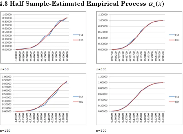
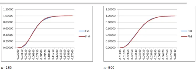
Fig.4.5 Cumulative Distribution of the Half Sample-Estimated



n

( )

x



_n

( )

x

from Normal Distribution at Various n

The result in Fig.4.5 showed that the cumulative distribution of the empirical process of the specified case and the half-sample case is closest already for n = 300.

Fig.4.6 Cumulative Distribution of the Half Sample-Estimated



_n

( )

x



_n

( )

x

from Gamma Distribution at Various n

(14)

4.4 Half Sample-Estimated Kolmogorov-Smirnov Statistics

(15)

Fig.4.8 Cumulative Distribution of the Half Sampled-Estimated KS Statistics against Specified KS Statistics from Gamma Distribution at Various n

Graphically, as shown in Fig.4.7 and Fig.4.8 both for normal and gamma distribution, the cumulative distribution of the half sample-estimated and specified-case KS statistics are very close to each other.

Table 4.2 MSE for Half Sample-Estimated Empirical Process



_n

( )

x

and Kolmogorov-Smirnov Statistics

Sample Size

( )

n

x



KS

Normal Gamma Normal Gamma

50 0.00075 0.00434 0.00080 0.00057

150 0.00087 0.00404 0.00039 0.00014

300 0.00036 0.00091 0.00105 0.00003

500 0.00013 0.00222 0.00023 0.00006

As shown in Table 4.2 the MSE of the empirical process

( )

n

x

(16)

4.5 Bootstrap Kolmogorov-Smirnov Test for Normality Software

Fig.4.9 Bootstrap Kolmogorov-Smirnov Test for Normality Program

A Bootstrap Kolmogorov-Smirnov Test for Normality program was created that test if a sample of size n is coming from a normal distribution. The sample size of the input data for this program is limited to specific sample sizes of 50, 100, 150, or 200. This software makes use of the bootstrap estimated KS to test the hypothesis that the distribution of the data is normal. This program can be open and run using any internet browser.

5 Conclusion

(17)

Using the MSE in comparing the bootstrap and half-sample procedure in terms of their efficiency, it was found that the bootstrap procedure is more efficient than the half-sample method. The bootstrap procedure is good in estimating parameters of the hypothesized continuous distribution since it approximates the sampling distribution of the specified case. It is recommended for future studies that the sample size and the number of iterations in the simulation be increased and to improve the program for any sample size n, and to use R, a free software.

REFERENCES

[1] Babu, Gutti Jogesh. Model fitting in the presence of

nuisance parameters. In Astronomical

Data Analysis-III (2004). Fionn D. Murtagh (Ed.). Electronic Workshops in Computing (EWiC).

[2] Babu, G. J. and C. R. Rao (2003). Goodness-of-fit tests when parameters are estimated. Sankya, 66, 1-12.

[3] Burke, M. D., M. Csorgo, S. Csorgo and P. Revesz (1978). Approximations of the Empirical Process When the Parameters are Estimated. The Annals of Probability. 5, pp. 790-810.

[4] Burke, M. D. and Gombay, E. (1988). On goodness-of-fit and the bootstrap. Statistics and Probability Letters, 6, 287-293. [5] Durbin, J. (1973). Weak Convergence of the sample distribution function when parameters are estimated. Ann. Statist. 1, 279-290.

(18)

[8] Khmaladze, E. V. Goodness-of-fit Problem and Scanning Innovation Martingales. The Annals of Statistics, Vol. 21, No. 2, (1993), 798-829.