Automatic Detection of Eye Blinking Using the Generalized Ising Model

Western University Western University

Scholarship@Western

Scholarship@Western

Electronic Thesis and Dissertation Repository

10-4-2016 12:00 AM

Automatic Detection of Eye Blinking Using the Generalized Ising

Automatic Detection of Eye Blinking Using the Generalized Ising

Model

Model

Marwa Elsayh Dawaga

The University of Western Ontario Supervisor

Andrea Soddu

The University of Western Ontario Graduate Program in Physics

A thesis submitted in partial fulfillment of the requirements for the degree in Master of Science © Marwa Elsayh Dawaga 2016

Follow this and additional works at: https://ir.lib.uwo.ca/etd

Recommended Citation Recommended Citation

Dawaga, Marwa Elsayh, "Automatic Detection of Eye Blinking Using the Generalized Ising Model" (2016). Electronic Thesis and Dissertation Repository. 4351.

Abstract

Electroencephalogram (EEG) is a widely used technique to record electrical brain activity. It is prone to be contaminated by non-neuronal sources that can generate artifacts in the signal due to its sensitivity and its poor signal-to-noise ratio. One of the main challenges in analyzing EEG data is the systematical and effective removal of artifacts from the signal. Although many methods have already been introduced to approach this issue, there is still no robust method for handling all sources of contaminations. For example, eye blinking is a physiological artifact occurring very frequently in spontaneous EEG recordings and therefore, removing these artifacts in a systematic way is a compelling need. The aim of this research is to build an automated pipeline to detect eye blinking artifacts in EEG signals using the generalized Ising model to act as a pattern recognition algorithm. A sample blink pattern is extracted from a single subject whose blink events are validated and marked by an EEG expert. The generalized Ising Model Algorithm works as a fully automated method for identifying all epochs similar to the eye blink pattern. Using the proposed method to discriminate the blinks artifact in continuous EEG data yields optimistic results. From eight healthy subjects, the results show high level of accuracy (90 %).

Dedications

To my wonderful parents, For their support and patience…..

Acknowledgments

The time I spent working on this thesis has been full of incredible moments of learning both on the academic and personal levels. As I am writing those words today, I would like to reflect upon those who were with me through this journey and offered me their help and support.

Firstly, I would like to thank my supervisor Dr. Andrea Soddu for his continuous confidence in me and for providing advice and guidance on every level throughout my Master’s program.

I would also like to express my gratitude to Dr. Tushar K. Das (University of Western Ontario), Dr. Robert Camely (University of Colarado) and Dr. Andrea Piarulli (Scuola Superiore

Sant’Anna) for their invaluable feedback on my work.

Many thanks to my group members for their encouragement and for many insightful discussions. I am particularly grateful to Pubuditha M. Abeyasinghe for her unlimited

support throughout the past two years.

Contents

Abstract ... ……….i

Dedications ... ii

Acknowledgments ... iii

Contents ... .iv

List of Figures ... vii

List of Tables………ix

List of Appendices………x

Chapter 1: Introduction 1.1.Introduction ... …1

1.1.1 History ... ….1

1.1.2 Advantages and Limitations………...2

1.1.3 EEG and ERP………....2

1.2 The Source of EEG Signals……….3

1.3 EEG Recordings………...4

1.4.3 Alpha Waves………...8

1.4.4 Beta Waves………9

1.4.5 Gamma Waves………...9

1.5 EEG Applications………...10

1.6 EEG Artifacts………...10

1.6.1 Muscle Artifacts………..12

1.6.2 Electrocardiogram (ECG)………....12

1.6.3 Ocular Artifacts………....12

1.6.3.1 Eye Movement Artifacts………..13

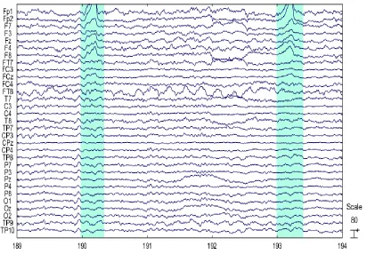
1.6.3.2 Eye Blinking Artifact………..….13

1.7 EEGLAB………...14

1.8 Ising Model………...……….15

Chapter 2: Methodology 2.1 Ising Model………..18

2.2 Monte Carlo Simulation………...21

2.3 Blink Detection in EEG Data………22

2.3.3 EEG Data Simulation………..22

Chapter 3: Results…...……….28

Chapter 4: Discussion and Conclusions……….………..35

4.1 Future Directions………...38

Bibliography………39

Appendices………44

1. Appendix A: Generalized Ising Model Algorithm………...45

2. Appendix B: 2D Channel Locations………....50

3. Appendix C: Gender, Age, and Types of EEG Data of the Subjects Used in This Research………...51

4. Appendix D: Blink Topography……….52

5. Appendix E: Independent Component Analysis Topographies……..53

List of Figures

1.1 The parts of a single pyramidal neuron that connected to three neurons by different types of

synapses………...3

1.2 The lobes of the brain. ………...………….6

1.3 The positions of the electrodes based on the international 10/20 system………...6

1.4 Delta brain wave………...………7

1.5 Theta brain waves.………...………...8

1.6 Alpha brain wave………..….8

1.7 Beta brain wave.………..…...9

1.8 Gamma brain wave.………...9

1.9 Representation of EEG data with different types of artifacts..………...11

1.10 Eye blinking artifacts represented by the highlighted areas in 190 and 193 seconds………..………...14

1.11 Illustration of 2D Ising Model spins. The “red” spin with its four “black” nearest neighbors.………..…...16

2.1. Spin configuration of letter “A” represented by upward spins and with the rest of the spins downward……….………….19

2.2. The representation of “À”, a spin configuration similar to the letter “A”, which can be obtained by perturbing the letter” A”…………...21

2.4. A blink from one channel with chosen baseline……….……25 2.5. Illustration of the shifting by 10 time points showing how a blink from one channel is appearing gradually.……….. ……….. .27 3.1. Representations of the letter “A” in (a) and the similar configuration “À” in (b). If we start with (a), we will eventually have the pattern in (b)………...28 3.2. Representation of a blink in (a) from the second subject which converged to the blink pattern in (b) using the generalized Ising Model………...………29 3.3. Percentage of evolved blinks versus temperature.………....30 3.4. Energy, specific heat, magnetization, and susceptibility vs temperature with critical temperature value………...……...31 3.5 (a). EEG recording for 31 channels with three blinks detected at the time 260,

List of Tables

Table 3.1. Duration of EEG recording in minutes, number of blinks, blink frequency, percentage of TP, TN, FP, FN, sensitivity, specificity and accuracy for six subjects, together with the mean and standard deviation over the six

List of Appendices

Appendix A. The Generalized Ising Model Algorithm……….45 Appendix B. 2D Channel Locations ………...………..………...50 Appendix C. Table 2. Gender, Age, and Types of EEG data of the Subjects That

Chapter 1

Introduction

This thesis consists of four chapters. The first chapter provides details about EEG such as the history, recording techniques, applications etc. followed by a brief introduction of EEGLAB and of the Ising Model. The second chapter includes the methodology of implementing our simulations and modifications that allow the simulation to be applied on EEG data. The third chapter presents the results of the analysis. Finally, in the fourth chapter the discussion and the conclusions are presented.

1.1 Introduction

1.1.1 History

Electroencephalogram (EEG) is a widely used technique to record the oscillations of brain electric potential by placing a set of electrodes over the scalp. The first discovery of the electric activity in rabbits’ and monkeys’ brains, particularly, in cerebral hemispheres was made by the physician Richard Caton in 1875. Subsequently, the neurologist Hans Berger was able to amplify very weak currents recorded from a human scalp, and the name of Electroencephalogram was provided by him. A few years later, the physiciansEdgar Adrian and B.H.C.

1.1.2 Advantages and Limitations

Besides EEG’s extensive use among modern medical tools and burgeoning vital role in both clinical diagnosis and cognitive science, it has also brought significant advantages in comparison to other medical techniques.

In general, EEG is relatively inexpensive if we compare it, for instance, to fMRI (functional Magnetic Resonance Imaging). It is also portable, so it is convenient for those who need it. During an fMRI acquisition applied gradients create a very noisy environment inside the machine, which can be uncomfortable for patients and less beneficial for audio studies. On the other hand, EEG is more convenient for audio studies that require silence. Furthermore, EEG is considered as an accessible method for patients who have motor difficulties. Another advantage of the EEG with respect to fMRI is its higher temporal resolution (~1ms), that allows a continuous recording of even short lasting brain activities.

Nonetheless, EEG also has limitations. Spatial resolution of EEG is relatively poor, which makes it difficult to decide which brain portion actually contributed to the EEG signals. Moreover, EEG is hypersensitive to any electric activity and that can result in detection of other undesirable electric activities [2].

1.1.3 EEG and ERP

temporal resolution of EEG, we can understand more about how different information isprocessed following different stimuli or performing a particular task, and this is considered an extremely strategic aspect for building cognitive neurophysiological tests[3].

1.2 The Source of EEG Signals

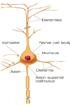
The cerebral cortex of the human brain, which is the folded area, has a thickness between 2-5 mm and contains 105 neurons per 𝑚𝑚2. A neuron essentially consists of a body cell (soma), an axon and dendrites (Figure 1.1).

Figure 1.1. The parts of a single pyramidal neuron that connected to three neurons by different types of synapses [4].

neuron and influence it to fire the action potential. On the other hand, inhibitory postsynaptic potentials (IPSPs) are also generated by a synaptic input and cause the generation of current sources. During the synaptic action, micro currents (𝑁𝑎+, 𝐾+, 𝐶𝑙−) [6] flow into the target neuron membrane. Due to the relatively long distance between the electrodes and the small currents, the principle of dipole approximation can be applied so that the recorded electric signals are considered as the result of electric dipoles activity. Additionally, only a large number of active pyramidal cells can contribute to recorded EEG signals [5].

1.3 EEG Recordings

In order to record EEG signals, a collection of electrodes needs to be placed over the scalp at specific locations. Systems such as 10/20, 10/10 and 10/5 are international criterions used for positioning the electrodes over the scalp [7]. We provide the following explanations about 10/20 because it is simple and give an idea of the electrodes names based on their location. The 10/20 system is the international criteria used to determine the locations of the electrodes. The numbers “10” and “20” refer to the proportional distances between the electrodes based on the total area of the skull which is determined by the anatomical landmarks “nasion”, which is the part of skull between the nose and the “inion” which is the last prominent part of the skull (from front to back), and “ear-lobes” (from right to left) [8].

between 16 and 256. Therefore, any additional electrodes can be placed between the labeled 10/20 system electrodes [8]

Figure 1.2. The lobes of the brain [9].

1.4

EEG Waveforms

The main concern for the cognitive researchers is to link the scalp electric potentials to physiological processes. Therefore, these potentials can be defined based on their temporal and spatial attributes [5]. Specific brain waves can be simply recognized by visual inspection of the EEG signals. These rhythms are also used as signatures of particular diseases or neurological brain states such as dementia and sleep states. [11]. In essence, five main brain rhythms are identified by specific frequency ranges and named based on the Greek alphabet, Delta, Theta, Alpha, Beta, and Gamma.

1.4.1 Delta Waves

In human EEG recordings, delta waves are the waves with the lowest frequencies at < 4 Hz. They appear frequently in recordings of infants, of people with brain injuries and with learning difficulties [12], but most importantly during deep sleep in healthy subjects [13].

Figure 1.4. Delta brain wave [14].

0 0.5 1 1.5 2 2.5 3 3.5 4 4.5 5

5 0

-5

1.4.2 Theta Waves

Theta waves’ frequency lies between 4-8 Hz. They are mainly produced from the frontal region of the brain. In addition, these signals can be associated with sleep disorder and brain tasks that require concentration [15].

Figure 1.5. Theta waves [14].

1.4.3 Alpha Waves

Alpha was the first discovered and recorded brain oscillation. This waveform can be found in a recording of healthy adults in a state of relaxation and with closed eyes. The frequency ranges between 8 and 12 Hz, and the largest amplitude of Alpha waves can be recorded from the parietal and occipital brain lobes [15].

Figure 1.6. Alpha brain wave [14].

0 0.5 1 1.5 2 2.5 3 3.5 4 4.5 5

5 0

-5

Time (s)

0 0.5 1 1.5 2 2.5 3 3.5 4 4.5 5

5 0

-5

1.4.4 Beta Waves

The frequency of beta wave lies between 12 and 30 Hz. It is mostly recorded from the frontal and central areas of the brain and related to concentration and brain tasks. The high level of beta occurs as a result of a participant’s stress as well [13].

Figure 1.7. Beta brain wave [14].

1.4.5 Gamma Waves

These waves are distinguished from their considered relatively high frequency, 30 Hz and above. Gamma waveform is related to attention. For example, they appear during the sensing of certain stimuli [16].

Figure 1.8. Gamma brain wave [14].

0 0.5 1 1.5 2 2.5 3 3.5 4 4.5 5

5 0

-5

Time (s)

0 0.5 1 1.5 2 2.5 3 3.5 4 4.5 5

5 0

-5

1.5

EEG Applications

Some people recognise the EEG cap through its use with epilepsy. Epilepsy is a brain disorder that can be caused by brain injury, illness, or developmental problems though there are also many cases where the causes are still unidentified [17] and consists of an over-excitability of the involved cortex.

EEG plays an important role in diagnosing and monitoring epilepsy seizures. It is considered the gold standard for diagnosing epilepsy, and has achieved continuous medical development to help patients who experience that disorder [18]. In addition, EEG is used in diagnosing sleep disorders, dementia, brain tumours and brain death. Moreover, EEG is used extensively in cognitive science research, for instance, in those processes that are related to memory, attention, language and emotions because it is a non-invasive technique [1].

1.6 EEG Artifacts

Figure 1.9. Representation of EEG data with different types of artifacts.

1.6.1 Muscle Artifacts

Although the time range for muscle activities is short, it is still important to determine which signals refer to the muscle activity as their frequency range is wide (10 < 500 Hz). The board frequency range implies that the muscle artifacts can be easily correlated with EEG frequency bands. These artifacts also known as electromyogram (EMG) contaminations. To ensure successful recognition and removal for EMG from the EEG recordings, it is better to understand deeply their spectral distribution rather than their frequency [21]. This type of noise can be controlled by the restriction of the subjects’ motor activity during the spontaneous EEG recording. However, it is still challenging to eliminate these artifacts in sleep recordings that are mostly contaminated (20-70 % of the all-night recording) [22].

1.6.2

Electrocardiogram

(ECG)

These signal are generated by the heart beating potential and often overlap with the EEG signals, especially in subjects with short necks. ECG is a type of signal that can be simply recognized in the EEG recording because it is characterized based on its shape, which appears like a spike, its repetitive occurrence and its lack of correlation with EEG signal. [20]. Due to its relative stationarity, the ECG artefact can be effectively removed using methods such as independent component analysis [23].

result of changes in the electric potential of the eye and the way this electric change is produced depends on the type of eye artifact [24]. In essence, there are two main ocular artifacts, which are the eye movement and the eye blinking.

1.6.3.1 Eye Movement Artifacts

The movement of the eyeball is responsible for these artifacts, and that essentially results in the retino-corneal dipole where the cornea is positively charged with respect to the retina [25]. Based on the direction of the eyeball’s movement, we can determine which electrodes are going to be more affected than the others. For instance, if the eyeball is moving vertically, the electrodes such as Fp1 and Fp2 are going to have agreater influence as they are located closely above the eye. On the other hand, the greatest electric potential change will occur to the electrodes F7, in the case of horizontal eyeball movement. [24].

1.6.3.2 Eye Blinking Artifacts

Figure 1.10. Eye blinking artifacts represented by the highlighted areas in 190 and 193 seconds.

1.7

EEGLAB

1.8

Ising Model

In early 1920s, Wilhelm Lenz studied the phase transition of ferromagnetism in 1-dimintional (chain) spin systems, and that was suggested to be his PhD students’ (Ising) proposal [28]. The ferromagnetic materials are known by their spontaneous magnetization due to the alignment of the spins (magnetic moments) in the same direction. Once the temperature of these materials starts increasing, a critical temperature is reached when there is a sudden change of the spins direction. This phenomenon known as phase transition [29].

Ising’s first results were not as he expected, and he concluded that there is no phase transition in 1D (1-dimensional) nor in higher dimensions (D > 1) spin systems [30]. However, eventually, scientists proved that there is actually a phase transition in 2D systems.

In 1952, Onsager obtained the exact solution for 2D Ising model. Although it is considered to be a simple model, the use of this model has recently increased in many scientific applications [28] as it is straightforward to solve both 1D and 2D Ising models [31].

The total Energy of state can be described by Equation (1.1) in the absence of an external magnetic field.

𝐸 = −𝐽 ∑

𝑆

𝑆

(1.1)

Where E is the total energy, J is the coupling constant, 𝑆_𝑖 and 𝑆_𝑗 are the spins in the sites i

In this Model, the interactions occur between the spins and its nearest neighbors. Figure 1.11 shows

a 2D Ising Model as an example. The number of nearest neighbors for a lattice of size N depends

on the systems’ dimensionality which can be obtained using 2𝑑 where d is the dimensionality.

Figure 1.11. Illustration of 2D Ising Model spins. The “red” spin with its four “black” nearest

neighbors.

Since we consider the Ising Model as a system in equilibrium with a “heat bath”, that implies that we study the system in each equilibrium state (with a fixed temperature T). At the temperature T a configuration “c” is acquired with a probability:

𝑝 =

𝑍

𝑒

−𝐸𝑐

𝐾𝐵𝑇

(1.2)

𝑍 = ∑ 𝑒

−𝐸𝑐 𝐾𝐵𝑇

where Z is the partition function, 𝐸𝑐 is the energy and 𝐾𝐵 is the Boltzmann constant [32] and the

sum in the partition function definition is extended to all possible configurations. Because of the

large number of possible configurations (2𝑁_{for N lattice sites),it is better to be solved numerically}

using the Monte Carlo simulations (See Chapter 2).

For the Ising Model, two more representative configurations of spins can be obtained. One, the low energy state or ground state, occurs when the temperature is zero and the spins are aligned in the same direction with an average magnetization of one. The second one can be found at a much higher temperature in which the spins can be directed in one of the two possible direction and the average magnetization is zero. These spin configurations correspond to two distinct phases, which are ferromagnetic and paramagnetic in the case of classical Ising Model. In addition, the state shift can occur related to the temperature of the system: the critical temperature 𝑇𝑐 correspond to the

Chapter 2

Methodology

2.1 Ising Model

The Ising Model is a model that studies the physics of phase transition in ferromagnetism. In 1925, it was introduced by Ernst Ising as his PhD dissertation. The model describes a system that consists of spins (magnetic moments) in a lattice and each spin interacts only with its nearest neighbors

with equal couplings across the lattice [34].

Since the model has been used in many scientific applications and can be handled numerically, its

actual description for phase transition from ferromagnetic to paramagnetic is called the classical

Ising model. Its generalization with non-uniform couplings is usually called the generalized Ising

model.

The total energy of the classical Ising model is defined by the following equation:

𝐸 = −𝐽 ∑_<𝑖,𝑗>𝑆_𝑖 𝑆_𝑗 − ℎ ∑ 𝑆_{𝑖 𝑖} (2.1)

where J is the coupling constant, the notation< 𝑖, 𝑗 > refers to the summation over the nearest

the spins take either the value +1 for the upward direction or -1 for the downward direction; therefore, from Equation (2.2) we can deduce that as the spins are aligned in the same direction (ordered spins), the energy will have the lowest energy value.

In this research, we are considering the generalized Ising model where the J (coupling constant) is going to be different from the classical coupling, and the choice of 𝐽𝑖𝑗 is set in order to use the

generalized Ising model as a pattern recognition tool.

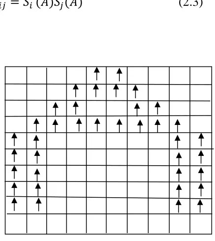
Let’s assume for a 10x10 square lattice, the 𝐽_𝑖𝑗 can be defined as in Equation (2.3) for a well-defined configuration as, for instance, in the letter “A” case (see Figure 2.1). As shown in Figure 2.1 the upward spins are visible, while the downward spins are represented by blank sites.

𝐽_𝑖𝑗 = 𝑆_𝑖 (𝐴)𝑆_𝑗(𝐴) (2.3)

.

Based on the assumption that 𝐽_𝑖𝑗 = 𝑆_𝑖 (𝐴)𝑆_𝑗(𝐴), we can calculate the energy as:

𝐸 = − ∑ 𝐽_{𝑖,𝑗 𝑖𝑗} 𝑆_𝑖 𝑆_𝑗 (2.4)

which for the particular ‘A’ spin configuration gives

𝐸 = − ∑ (𝑆_{𝑖,𝑗 𝑖} (𝐴)𝑆_𝑗 (𝐴))(𝑆_𝑖(𝐴)𝑆_𝑗(𝐴)) (2.5)

Since the 𝑆_𝑖 and 𝑆_𝑗 can be either +1 or -1, and both i and j go from 1 to the number of lattice sites (N), then :

𝐸 = −𝑁2. (2.6)

an initial configuration to a more favourable one by randomly flipping spins in a Monte Carlo simulation (explained in Section 2.2).

Figure 2.2. The representation of “À”, a spin configuration similar to the letter “A”, which can be obtained by perturbing the letter “A”.

2.2 Monte Carlo Simulation

Monte Carlo methods are computational techniques commonly used in scientific applications in order to obtain a valid approximation of the solution of the problem in a reasonable computational timing. This technique allows for the estimation of the statistical properties of the Ising model by generating the more likely configurations of the system [35].

Considering the configuration in Figure 2.2 as the starting configuration, we can describe the Monte Carlo simulation in the following steps:

1. Choose a spin randomly to flip.

3. Check the condition ∆𝐸 < 0, and if the condition is satisfied then accept the flip.

4. If ∆𝐸 > 0, then accept the flip with probability p=exp (−∆𝐸/𝐾𝑇) ; otherwise, reject the flip and return to the original configuration.

5. Finally, to obtain the equilibrium energy, repeat the previous steps for a number of required trials.

2.3 Blink Detection in EEG Data

2.3.1 Subjects

EEG data acquired from eight healthy subjects, with mean age 46± 15, including three females. (Appendix C).

2.3.2 EEG Data Acquisition

For EEG data acquisition, the system that composed of 256 is used to record EEG data ( For the purposes of our research, only 32 channels have been selected and the recordings obtained by using 250 Hz as a sampling rate.

2.3.3 EEG Data Simulation

In the previous section, we discussed the potential convergence of an initial configuration to a chosen pattern.

As we explained previously, the spontaneous EEG data have been obtained from eight healthy subjects (mean age 46± 15, 3 females) by selecting 32 electrodes from a 256 net where the Cz is used as the reference electrode. From the eight subjects, the first two subjects’ continuous recording EEG were used to extract blink events (extraction was made by an EEG expert). The blink events extracted from the first subject were employed to build an average blink pattern, while the blink events extracted from the second subject were used as the initial configurations. Then their convergence to the average blink pattern was tested.

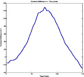
Figure 2.3. Average blink time profile when looking at the first channel.

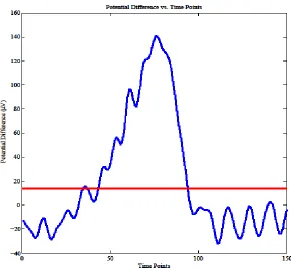
Figure 2.4. A blink from one channel with chosen baseline.

The same baseline for all the 12 channels has been adopted and a value of +1 and -1 have been assigned for a signal respectively greater and lower than the baseline producing a 12x30 blink pattern of ±1.

Using exactly the same procedure as for the letter A, the average blink pattern configuration has been subsequently adopted to build the couplings 𝐽𝑖𝑗(𝐵𝑙𝑖𝑛𝑘) = 𝑆𝑖 (𝐵𝑙𝑖𝑛𝑘)𝑆𝑗(𝐵𝑙𝑖𝑛𝑘) with the

happened, full overlap or zero distance between the two configurations, we could claim that the blink was recognized by our detector.

Chapter 3

Results

The simulation of the generalized Ising model as a pattern recognition has been performed using a home made MATLAB program developed by a previous code by Tushar Das. Our initial investigation consisted in testing the convergence of a marginally altered two dimensional pattern to the original pattern. We then created a letter “A” using a 10x10 matrix based on the up spins, and subsequently the corresponding 𝐽_𝑖𝑗. As we discussed in the methods, another configuration similar to the letter “A” has been also built by mildly perturbing the configuration “A”, and we called it “À”. What we showed that if we use “À” as an initial configuration, the generalized Ising Model Algorithm will converge to the letter “A” pattern (Figure 3.1).

Similarly, for the 12x30 blink pattern, its 𝐽_𝑖𝑗 has been built, and the 84 blinks extracted from the second subject were used as an initial configurations and tested for convergence to the average blink obtained from the very first subject. We found that all the blinks evolved to the blink pattern. See Figure 3.2 (a) for an example of a blink out of the 84 extracted from the second subject, and Figure 3.2 (b) for the average blink pattern from the very first subject respectively.

Figure 3.2. Representation of a blink in (a) from the second subject which converged to the blink pattern in (b) using the generalized Ising Model.

Figure 3.3. Percentage of evolved blinks versus temperature.

Figure 3.4. Energy, specific heat, magnetization, and susceptibility vs temperature with critical temperature value 317.

As explained in Chapter 2, when the blinks were detected in the EEG data, the epoch of all the 31 channels and 150 time points were substituted by zeros. Figures 3.5 (a) and (b) below illustrates respectively an EEG 10s time window before and after blinks detection.

In order to quantify the performance of our detection tool and to evaluate the efficiency of the proposed method we calculated respectively the number of True Positive (TP): a blink is recognized as blink, of False Positive (FP): normal activity (not a blink) is recognized as a blink, of False Negative (FN): a blink is not recognized as a blink, and finally of True Negative (TN): normal activity is not recognized as a blink. Then we could estimate respectively the sensitivity, specificity and the accuracy as in Equations 3.1, 3.2 and 3.3.

𝑆𝑒𝑛 = 𝑇𝑃

𝑇𝑃+𝐹𝑁× 100 % (3.1)

𝑆𝑝𝑒 = 𝑇𝑁

𝑇𝑁+𝐹𝑃 × 100 % (3.2)

𝐴𝑐𝑐 = 𝑇𝑁+𝑇𝑃

𝑇𝑁+𝑇𝑃+𝐹𝑃+𝐹𝑁 × 100 % [36] (3.3)

Table 3.1. Duration of EEG recording in minutes, number of blinks, blink frequency, percentage of TP, TN, FP, FN, sensitivity, specificity and accuracy for six subjects, together with the mean and standard deviation over the six subjects.

Subjects Duration

(min) # Blinks Blink Freq (Hz)

Tp % Fp % Tn % Fn % Sen. % Spe. % Acc. %

Sub1 19.2 165 0.1 9.4 4.2 84.4 2.0 82.4 95.3 93.8

Sub2 17.9 767 0.7 31.1 0.24 54.0 14.6 68.0 99.6 85.0

Sub3 17 225 0.2 7.0 1.5 85.0 6.4 52.4 98.2 92.0

Sub4 14.7 239 0.3 15.6 1.5 81.0 1.8 89.5 98.1 96.6

Sub5 16.3 207 0.2 12.5 11.0 74.0 2.5 83.1 86.7 86.2

Sub6 15.5 390 0.4 19.0 4.0 68.4 8.5 69.5 94.9 87.7

Mean 0.3 16 4 74 6 74 96 90

Std 0.2 9 6 12 5 14 5 5

(*Tp = _{(𝑇𝑃+𝑇𝑁+𝐹𝑃+𝐹𝑁)}𝑇𝑃 100%, Fp = 𝐹𝑃

(𝑇𝑃+𝑇𝑁+𝐹𝑃+𝐹𝑁) 100%, Tn = 𝑇𝑁

(𝑇𝑃+𝑇𝑁+𝐹𝑃+𝐹𝑁) 100% , Fn = 𝐹𝑁

Chapter 4

Discussion and Conclusion

In this manuscript we presented a new automated method for eye blinking detection based on the generalized Ising model. The Ising modelhas been implemented to be used as a pattern recognition tool in order to detect blink events in continuous EEG data. One very first ingredient for pattern recognition is the convergence mechanism. Starting from equation(2.2) in Chapter 2, it was shown that the energy for the classical Ising model is minimized when all spins are aligned in the same direction (ordered spins with all +1s or -1s). However, for the generalized Ising model with a particular choice of the couplings as derived from the letter “A” configuration (Figure 2.1, Chapter 2) all the spins are not aligned any longer in the same direction, and the letter “A” configuration has now the lowest energy.

to perform an automatic detection. The results obtained from using the second subject blinks were optimistic as all the blinks in the second subject evolved to the blink pattern at low temperatures.

In fact, in order to determine the optimal temperature range to test blink convergence, the number of evolved blinks were plotted vs temperature as presented in Figure 3.3. It became clear then that a temperature less than 80 would have been optimal.

Despite the fact we were not focused in studying the actual phase transition nor the final equilibrium energy, it is beneficial to understand why we should identify the range of temperatures that allow blinks to evolve. To explain more, in thermodynamics, when the temperature increases, it will be followed by an increase of energy and entropy (disordered system) [37] of the spin system. In other words, the entropy at low temperatures can be negligible while at higher temperatures the entropy is high so that the memorized pattern cannot be reached.

The performance of the described methodology was tested by calculating sensitivity, specificity, and accuracy. Given a test sensitivity measures the rate of total true positives, specificity is used to evaluate the possibility of avoiding the false positives, and accuracy measure overall test reliability [36]. The results pointed out that our generalized Ising model based recognition pattern tool offered an accurate blink detection performance, being able to classify the blinks in all six subjects’ recordings with a sensitivity of 74 ± 14 %, a specificity of 95 ± 5 % and an accuracy of 90 ± 5%.

variation of the blinking behaviour in the different subjects, the sensitivity ended up not being as high as the specificity.

Other approaches such as the Independent Component Analysis (ICA), which is a technique used to linearly isolate mixed signals based on their independent sources, is a widely used Algorithm to remove artifacts in EEG data artifacts. ICA algorithm is provided under EEGLAB toolbox and its decomposed components are called ICs (See Appendix E). However, for researchers who have no previous knowledge or experience in studying EEG artifacts’ IC’s, it will be challenging to identify the ICs based on their artifacts’ topographies.

Using the EOG (Electrooculogram) channels, which are electrodes located above and around the eyes, it is also another well-known technique for eye blinking and movement elimination. This technique implies the recording of the ocular movements. To clean EEG data from such artifacts, EOG data will be regressed out from the EEG data. Nevertheless, this method has its own disadvantages. EOG electrodes can in fact record cerebral signal themselves and that might cause losing a significant relevant part of the neuronal component when performing the regressing out procedure.

4.1 Future Directions

Bibliography

[1] Teplan, Michal. "Fundamentals of EEG measurement." Measurement science review 2.2 (2002): 1-11.

[2] Lenkov, Dmitry N., et al. "Advantages and limitations of brain imaging methods in the research of absence epilepsy in humans and animal models."Journal of neuroscience methods 212.2 (2013): 195-202.

[3] Sur, Shravani, and V. K. Sinha. "Event-related potential: An overview."Industrial psychiatry journal 18.1 (2009): 70.

[4] "Neurons." Introduction to Life Science. 2008. Web. 15 Aug. 2016. <http://csls-text2.c.u-tokyo.ac.jp/inactive/06_03.html>.

[5] Nunez, Paul L., and Ramesh Srinivasan. Electric fields of the brain: the neurophysics of EEG. Oxford University Press, USA, 2006.

[6] Kirschstein, Timo, and Rüdiger Köhling. "What is the Source of the EEG?."Clinical EEG and neuroscience 40.3 (2009): 146-149.

[7] Jurcak, Valer, Daisuke Tsuzuki, and Ippeita Dan. "10/20, 10/10, and 10/5 systems revisited: their validity as relative head-surface-based positioning systems." Neuroimage 34.4 (2007):

1600-1611.

[9]“Lobes of the brain.” Queensland Brain Institute, 2016. Web. 30 Oct. 2016. <http://www.qbi.uq.edu.au/the-brain/anatomy/brain-lobes>.

[10] EEG. Web. 15 Aug. 2016.

<http://www.medicine.mcgill.ca/physio/vlab/biomed_signals/eeg_n.htm>.

[11] Taywade, S. A., and R. D. Raut. "A review: EEG signal analysis with different methodologies." Proceedings of the National Conference on Innovative Paradigms in

Engineering and Technology (NCIPET’12). 2014.

[12] Chabot, Robert J., et al. "Sensitivity and specificity of QEEG in children with attention deficit or specific developmental learning disorders." CLINICAL

ELECTROENCEPHALOGRAPHY-CHICAGO- 27 (1996): 26-34.

[13] Sanei, Saeid, and Jonathon A. Chambers. EEG signal processing. John Wiley & Sons, 2013. [14] Abo-Zahhad, M., Sabah M. Ahmed, and Sherif N. Abbas. "A new EEG acquisition protocol for biometric identification using eye blinking signals." International Journal of Intelligent Systems and Applications 7.6 (2015): 48.

[15] Schomer, Donald L. "The normal EEG in an adult." The clinical neurophysiology primer. Humana Press, 2007. 57-71.

[16] Jia, Xiaoxuan, and Adam Kohn. "Gamma rhythms in the brain." PLoS Biol9.4 (2011): e1001045.

[18] Benbadis, S. R., et al. "Short-term outpatient EEG video with induction in the diagnosis of psychogenic seizures." Neurology 63.9 (2004): 1728-1730.

[19] NÚÑEZ, BENITO, and IVÁN MANUEL. EEG artifact detection. Diss. 2011. [20] Park, Hae-Jeong, Do-Un Jeong, and Kwang-Suk Park. "Automated detection and

elimination of periodic ECG artifacts in EEG using the energy interval histogram method." IEEE transactions on Biomedical Engineering 49.12 (2002): 1526-1533.

[21] Goncharova, Irina I., et al. "EMG contamination of EEG: spectral and topographical characteristics." Clinical neurophysiology 114.9 (2003): 1580-1593.

[22] Brunner, Daniel, et al. "Muscle artifacts in the sleep EEG: Automated detection and effect on all‐night EEG power spectra." Journal of sleep research 5.3 (1996): 155-164.

[23] He, Taigang, Gari Clifford, and Lionel Tarassenko. "Application of independent component analysis in removing artefacts from the electrocardiogram." Neural Computing &

Applications 15.2 (2006): 105-116.

[24] Fisch, Bruce."EEG Artifacts.". Web. 15 July.

2016.<https://wiki.umms.med.umich.edu/download/attachments/133925074/EEG+artifacts.pdf? version=1&modificationDate=139231025000021>.

[25] Ghandeharion, Hosna, and Abbas Erfanian. "A fully automatic ocular artifact suppression from EEG data using higher order statistics: Improved performance by wavelet

[26] Tiganj, Zoran, et al. "An algebraic method for eye blink artifacts detection in single channel EEG recordings." 17th International Conference on Biomagnetism Advances in Biomagnetism– Biomag2010. Springer Berlin Heidelberg, 2010.

[27] Brunner, Clemens, Arnaud Delorme, and Scott Makeig. "Eeglab–an open source matlab toolbox for electrophysiological research." Biomed Tech 58 (2013): 1.

[28] Brush, Stephen G. "History of the Lenz-Ising model." Reviews of modern physics 39.4 (1967): 883.

[29] Mnyukh, Yuri. "Ferromagnetic state and phase transitions." arXiv preprint arXiv:1106.3795 (2011).

[30] Niss, Martin. "History of the Lenz-Ising model 1920–1950: from ferromagnetic to cooperative phenomena." Archive for history of exact sciences 59.3 (2005): 267-318.

[31] Wu, Fa Yueh, et al. "Comment on a recent conjectured solution of the three-dimensional Ising model." Philosophical Magazine 88.26 (2008): 3093-3095.

[32] Cai, Wei. "Introduction to Statistical Mechanics.". Ising Model Hand out. Web. 15 Aug. 2016. <http://micro.stanford.edu/~caiwei/me334/Chap12_Ising_Model_v04.pdf>.

[33] Das, T. K., et al. "Highlighting the structure-function relationship of the brain with the ising model and graph theory." BioMed research international 2014 (2014).

[35] Binder, Kurt. "Introduction: Theory and “technical” aspects of Monte Carlo

simulations." Monte Carlo Methods in Statistical Physics. Springer Berlin Heidelberg, 1986. 1-45.

[36] Zhu, Wen, Nancy Zeng, and Ning Wang. "Sensitivity, specificity, accuracy, associated confidence interval and ROC analysis with practical SAS® implementations." NESUG proceedings: health care and life sciences, Baltimore, Maryland (2010): 1-9.].

[37] Kardar, Mehran. Statistical physics of particles. Cambridge University Press, 2007, Page 13. [38] De Gennaro, Luigi, and Michele Ferrara. "Sleep spindles: an overview."Sleep medicine reviews 7.5 (2003): 423-440.

1. Appendix A: Generalized Ising Model Algorithm

%===================================================================

==============================================

% Blink Detection in Spontaneous EEG using the Generalized Ising Model

% and Monte Carlo simulation (modified from Tushar K. Das Algorithm)

%===================================================================

==============================================

clear all

load blink12by30pat_d.mat

load('J_blink12.mat')

load('eeg_data.mat')% eeg data

no_slidingpoints=10;

[L1,L2]=size(eeg); % L1,L2 dimensions of the eeg data

T=5; % Temprature

no_slices= floor(((L2-150)/no_slidingpoints)+1);% each slice is 12*150 matrix

J=J_blink12; % (360*360) matrix, this number came from considering the blink is 12*150 matrix,

%and J is describing how all these pixels connecting to each other,so J is 360*360 matrix

N=360; % dimension of J matrix

blinkpat=blink12by30pat_d;% the blink pattern

no_flip=N*5;

x=zeros(1,no_slices); eeg2=eeg_data(1:12,:); tic

for nnn=1:no_slices

% Running through the EEG data by taking only the 12 frontal and

% prefrontal (Fp1, Fp2 ,F7,F3 ,Fz ,F4 ,F8 ,FT7 ,Fc3 ,Fcz ,Fc4 ,FT8 ) channels, then

% taking 12*150 epoch each time from the data by sliding by 10 and the

% digitize it make it ( +1 and -1)

F=eeg2(:,1+(nnn-1)*no_slidingpoints:150+(nnn-1)*no_slidingpoints);%

eegdata(:,:,nnn)=F; for iii=1:12

for jjj=1:30

% Downsamling from 150 time points to 30

%by taking the mean of every 5 points

eegdatared30(iii,jjj,nnn)=mean(eegdata(iii,1+(jjj-1)*5:5+(jjj-1)*5,nnn)); %digitizing based on a baseline=14

if eegdata(iii,jjj,nnn)>=14 eegdatared30_d(iii,jjj,nnn)=1; elseif eegdata(iii,jjj,nnn)<14 eegdatared30_d(iii,jjj,nnn)=-1; end

end

for mm=1:no_slices

spv=eegdatared30_d(:,:,mm);

nn=0;

for i = 1:no_flip

nn = nn + 1; % if (nn >N);

% nn = nn-N; % the nn will not go over N

% randcoord = randperm(N); % rerandomise again % end

Flip = randcoord(nn);% random choice

% Compute the change in energy

dE=0; for j=1:N if (j~= Flip)

dE = dE +J(Flip,j)*spv(j); end

end

dE=2*dE*spv(Flip); if (dE <= 0)

elseif (rand <= exp(-dE/T)) spv(Flip) = - spv(Flip); end

end

ener = 0; for ii = 1:N; for jj=1:N

ener = ener - J(ii,jj)*spv(ii)*spv(jj);

end

end

if spv==blinkpat; % comparing whether the epoch evolved to the blink pattern or not

x(mm)=mm; end

end

y=find(x);% this matrix represents the number of slices that evolved to blink

% replacing the epochs that evolved to blink with zeros as a mark that of containing a blink

data=eeg;

clean_eegdata=eeg;

for i=1:no_slices

slices_index(i,:)=1+(i-1)*no_slidingpoints:150+(i-1)*no_slidingpoints;

end

L=length(y);

for m=1:L-5

if y(m+3)==y(m)+3

c=max(data(1,slices_index(y(m)):slices_index(y(m)+4,150))); c1=find(data(1,slices_index(y(m)):slices_index(y(m)+4,150))==c); c2=slices_index(y(m))+c1-1; clean_eegdata(:,c2-74:c2+75)=0; end end toc

clear FlipJNT count iiijjjno_fliprandcoord tempnndEbaselinemmm iiijjjnnnFener eegdatadatadata2dEcc1c2blinkpatblink12by30pat_deegeegdataeegdata30eegdata30_d

2. Appendix B: 2D Channel Locations.

3. Appendix C: Gender, Age, and Types of EEG Data of the

Subjects Used in This Research.

Subjects

Gender

Age

EEG Data

S1 Female 48 Blinks Only S2 Female 69 Blinks Only S3 Male 32 EEG 32 channels S4 Male 31 EEG 32 channels S5 Male 30 EEG 32 channels S6 Male 62 EEG 32 channels S7 Male 52 EEG 32 channels S8 Female 44 EEG 32 channels

4. Appendix D: Blink Topography

5.

Appendix E: Independent Component Analysis Topographies

Curriculum Vitae

Name: Marwa Dawaga

Post-Secondary University of Tripoli, Tripoli

Education and B.Sc. degree in Physics

Degrees: 2003-2007

Honors and Teaching Assistant in Physics Department, Tripoli University

Awards: Ministry of higher education and research scholarship, Libya

Conference Poster PresentationFallona Family

and Presentation: Interdisciplinary Showcase 2015