Compatible Finite Element Discretization of Generalized Lorenz
Gauged Charge-Free
A
Formulation with Diagonal Lumping
in Frequency and Time Domains
Peng Jiang1, Guozhong Zhao1, Qun Zhang2, and Zhenqun Guan1, *
Abstract—The finite element implement of the generalized Lorenz gauged A formulation has been proposed for low-frequency modeling. However, the inverse of mass matrix of intermediate scalar in the finite element implement leads to additional computation cost and dense coefficient matrix. In this paper we propose to adopt a diagonal lumping mass matrix in the finite element discretization of the generalized Lorenz gauged double-curl operator in charge-free electromagnetic problems. Consequently, a sparser discrete system with improved condition number is thus obtained which is more favourable for low-frequency modeling in frequency-domain analysis. Furthermore, we apply the diagonal lumping formulation in time-domain analysis, showing that it can remedy spurious linear growth problem. Numerical examples are used to demonstrate the validity.
1. INTRODUCTION
Over the past decades, edge element method has been extensively studied in solving 3-dimensional electromagnetic problems, since it effectively avoids spurious solution arising from nodal element method [1]. However, in the framework of edge element method, the discretization of double-curl operator suffers from null space problem, triggering other numerical difficulties such as low-frequency breakdown in frequency-domain full-wave analysis [2–5], and spurious linear growth in time-domain full-wave analysis [6, 7].
A general approach to overcome those numerical difficulties is using tree-cotree splitting method to remedy those numerical difficulties [2, 3, 6, 8]. By employing an inexact Helmholtz decomposition for edge elements, this method provides a more reliable solution. To apply this method, one should select a minimum spanning tree on the finite element mesh. However, this choice is non-unique, and an improper spanning tree often gives rise to a severely ill-conditioned system [8]. Another general effective approach to resolving the numerical difficulties arising from the null space is by using mixed formulation [9, 10]. In this approach, divergence free constraint is explicitly imposed in electromagnetic formulation by introducing a scalar Lagrangian multiplier. After finite element discretization, it results in a discrete saddle point system. In this saddle point system, the saddle point matrixC = [KGT;G0] can be comprehended as the discrete double-curl operator K with divergence free constraint, where
G is the discrete divergence operator. The mixed formulation has been proved to be stable and well-posed, suitable for source problems at an arbitrary frequency. Unfortunately, the saddle point system is generally severely ill-conditioned, which is hard to solve by a typical iterative solver, unless a special iterative strategy or preconditioner is designed for it [11].
Received 18 September 2017, Accepted 28 November 2017, Scheduled 9 February 2018 * Corresponding author: Zhenqun Guan ([email protected]).
1 State Key Laboratory of Structural Analysis for Industrial Equipment, Department of Engineering Mechanics, Dalian University
Instead of constructing special iterative strategies and preconditioners for the saddle point problem, the discrete regularization method can be used to approximate the solution to the saddle point system. The discrete regularization method was first proposed by Bespalov in the analysis of electromagnetic eigenvalue problems [12], and was also investigated in [13]. The underlying idea is transferring the saddle point system into its penalty form which can be solved more easily. The regularized discrete double-curl operator T = K+GTP−1G can be derived by introducing a perturbation matrix P into the zero block (2, 2) of the saddle point matrix C and eliminating Lagrangian multiplier degree of freedoms. The choice of P plays an important role in the numerical performance ofT, such as sparsity and condition number. A simple choice is the scaled identity matrixγI or lumped mass matrixLof the Lagrangian multipliers, a great merit of which is its inverse is still diagonal providing a sparse T [13]. However, thoughT =K+GTP−1G is positive definite, it is probably ill-conditioned in practice.
Recently, a generalized Lorenz gauged AΦ formulation is proposed [14]. In the finite element implement of the generalized Lorenz gauged A formulation, inspired by differential forms theory, the divergence ofAis first taken as an intermediate scalar to be discretized and then condense the unknown scalar in the final formulation [15, 16]. Therefore, the direct action of divergence operator onA, which is difficult in the framework of edge element method, is bypassed. The discretization inspired by differential forms is similar to the discrete regularization of mixed formulation. A great merit of the discretization in [15] is that generalized Lorenz gauged double-curl operator has a close relationship with Laplacian operator, which is not manifest in common discrete regularization. However, in the discretization, the inverse of the mass matrix of the intermediate scalar leads to additional computation cost and dense coefficient matrix, even though the sparse approximate inverse (SAI) technique was adopted. The more accurate the approximation of L−1, the denserL−1 becomes. In fact, the accurate computation ofL−1
is not necessary in the case of charge-free problems.
Inspired by the generalized Lorenz gauged double-curl operator in A formulation and diagonal lumping discrete regularization of mixed formulation [13], and also diagonal lumping Hodge operator in [17], we propose to adopt diagonal lumping mass matrix in the finite element discretization of the generalized Lorenz gauged double-curl operator. Compared with the discretization using SAI in [15], it saves additional computation cost of the inverse of mass matrix of intermediate scalar and obtains a sparser discrete system. The diagonal lumping formulation can be applied in frequency-domain full-wave analysis, including the limit case of magnetostatic field, to overcome low-frequency breakdown. Furthermore, it can also be used to suppress the spurious linear growth in time-domain full-wave analysis.
The remainder of this paper is organized as follows. In Section 2, the compatible finite element discretization of generalized Lorenz gauged charge-free A formulation with diagonal lumping is introduced. Section 3 applies the formulation to resolve the low-frequency breakdown problem in frequency-domain analysis and spurious linear growth problem in time-domain analysis. In Section 4, numerical examples are used to verify the proposed method. Finally, Section 5 contains concluding remarks.
2. COMPATIBLE DISCRETIZATION WITH DIAGONAL LUMPING
2.1. Generalized Lorenz Gauged A Formulation
By introducing the following decomposition of electric field intensity E in Maxwell’s equations,
E=−∂tA−gradΦ. (1)
a 3-dimensional inhomogeneous electromagnetic problems in domain Ω can be described as follows,
−∂tdivεA-divεgradΦ = ρ, (2)
curlνcurlA+ε∂t2A+ε∂tgradΦ = J. (3)
After choosing the generalized Lorenz gauge,
divεA=−χ∂tΦ, (4)
Maxwell’s equation is separated into Φ formulation and Aformulation,
divεgradΦ−χ∂t2Φ = −ρ, (5)
where
χ=αμε2. (7)
In this study, we only consider charge-free electromagnetic problem, so only the generalized Lorenz gauged A-formulation (6) is taken into account. At the boundary of perfect electric conductor defined by ΓE,Asatisfies,
u×A= 0. (8)
and at the boundary of perfect magnetic conductor ΓH it is defined as,
u×curlA= 0. (9)
It is worth noting that the sum of the first two terms at left hand side of formulation (6) can be regarded as the generalized Lorenz gauged double-curl operator. Moreover, in inhomogeneous media, it has a close relationship with Laplacian operator when α = 1. One merit of the gauged double-curl operator is that it generally leads to a symmetric positive system, as we will show in the following section.
2.2. Compatible Finite Element Discretization
Because divεA in A formulation (6) is not defined in the framework of edge element method, an intermediate unknown scalar p is introduced to represent −χ−1divεA, resulting in the following equivalent formulation,
curlνcurlA+εgradp+ε∂t2A = J. (10)
divεA = −χp, (11)
Furthermore, the weak form of (10) and (11) can be written as,
Ω
curlv·νcurlAdΩ+
Ω
v·εgradpdΩ+
Ω
v·ε∂t2AdΩ =
Ω
v·JdΩ∀v, (12)
Ω
gradq·εAdΩ = −
Ωp
·χqdΩ∀q. (13)
On the other hand, the weak form (12) and (13) is also a kind of discrete regularization of mixed formulation of A andp,
Ω
curlv·νcurlAdΩ+
Ω
v·εgradpdΩ+
Ω
v·ε∂t2AdΩ =
Ω
v·JdΩ∀v, (14)
Ω
gradq·εAdΩ = 0∀q. (15)
Those weak forms are not written in mathematically strict form since those vector fields should have been defined in appropriate Sobolev spaces. After numerical discretization of the weak form in Eqs. (12) and (13), using the finite element with the lowest order N´ed´elec elements of the first kind for the approximation of the vector fieldAand standard nodal elements for the scalarp, we obtain the discrete
system,
K GT G −L
ξ η + M 0 0 0 ¨ ξ ¨ η = ζ 0 . (16)
whereξ ∈Rnand η∈Rm are finite arrays denoting the finite element approximations ofAand p, and
ζ ∈ Rn is the load vector of J in discrete form. The discrete double-curl operator K ∈ Rn×n, vector mass matrix M ∈Rn×n of A, the discrete divergence operator G∈Rm×n, and mass matrix L of pare as follows,
K =
eKe= e
Ωe
curlWi·νcurlWjdΩ. (17)
M =
eMe= e
Ωe
Wi·εWjdΩ, (18)
G =
eGe= e
Ωe
L =
eLe= e
Ωe
Ni·χNjdΩ, (20)
ζ =
eζe= e
Ωe
Wi·J dΩ, (21)
where Wi and Ni are standard edge and nodal basis functions. Furthermore, a reduced form of (16)
can be obtained by condensing the discrete multipliers η,
K+GTL−1Gξ+Mξ¨=ζ. (22)
2.3. Diagonal Lumping of Mass Matrix
We denote GTL−1Gby the discrete generalized Lorenz gauge matrix R in Eq. (22) and denote K+R
by the discrete Lorenz gauged double-curl operator T. Because null(K)∩null(R) ={0} and K and R
are both positive definite on the null space of each other, T is positive definite. When α approaches zero, Eq. (22) approximates the original saddle point system in Eqs. (14) and (15). α > 0 always results in a symmetric positive definite matrix T. To make use of an iterative solver for Eq. (22), one needs to carefully choose α to improve the condition number of T. Generally, α is set to 1 so that T
is equivalent to the discrete Laplacian operator. In addition, L−1 in Eq. (22) is not sparse, and the sparsity of matrix R is thus largely destroyed, even if SAI is used. Here we choose diagonal lumping
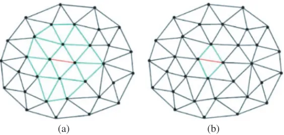
L to save the additional computational cost and guarantee a sparse R at most. In fact, even with a diagonal lumping L,R and T are denser thanK. For illustration purposes, here we take inter-related edges in 2-dimensional mesh for example. As shown in Figure 1, for the given edge highlighted in red, its associated edges highlighted in green in matrix T with diagonal lumping, shown in Figure 1(a), are typically more than their counterparts in matrix K, shown in Figure 1(b).
(a) (b)
Figure 1. Associated edges in (a) the matrixT with diagonal lumping; (b) the matrix K.
3. APPLICATIONS IN FREQUENCY AND TIME DOMAIN ANALYSIS
3.1. Low-Frequency Breakdown Problem in Frequency-Domain Full-Wave Analysis
The time-harmonic form ofA formulation (6) has the following form,
curlνcurlA−εgradχ−1divεA−ω2εA=J. (23) where ω is the working frequency. The finite element discretization of Eq. (23) leads to the following
equation,
K+R−ω2Mξ=ζ. (24) Compared with the conventional full-wave analysis, the generalized Lorenz gauged A formulation (23) involves an additional term εgrad (χ−1divεA) which corresponds to R. By contrast, the finite element discretization of conventional E formulation gives rise to the following equation,
Gauss’s law is not taken into account since it is automatically satisfied in the case of high working frequency, provided that the imposed current excitation J is physically compatible, which is divJ = 0. However, numerical difficulty appears when the working frequency ω approaches zero. In this case, the divergence free constraint cannot be derived from the full-waveEformulation. Numerically, the positive semi-definite matrix K dominates the coefficient matrix, so the coefficient matrix K−ω2M becomes ill-conditioned and even singular. On the other hand, although the current J is physically compatible, the vector iωζ in Eq. (25) is probably incompatible in the discrete system of Eq. (25); in other words,
iωζ does not belong to the range of K. Therefore, the low-frequency breakdown happens. In Eq. (24), the null space of discrete double-curl operator K is removed by the introduction ofR. Therefore, the discrete system in Eq. (24) is positive definite in the range of low-frequency, and its condition number remains stable whenω tends to be zero.
3.2. Spurious Linear Growth Problem in Time-Domain Full-Wave Analysis
In the conventional time-domain full-wave analysis, there is a spurious linear growth in solution if the simulation is carried on long enough time. Consider a source-free problem and take E formulation for example,
curlνcurlE+ε∂t2E = 0. (26)
Assume thatE(t) is the physical solution of Eq. (26), then the solution,
E∗(t) =E(t) +tgradV, (27) also satisfies Eq. (26). It contains a non-physical solution tgradV which is curl-free in space corresponding to zero modes and grows linearly with respect to time in theory. Here we use formulation (6) to destroy the linear growth of spurious modes in numerical solution. By employing the compatible finite element method with diagonal lumping, we obtain the following ordinary differential equations,
[K+R]ξ+Mξ¨= 0, (28)
By means of the generalized Lorenz gauged formulation, spurious zero modes now become simple harmonic vibrations with finite periods. Compared with shifting frequency method [7], a merit of Eq. (28) is that it does not pollute physical modes when suppressing spurious zero modes. The spatially discrete system in Eq. (28) is integrated in time using the Newmark-β method with integration parameters β= 0.25 and γ = 0.5, and the fully discretized form can be derived as
0.25Δt2[K+R] +Mξn+1=−20.25Δt2[K+R]−Mξn−0.25Δt2[K+R] +Mξn−1. (29)
3.3. Solution of the Discrete Linear Systems
As we have mentioned above, K is positive semi-definite, and M is positive definite. Considering frequency-domain full-wave E formulation, when the working frequency ω is larger than zero, the coefficient matrix in Equation (25) becomes indefinite, so a MINRES solver, instead of the CG solver that only works for symmetric positive definite system, should be generally used. However, if ω is extremely low, Equation (25) probably leads to the breakdown of the MINRES solver. Fortunately, the coefficient matrix in Equation (24) is symmetric positive definite when frequency ω is very low including the limit case of zero, allowing us to use either CG method or MINRES method. By contrast, in time-domain analysis, instead of solving Equation (29) in every step, we calculate the inverse of the coefficient matrix once and obtain an explicit expression for transient solution as follows,
ξn+1 = 40.25Δt2[K+R] +M−1M ξn−2ξn−ξn−1. (30)
4. NUMERICAL EXAMPLES
4.1. Spectral Distributions
It is well known that the spectral properties of the discrete system matrix provide important insight in the convergence behavior of the Krylov subspace methods [2]. In this section, the condition numbers are mainly compared among those discrete systems by using different methods. Here a quarter of sphere cavity with radius 1 m is taken into account. The model filled with air is divided into tetrahedra with outer faces defined as a perfect electric conductor. Figure 2 shows that two situations involving uniform mesh and nonuniform mesh are considered. Table 1 gives the information of finite element models.
(a) (b)
Figure 2. Finite element models, (a) with uniform mesh; (b) with non-uniform mesh.
Table 1. The information of finite element models.
Tetrahedra Free edges Free nodes
Uniform mesh 4140 4940 723
Non-uniform mesh 2264 3216 584
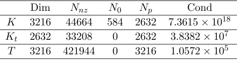
Here we denote the dimension of a matrix by “Dim”, the number of non-zero elements by “Nnz”,
and the number of nearly zero and positive eigenvalues by “N0” and “Np”, respectively. Tables 2 and 3 provide the spectrum statistics of the discrete double-curl operator K, the discrete tree gauged double-curl operator Kt, and the discrete Lorenz gauged double-curl operator T. As shown in Tables 2 and 3,
K is highly singular with the nullity ofN0, the number of free nodes. By contrast, the matrices Ktand
Table 2. Statistics of eigenvalues for the quarter sphere with uniform mesh.
Dim Nnz N0 Np Cond
K 4940 73424 723 4217 1.4206×10¹⁸
Kt 4217 56481 0 4217 2.4386×10⁵
T 4940 758230 0 4940 1.0592×10³
Table 3. Statistics of eigenvalues for the quarter sphere with non-uniform mesh.
Dim Nnz N0 Np Cond
K 3216 44664 584 2632 7.3615×10¹⁸
Kt 2632 33208 0 2632 3.8382×10⁷
T are both positive definite. We also investigate their condition numbers which are defined as follows,
Cond = max|λ|
min|λ|, (31)
where max|λ|and min|λ|are the maximum and minimum eigenvalues of a matrix. Generally, a small condition number is desired for a linear equation, which often indicates a rapid convergence of Krylov subspace methods. Tables 2–3 show the matrixT has minimum condition numbers. Figure 3 plots the spectrums of K, Kt and T of the model with non-uniform mesh. Furthermore, the condition numbers
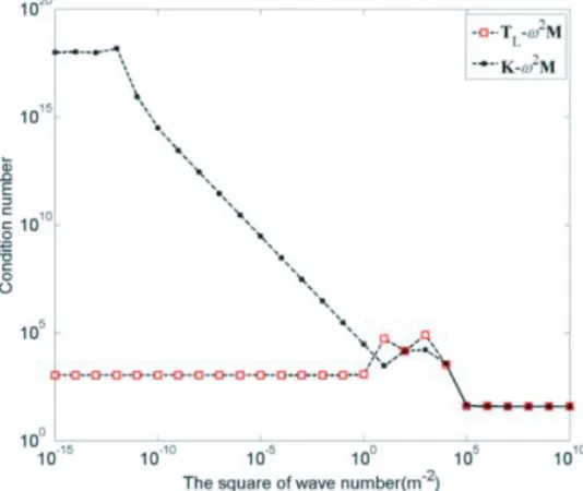
of the matricesT−ω2M andK−ω2M varying with the square of wave numberk2 =ω2μ0ε0in uniform mesh are investigated in Figure 4. The condition number of the matrix K −ω2M in conventional formulation becomes very large as k2 decreases. Therefore, a very little of incompatible excitation can lead to a bad convergence and inaccurate solution. Fortunately, this difficulty disappears in the generalized Lorenz gauged Aformulation. We can see that the condition number of T−ω2M is stable and bounded by 7.9764×10⁴. Especially, at the low-frequency band withk2 varying from 1×10⁻¹⁵m−2 to 1 m−2, the condition number only has a very little variation.
(a)
(b)
(c)
Figure 3. Spectral distribution of the finite element matrices with non-uniform mesh.
4.2. Low-Frequency Breakdown Problem of a Block Cavity
A block cavity 0.5 m×0.5 m×3 m, shown in Figure 5, is taken into consideration. The structure is partitioned into 2549 tetrahedra with 2949 free edges and 400 free nodes. There are the perfect electric conductors in the planes ofy= 0 m andy = 0.5 m. In the plane ofz= 3 m, the end of the block cavity, they component of E is set as 1 Vm. The exact solution of electric field intensity E in the cavity can thus be easily obtained: they component ofE along thex-axis is a sine curve with the period of 2πω−1
and the crest in the planez= 0 m. It can be used to verify numerical solutions.
Figure 5. The finite element model of the block cavity problem.
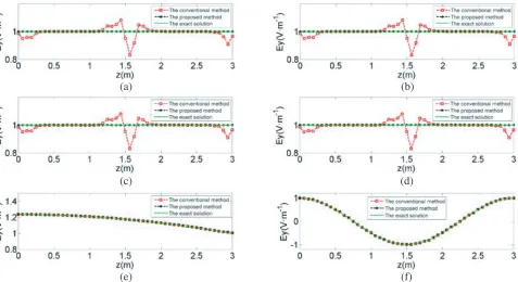
In this example, when using conventional full-wave formulation, although MINRES converges within iteration criterion at all given frequency points, low-frequency inaccuracies arise in numerical solutions. Figure 6 plots the distributions of theycomponent of E along the middle line in positivexdirection of the model. Clearly, at the frequency below 1.0×10⁵Hz, the wave profiles are distorted. By contrast, the numerical solutions by using the compatible discrete regularization method are consistent with exact solutions. Setting the tolerance 1.0×10⁻⁸ and maximum number of iteration 1000, Table 4 provides the solution information in terms of iteration counts and time at different frequency ranging from 0 Hz to 1×10⁸Hz. The number of iterations is almost unchanged from 0 Hz to 1×10⁸Hz. Furthermore, due to the symmetric positive definite property ofT −ω2M in a wide range of frequency, CG method is also an alternative solver. However, in every iteration, MINRES or CG method generally costs more time in formulation (24) because T−ω2M is denser thanK−ω2M.
(a) (b)
(c) (d)
(e) (f)
Table 4. Iteration counts and time for the block cavity problem at different frequencies.
FREQ(Hz) 1×10⁸ 1×10⁷ 1×10⁵ 1×10³ 10 0
SOLVER MR CG MR CG MR CG MR CG MR CG MR CG
K IC 527 - 607 - 204 - 201 204 201 204 201 205
IT(s) 0.14 - 0.15 - 0.05 - 0.05 0.05 0.05 0.05 0.05 0.05
T IC 212 - 208 212 207 211 207 211 206 210 207 210
IT(s) 0.13 - 0.11 0.11 0.12 0.11 0.11 0.11 0.11 0.11 0.11 0.11
4.3. Low-Frequency Breakdown Problem Excited by a Cylindrical Current
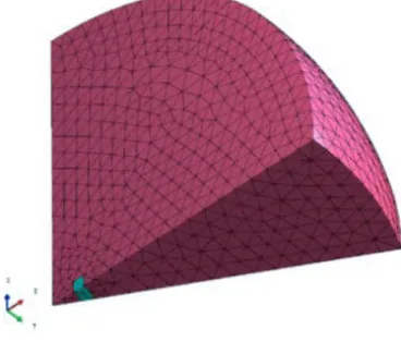
In this example, a simple cylindrical coil with imposed current 1 Am−2 is placed in the center of a spherical volume which is backed by perfect electric conductor, as shown in Figure 7. The permittivity and permeability in this model are the same as in air. The height, inner and outer diameters of the cylinder coil are 0.08 m, 0.08 m and 0.12 m, respectively, and the radius of the sphere volume is 1 m. Because the structure is symmetric, to save the computation cost, only a twelfth part, instead of the whole domain, is analyzed. The tolerance is 1.0×10⁻⁸, and the maximum number of iteration is 2000.
Figure 7. The finite element model of the cylindrical coil problem.
Table 5 shows that the conventional formulation (25) encounters divergence under current excitation. At the frequency below 1.0×10⁵Hz, MINRES and CG methods both fail to converge within the maximum number of iteration. However, formulation (24) is rather robust at the whole given frequency band with the use of the MINRES method; it has no breakdown problem with decreasing frequency, possessing stable numerical performance in terms of iteration counts and time. On the other hand, it is amazing that even when the frequency has been as large as 1.0×10⁸Hz with apparent wave phenomenon in the cavity, there is no apparent increase of iteration counts and time with the
Table 5. Iteration counts and time of the cylindrical coil problem at different frequencies.
FREQ(Hz) 4×10⁸ 1×10⁸ 1×10⁷ 1×10⁵ 1×10³
SOLVER MR CG MR CG MR CG MR CG MR CG
K IC 1712 - 1153 - 1508 - - - -
-IT(s) 2.65 - 1.29 - 1.43 - - - -
-T IC 569 - 317 329 304 319 304 319 303 320
use of MINRES in formulation (24). Furthermore, CG is also available for formulation (24) at a broad low-frequency band.
Because the mixed finite element method has been proved stable and well-posed in time-harmonic electromagnetic problems, here we use its results to verify the accuracy of the conventional method and t proposed method. Figure 8 plots the distributions of they component of imaginary electric field intensityE along thex-axis at different frequencies. It indicates that the result of the proposed method is consistent with that of the mixed finite element method even at extremely low frequency. However, the conventional method is reliable at high-frequency band but fails to predict electromagnetic fields at low-frequency band.
(a) (b) (c)
Figure 8. The distribution of they component of imaginary electric field intensity along thex-axis at the frequencies of 1×10³Hz, 1×10⁷Hz, and 4×10⁸Hz.
4.4. Magnetostatic Problem of Cylinder Coil around a Cylinder Iron
Here an example of an iron cylinder with an assumed relative permeability 1000, shown in Figure 9(a), is presented to verify the generalized Lorenz gauged formulation used in magnetostatic problems [16, 18]. The current density is assumed 1×10⁶Am−2. Considering the symmetry of the model, only one eighth of the model is taken into account. The model is divided into 66558 tetrahedra consisting of 75978 free edges and 10483 free nodes. The no gauged formulation, generalized Lorenz gauged formulation and tree gauged formulation are all applied to solve this problem. For the tree gauged formulation, the degree of
(a) (b)
freedoms are reduced to 65495; however, it worsens the condition number and thus more iterations are required. By contrast, the generalized Lorenz gauged formulation has an improved condition number but with denser matrix.
The no gauged formulation cannot converge to a solution with the use of CG method, whereas the tree gauged formulation and generalized Lorenz gauged formulation both converge. Figure 9(b) plots and compares the z-component of the magnetic flux density along the x-axes using the tree gauged formulation and generalized Lorenz gauged formulation. These results of magnetic flux density are in overlap agreement with each other, which demonstrates the accuracy of the generalized Lorenz gauged formulation. However, those two formulations show different numerical performances. Table 6 gives iteration information including the counts and times. The generalized Lorenz gauged formulation spends more time than the tree gauged formulation in each iteration because of its less sparsity, but needs fewer iterations due to improved condition number. On balance, the generalized Lorenz gauged formulation is more efficient than the tree gauged formulation in this example.
Table 6. Iteration counts and time of the magnetostatic problem.
K IC
-IT(s)
-Kt IT(s)IC 168.4046468
T IC 3776
IT(s) 76.21
4.5. Spurious Linear Growth Problem Excited by an Initialized Field
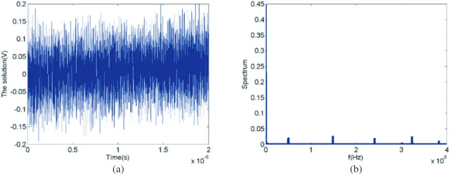
Here a block cavity model, having the same geometry of Figure 5, is used to illustrate the suppression of the spurious linear growth problem in time-domain analysis. The spurious linear growth generally exists in the transient analysis, though sometimes it is not noticeable in limited computational time. Once the curl-free distribution is generated, the spurious solution will linearly increase with time no matter how small it is at the initialized moment.
In this example, a coarser mesh is adopted for the model to reduce the computation cost. The planes y = 0 m, y = 0.5 m, z = 0 m, and z = 3 m are the perfect electric conductors. The initialized field E0 = (0 Vm−1, 0 Vm−1, 1 Vm−1) and d2E0/dt2 = (0 Vm−1s−2, 0 Vm−1s−2,−5×10¹⁶Vm−1s−2)
(a) (b)
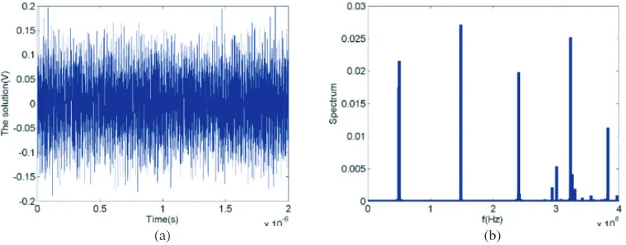
is set up at the middle plane of the block. The time step and total number of steps are set as 1×10⁻⁹s and 216, respectively. Figure 10(a) plots the time-varying solution of one edge at the middle plane computed by the conventional method, clearly showing that there is a spurious linear growth in the solution. Moreover, the spectrum of the solution, as shown in Figure 10(b), also reveals the non-physical zero modes are involved in the transient solution. To suppress the spurious solution, we apply the generalized Lorenz gauged formulation to solve this problem. Figure 11(a) shows the spurious linear growth phenomenon disappears with the use of the generalized Lorenz gauged formulation. The spectrum distribution in Figure 11(b) also indicates that those non-physical zero modes are completely removed.
(a) (b)
Figure 11. The solution in time-domain and its frequency spectrum using the proposed method.
5. CONCLUSIONS
In this paper, we introduce diagonal lumping in generalized Lorenz gauged charge-freeAformulation. In this formulation, the discrete double-curl operator is transferred to a discrete quasi-Laplacian operator with improved condition number. Compared with using SAI for the inverse of mass matrix, the diagonal lumping can save computation cost and guarantee a sparser coefficient matrix.
The formulation with diagonal lumping is applied in the frequency-domain full-wave analysis to overcome the low-frequency breakdown problem. It is shown that the formulation is more accurate and robust than conventional method at low-frequency band, including the limit case of magnetostatic field. Moreover, it can also be used in the time-domain full-wave analysis to suppress the spurious linear growth problem arising in conventional method.
ACKNOWLEDGMENT
This paper is accomplished with support from the National Natural Science Foundation of China (11272074) and the National Science and Technology Major Project (2011ZX02403-004).
REFERENCES
1. Jin, J. M.,The Finite Element Method in Electromagnetics, 3rd Edition, John Wiley & Sons, New York, 2015.
3. Lee, S. H. and J. M. Jin, “Application of the treecotree splitting for improving matrix conditioning in the full-wave finite-element analysis of high-speed circuits,” Microwave and Optical Technology Letters, Vol. 50, No. 6, 1476–1481, 2008.
4. Zhu, J. and D. Jiao, “A theoretically rigorous full-wave finite-element-based solution of Maxwell’s equations from DC to high frequencies,”IEEE Transactions on Advanced Packaging, Vol. 33, No. 4, 1043–1050, 2010.
5. Zhu, J. and D. Jiao, “A rigorous solution to the low-frequency breakdown in full-wave finite-element-based analysis of general problems involving inhomogeneous lossless/lossy dielectrics and nonideal conductors,” IEEE Transactions on Microwave Theory and Techniques, Vol. 59, No. 12, 3294–3306, 2011.
6. Venkatarayalu, N. V., M. N. Vouvakis, Y. B. Gan, et al., “Suppressing linear time growth in edge element based finite element time domain solution using divergence free constraint equation,”
Antennas and Propagation Society International Symposium, 193–196, 2005.
7. Hwang, C. T. and R. B. Wu, “Treating late-time instability of hybrid finite-element/finite-difference time-domain method,”IEEE Transactions on Antennas and Propagation, Vol. 47, No. 2, 227–232, 1999.
8. Golias, N. A. and T. D. Tsiboukis, “Magnetostatics with edge elements: A numerical investigation in the choice of the tree,”IEEE Transactions on Magnetics, Vol. 30, No. 5, 2877–2880, 1994. 9. Kikuchi, F., “Mixed and penalty formulations for finite element analysis of an eigenvalue problem
in electromagnetism,” Computer Methods in Applied Mechanics and Engineering, Vol. 64, No. 1, 509–521, 1987.
10. Chen, Z., Q. Du, and J. Zou, “Finite element methods with matching and nonmatching meshes for Maxwell equations with discontinuous coefficients,”SIAM Journal on Numerical Analysis, Vol. 37, No. 5, 1542–1570, 2000.
11. Benzi, M., G. H. Golub, and J. Liesen, “Numerical solution of saddle point problems,”
Actanumerica, Vol. 14, 1–137, 2005.
12. Bespalov, A. N., “Finite element method for the eigenmode problem of a RF cavity resonator,”
Russian Journal of Numerical Analysis and Mathematical Modelling, Vol. 3, No. 3, 163–78, 1988. 13. Hiptmair, R., “Finite elements in computational electromagnetism,” Acta Numerica, Vol. 11, 237–
339, 2002.
14. Chew, W. C., “Vector potential electromagnetics with generalized gauge for inhomogeneous media: Formulation,” Progress In Electromagnetics Research, Vol. 149, 69–84, 2014.
15. Li, Y. L., S. Sun, Q. I. Dai, et al., “Finite element implementation of the generalized-Lorenz gaugedA-Φ formulation for low-frequency circuit modeling,”IEEE Transactions on Antennas and Propagation, Vol. 64, No. 10, 4355–4364, 2016.
16. Li, Y. L., S. Sun, Q. I. Dai, and W. C. Chew, “Vectorial solution to double curl equation with generalized coulomb gauge for magnetostatic problems,”IEEE Transactions on Magnetics, Vol. 51, No. 8, 1–6, 2015.
17. Bossavit, A. and L. Kettunen, “Yee-like schemes on a tetrahedral mesh, with diagonal lumping,”
International Journal of Numerical Modelling Electronic Networks Devices and Fields, Vol. 12, 129–142, 1999.