An ADE-TLM Modeling of Biological Tissues with Cole-Cole
Dispersion Model
Mohammed Kanjaa*, Khalid Mounirh, Soufiane El Adraoui, Otman El Mrabet, and Mohsine Khalladi
Abstract—In this paper, an auxiliary differential equation (ADE) transmission line method (TLM) is proposed for broadband modeling of electromagnetic (EM) wave propagation in biological tissues with the Cole-Cole dispersion Model. The fractional derivative problem is surmounted by assuming a linear behavior of the polarization current when the time discretization is short enough. The polarization current density is approached using Lagrange extrapolation polynomial, and the fractional derivation is obtained according to Riemann definition of a fractional α-order derivative. Reflection coefficients at an air/muscle and air/fat tissues interfaces simulated in a 1-D domain are found in good agreement with those obtained from the analytic model over a broad frequency range, demonstrating the validity of the proposed approach.
1. INTRODUCTION
In the last two decades there has been a renewed interest in the interaction between biological tissues and electromagnetic field at microwave frequencies due to new promising applications of this technology in biomedical engineering. Applications, like microwave imaging [1, 2], minimal invasive cancer therapies as thermal ablations [3], ultra-wide band temperature dependent dielectric spectroscopy [4], and EM dosimetry [5], rely heavily on an accurate mathematical model of these tissues behavior while interacting with the electromagnetic field. Numerical resolution of the propagation problem within these tissues requires previous incorporation of the dielectric data at all the working frequencies.
A first model of the time response in a time varying electric field of biological tissues was formulated by Debye [6] through a time decaying polarization currentj(t) = ∂P∂t resulting from the time variation of polarization vectorP(t). This model, even if it fits the experimental results in liquids, loses its accuracy when being applied over a large band of frequency or in the presence of more than one type of polar molecule. This non-Debye relaxation is attributed to the existence of different relaxation processes [7], each with its own relaxation time τ and its amplitude Δ. Therefore, a more accurate description of this behavior is then given by the sum of the individual relaxation processes leading to a multipole model. However, in the case of the biological tissue, there is a multiple contributions to each relaxation process resulting in a broadening of the relaxation zone. Cole and Cole [7] proposed an Argand diagram in which the imaginary part of the complex permittivity r is plotted as a function of its real part
following the empirical relation:
r(ω) =∞+
p
p=1
Δp
1 + (jωτp)αp (1)
where∞ is the optical relative permittivity, Δp =s−∞the amplitude of thep-th pole,s the static
relative permittivity, ω the angular frequency, τp the relaxation time, αp the parameter that indicates
Received 12 November 2019, Accepted 15 January 2020, Scheduled 3 February 2020
* Corresponding author: Mohammed Kanjaa ([email protected]).
the broadening of the dispersion for this pole, which in the Cole-Cole model must satisfy 0 < αp <1, and in the case of αp = 1 the model is simplified to a Debye dispersion problem and j = √−1. The
difficulty in the numerical implementation of such a model arises from the αp parameter which is a
non-integer. The consequence is a fractional order differentiation in the time domain which is more challenging than the Debye time domain solution. To address this problem, the authors in [8] used the Letnikov fractional derivative by introducing a Stirling asymptotic formula and a recursive relation for the polarization vector. The computational demands of the FDTD scheme were considerably reduced, but it required the storage of a large number of previous values of the polarization vector. In [9], the authors used the Z transform to formulate the frequency dependence between the electric flux density and the electric field, and the fractional derivative was approximated by using a polynomial method. Rekanos et al. [10] used the Pade approximation, where the fractional power term is approximated using a Pade technique. All the latter approximations were made in the context of the FDTD method.
The TLM method, even if it is flexible, wide band, and a time domain method, cannot deal with the dispersive aspect of the Cole-Cole medium directly. In [11], an approach based on a convolution product between the susceptibility and the electric field and the temporal behavior is deduced by a DFT and a non-recursive summation leading to a considerable computational cost and a non-negligible error at high frequencies. The causality principle is used to justify the minor dependence of the recent susceptibility values on previous ones, but the problem of the fractional Differentegration was not addressed.
The use of an ADE algorithm in TLM method has been proven efficient for dispersive media [12]. To the best of our knowledge, this technique has not been used before to solve the fractional derivative problem in the TLM method. In order to bypass this shortcoming, we present in this work an ADE-TLM algorithm to model the Cole-Cole dispersion. The polarization current density is approached using an extrapolation with Lagrange polynomial method, and the fractional derivation is obtained using the Riemann definition of the α-order derivative. The auxiliary differential equation is used to establish the update equation of the polarization currents which are included later in the general structure of the SCN-TLM node.
2. FORMULATION AND EQUATIONS
In the Cole-Cole model, the relationship between the polarization current related to the pth pole and the electric field is given by:
Jp(ω) =0Δp1 + (jω
jωτp)αpE(ω) (2)
where (jωτp)αp is the power law function of frequency which in time domain results in a fractional
derivative of orderα:
Jp(t) +ταpDαpJp(t) =0Δp∂E(t)
∂t (3)
One could consider an analytic solution for this equation, but due to the fractional derivative, this can only be done for particular values of αp, hence a numerical solution is necessary with a previous discretization of the temporal values of the vectors.
In order to obtain the descritized expression of Jp(t), the polarization current vector can be approached using a Lagrange interpolation in the time intervalti < t < tj with cardinal functions:
Li(t) = n
j=1;i=j
(t−tj)
(ti−tj) (4)
the interpolated expression ofJp(t) is then obtained:
Jp(t) =
n
i=1
JiLi(t) (5)
and by applying Eq. (4) in the time intervalnΔt < t <(n+ 1)Δt we obtain the cardinal functions:
Ln(t) = t−(n+ 1)Δt
nΔt−(n+ 1)Δt Ln+1(t) =
t−nΔt
By substituting Eq. (6) in Eq. (5), the polynomial extrapolation of the polarization current density between time steps nΔtand (n+ 1)Δt can be found in a straightforward manner as follows:
Jp(t) = t−(n+ 1)Δt
nΔt−(n+ 1)ΔtJ n
p + (n+ 1)Δt−ntΔ−tnΔtJnp+1 (7)
which after simplification can be rewritten as:
Jp(t) = J
n+1
p −Jnp
Δt t+ (n+ 1)J n
p −nJnp+1 (8)
Furthermore, by substituting Eq. (8) into Eq. (3), we derive the auxiliary differential equation with a fractional order derivative given by:
Jnp+1+Jnp
2 +τ
αpJ
n+1
p −Jnp
Δt D
αpt+Dαp((n+ 1)Jn
p −nJnp+1) =0Δp∂E
∂t (9)
The generalization of the derivation operator to arbitrary non-integer orders has been subject to intensive research from mathematicians [13, 14] and in electromagnetism [15]. One of the definitions in [16] for the fractional derivative, symbolized by the operator Dαx, is given for the power series with fractional exponents by considering a functionh(x) defined as a power seriesh(x) =ni=1Ai(x−a)ν+i/n
forν >−1 andna positive integer, so each term (x−a)p could have a non-integer exponentp=ν+i/n, then according to Reimann [15] a fractional derivative of order α for this term is given by:
Dxα(x−a)p = d
α(x−a)p
d(x−a)α =
Γ(p+ 1)
Γ(p−α+ 1)(x−a)
p−α f or x > a (10)
where in our caseα is a non-integer number [17].
Hence by applying the fractional derivation operator given in (9) to (10) and forp= 1 and a= 0, we obtain:
Jnp+1+Jnp
2 +τ
αpJ
n+1
p −Jnp
Δt
0.5 Γ(2−αp)t
1−αp+((n+ 1)Jnp −nJn +1
p )
Γ(1−αp) t
−αp =
0Δp
En+1−En
Δt (11)
from which the update equation for the polarization current is derived:
Jnp+1 =−φp
ψpJ n p +ψζp
p(E
n+1−En) (12)
where the update parametersψp,φp and ζp are:
ψp = 12 +τ αp
p
Δt
Γ(2) Γ(2−αp)t
1−αp−
n τ
αp
p
Γ(1−αp)t
−αp (13)
φp = 12 −τ αp
p
Δt
Γ(2) Γ(2−αp)t
1−αp+ (n+ 1) τ
αp
p
Γ(1−αp)t
−αp (14)
ζp = 0Δp
Δt (15)
To get the update equation of the electric field components, we start from the Maxwell-Ampere equation, and by including the conductivity term:
∇ ×H=0∞∂
E
∂t +σ0E+ p
p=1
Jp (16)
whereσ0 is the static ionic conductivity, and Eq. (16) formulated at time step n+12 gives:
(∇ ×H)n+12 =0∞E
n+1−En
Δt +σ0
En+1+En
2 +
p
p=1
Jn+ 1 2
and by approaching Jn+12 by the average of its values at time steps nand n+ 1
Jnp+12 = J
n+1
p +Jnp
2 (18)
Finally, the updated electric field is given by:
Ex,y,zn+1 = Enx,y,z
1−2σ0Δt
D
−
p
(1−φψp
p)Δt
D J
n
px,y,z+ 2ΔDt(∇ ×H)n+
1 2
x,y,z (19)
D = 20∞+
p ζpΔt
ψp +σ0Δt (20)
3. THE TLM FORMALISM
The TLM method is a numerical technique based on the discretization of the computational domain according to Huygens principle as an alternative to the Maxwell equations used in the FDTD method [18]. In this method, the simulation domain is discretized in cells where a series of uniform transmission lines, parallel and series stubs, and additional sources are used to take account of the real characteristics of the propagation through the medium as given by Maxwell equations. Therefore, instead of electric and magnetic field components the electromagnetic field is represented by voltage and current waves, propagating through the unit cell circuit referred to as symmetrical condensed node (SCN). The relationship between the electromagnetic field and the voltage and current waves at the time step nΔt and at the center of the node are formulated as follows [19].
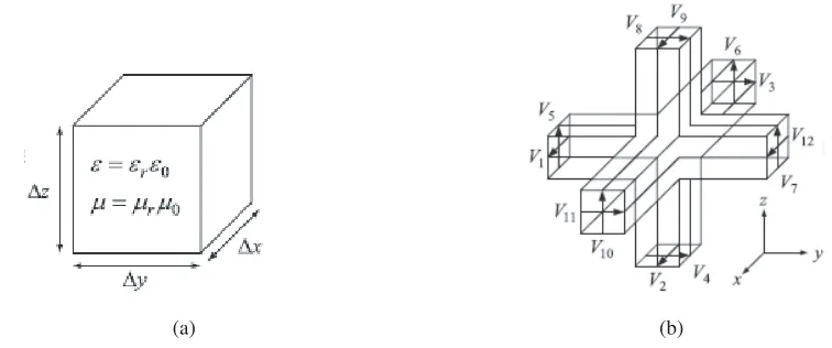
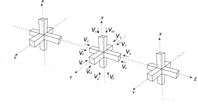
As can be seen in Figure 1(b), the SCN consists of interconnected transmission lines. This structure models a unit cell of the propagation medium as in Figure 1(a). Each face of the cell corresponds to two ports orthogonal to each other and labeled from 1 to 12. These stubs model the propagation through free space and have therefore its characteristic impedance Z0 =√0μ0. Three additional open circuit (13, 14, 15) stubs must be added to the node to account for the dispersive behavior of the medium. The SCN nodes are connected to each other to form the simulation domain given in Figure 2 for a 1-D propagation.
(a) (b)
Figure 1. Structure of the TLM symmetrical condensed node, (a) unit volume of the dielectric material, (b) equivalent SCN.
The relationship between the electromagnetic field and the voltage and current waves at the time step nΔt and at the center of the node are formulated as follows [19]:
Ex,y,zn = V
n x,y,z
Δl H n x,y,z= I
n x,y,z
Figure 2. Structure of the 1-D SCN grid used in this work to model the simulation domain.
In this algorithm as in [11, 12, 20], the dispersive properties of the medium are accounted for by adding voltage sources sV to each node, and these sources constitute the counterparts of the terms in the FDTD formulation that have no equivalents in the TLM formalism. Therefore, the voltage at the center of the node, as deduced from the conservation laws [21], becomes:
Vx,y,zn+1 =Vx,y,zn + 1
4 +Yocx,y,z(sV n+1
x,y,z+sVx,y,zn ) +4 +Y4 ocx,y,z
ΔlΔt 0
(∇ ×H)n+12
x,y,z (22)
whereYocx,y,z indicates the normalized admittance of the open circuit stub added to the node.
When being expressed in terms of incident voltages on the corresponding stubs and accounting for the voltage sources injected in the stubs (16, 17, 18) to complete the model of the Cole-Cole medium:
Vx,y,zn+1 = 2 4 +Yox,y,z
V1i,3,5+V2i,4,6+V9i,8,7+V12i,11,10+Yoc,x,y,zV13i,14,15+ 1 2sV
n+1 16,17,18
(23)
where subscript iindicates the incident pulses on the indicated stubs.
In the TLM formalism, the update equation issued from the ADE in the Eq. (12) becomes:
Jpx,y,zn+1 =−φp
ψpJ n
px,y,z+ψζp pΔl(V
n+1
x,y,z−Vx,y,zn ) (24)
and the electric field update equation obtained in Eq. (19) is also formulated in the TLM formalism as:
Vx,y,zn+1=Vx,y,zn
1−2σ0Δt
D
−
p
(1−ψφp
p)ΔtΔl
D J
n px,y,z+
2ΔtΔl
D (∇ ×H) n+12
x,y,z (25)
Using the analogy between Eqs. (22) and (25), the expression of the normalized admittance of the stub added to the SCN node is obtained straightforwardly:
Yoc= 4
D
20 − 1
(26)
and the update equation for voltage sources at the center of the node:
sVx,y,zn+1=−sVx,y,zn −4σ0Δt
0 V
n x,y,z−
p
2(1− φψp
p)ΔtΔl
0 Jpx,y,z
(27)
that can be simplified to
sVx,y,zn+1 =−sVx,y,zn +C1Vx,y,zn +
p
with update constants:
C1 = − 4σ0Δt
0
(29)
C2p = −
2(1−φψp
p)ΔtΔl
0
(30)
A final step to establish the TLM formulation is to express the scattering process on the capacitive stubs:
V13r,14,15
n
= [Vx,y,z]n− V13i,14,15
n
(31)
4. SIMULATION AND RESULTS
In order to verify the new proposed algorithm, a one-dimensional problem is simulated, where a Cole-Cole medium (fat or muscle) occupies the region z ≥ 0, while the rest of space is air. The incident wave is a derivative Gaussian pulse given by −→Einc = (t−tτ20)exp(−4π((t−t0)
2
τ2 ) ˆex where t0 = 200Δt and
τ = 220Δt polarized in thex direction, and propagates along thez axis. In the TLM implementation, the considered 1-D simulation domain (see Figure 3) consists of a grid of 1000 cells interconnected on the z axis as in Figure 2, 500 of which were used to model the Cole-Cole medium, and the remaining cells were used to model the air. The cell dimension Δl satisfies the stability condition Δt = Δl/2c, and the time step is set as Δt= 0.125 ps. The simulation domain is truncated by an unsplit PML layer [22] of 10 cells at the beginning and the end.
Figure 3. 3D view of the computation domain of a normal incidence on an air/Cole-Cole medium, incident and reflected fields are calculated at point P.
The fourth order Cole-Cole parameters for fat tissue as well as muscle tissue are listed in Table 1 [9]. The values of the electric field are recorded at a point P located at the center of the SCN node 10 cells before the air-medium interface. Figure 4(a) shows the incident impulse at iteration 399 propagating in the air, and Figure 4(b) at iteration 927 depicts the reflected and transmitted impulse on the the air/muscle interface.
Table 1. Cole-Cole constants for tissues of muscle and fat
Tissue ∞ σ0 Δ1 τ1(ps) α1 Δ2 τ2 (ps) α2 Δ3 τ3 (µs) α3 Δ4 τ4 (ps) α4
Muscle 2.5 0.035 9 7.96 0.8 35 15.92 0.9 3.3E4 159.15 0.95 1.0E7 15.915 0.99
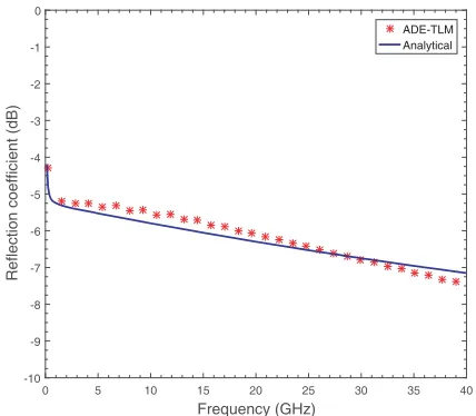
In Figures 5 and 6, the simulation results for both cases (fat and muscle) are compared to the theoretical reflection at the air/Cole-Cole medium interface which can be obtained by using the following equation [23]:
|R|= |1−
√ r |
|1 +√r | (32)
A good agreement over the whole frequency band is observed. The slight discrepancy between the numerical and theoretical results can be ascribed first to the numerical dispersion characteristic to the TLM method which is less than the standard FDTD method [24], then to the approximation made to the polarization current value when performing the Lagrange extrapolation on each iteration [25]. Therefore, even with this small shift, the proposed approach requires a simple precalculation for the fractional derivative operator as opposed to other methods [11] which makes it effective and easy to implement.
0 200 400 600 800 1000
TLM cells -1
-0.8 -0.6 -0.4 -0.2 0 0.2 0.4 0.6 0.8 1
Impulse amplitude (V/m)
Time step = 399
Air Cole-Cole medium
(a)
0 200 400 600 800 1000
TLM cells -1
-0.8 -0.6 -0.4 -0.2 0 0.2 0.4 0.6 0.8 1
Impulse amplitude (V/m)
Time step = 927
Air Cole-Cole medium
(b)
Figure 4. Propagation of an incident derivative Gaussian pulse through Cole-Cole medium model of human muscle, (a) at iteration 399 (incident pulse), (b) at iteration 677 (reflected and transmitted pulse).
0 5 10 15 20 25 30 35 40
Frequency (GHz)
-4 -3.5 -3 -2.5 -2 -1.5 -1 -0.5 0
Reflection coefficient (dB)
ADE-TLM Analytical
Figure 5. Reflection coefficient (dB) at normal incidence on an air/Muscle interface.
0 5 10 15 20 25 30 35 40
Frequency (GHz)
-10 -9 -8 -7 -6 -5 -4 -3 -2 -1 0
Reflection coefficient (dB)
ADE-TLM Analytical
5. CONCLUSION
In this paper, an ADE-TLM formulation is presented to study the electromagnetic wave propagation in biological tissues using Cole-Cole dispersion model. The fractional-order derivative in the Cole-Cole model is tackled by using a polynomial extrapolation of the polarization current. This approximation considerably reduces the numerical cost of the simulation since only two previous values of J field are needed at each iteration. The calculations complexity is also reduced by performing a Reimann derivation on the obtained polynomial extrapolation of the polarization current. The presented results indicate the accuracy of our approach.
REFERENCES
1. Martellosio, A., M. Pasian, M. Bozzi, L. Perregrini, A. Mazzanti, F. Svelto, P. E. Summers, G. Renne, and M. Bellomi, “0.5–50 GHz dielectric characterisation of breast cancer tissues,”
Electronics Letters, Vol. 51, No. 13, 974–975, 2015.
2. Gavazzi, S., P. Limone, G. De Rosa, F. Molinari, and G. Vecchi, “Comparison of microwave dielectric properties of human normal, benign and malignant thyroid tissues obtained from surgeries: A preliminary study,”Biomedical Physics&Engineering Express, Vol. 4, No. 4, 047 003, 2018.
3. Ruvio, G., J. Eaton-Evans, A. Shahzad, and M. O’Halloran, “Numerical evaluation of microwave thermal ablation to treat small adrenocortical masses,”International Journal of RF and Microwave Computer-Aided Engineering, Vol. 28, No. 3, e21236, 2018.
4. Ley, S., S. Schilling, O. Fiser, J. Vrba, J. Sachs, and M. Helbig, “Ultra-wideband temperature dependent dielectric spectroscopy of porcine tissue and blood in the microwave frequency range,”
Sensors, Vol. 19, No. 7, 1707, 2019.
5. Chakarothai, J., K. Wake, and S. Watanabe, “Convergence of a single-frequency FDTD solution in numerical dosimetry,”IEEE Transactions on Microwave Theory and Techniques, Vol. 64, No. 3, 707–714, 2016.
6. Debye, P., “Part i. Dielectric constant. energy absorption in dielectrics with polar molecules,”
Transactions of the Faraday Society, Vol. 30, 679–684, 1934.
7. Cole, K. S. and R. H. Cole, “Dispersion and absorption in dielectrics i. Alternating current characteristics,” The Journal of Chemical Physics, Vol. 9, No. 4, 341–351, 1941.
8. Rekanos, I. T. and T. V. Yioultsis, “Approximation of Gr¨unwald-Letnikov fractional derivative for FDTD modeling of Cole-Cole media,” IEEE Transactions on Magnetics, Vol. 50, No. 2, 181–184, 2014.
9. Guo, B., J. Li, and H. Zmuda, “A new FDTD formulation for wave propagation in biological media with Cole-Cole model,”IEEE Microwave and Wireless Components Letters, Vol. 16, No. 12, 633–635, 2006.
10. Rekanos, I. T. and T. G. Papadopoulos, “An auxiliary differential equation method for FDTD modeling of wave propagation in Cole-Cole dispersive media,” IEEE Transactions on Antennas and Propagation, Vol. 58, No. 11, 3666–3674, 2010.
11. Barba, I., A. C. L. Cabeceira, M. Panizo, and J. Represa, “Modelling dispersive dielectrics in TLM method,”International Journal of Numerical Modelling: Electronic Networks, Devices and Fields, Vol. 14, No. 1, 15–30, 2001.
12. Mounirh, K., S. El Adraoui, Y. Ekdiha, M. Iben Yaich, and M. Khalladi, “Modeling of dispersive chiral media using the ADE-TLM method,” Progress In Electromagnetics Research M, Vol. 64, 157–166, 2018.
13. Samko, S. G., A. A. Kilbas, O. I. Marichev, et al.,Fractional Integrals and Derivatives, Vol. 1993, Gordon and Breach Science Publishers, Yverdon Yverdon-les-Bains, Switzerland, 1993.
15. Engheta, N., “On the role of fractional calculus in electromagnetic theory,” IEEE Antennas and Propagation Magazine, Vol. 39, No. 4, 35–46, Aug. 1997.
16. Engheta, N., “On fractional calculus and fractional multipoles in electromagnetism,” IEEE Transactions on Antennas and Propagation, Vol. 44, No. 4, 554–566, Apr. 1996.
17. Wharmby, A. W. and R. L. Bagley, “The application of the fractional calculus model for dispersion and absorption in dielectrics in terahertz waves,” International Journal of Engineering Science, Vol. 93, 1–12, 2015.
18. Jin, H. and R. Vahldieck, “Direct derivations of TLM symmetrical condensed node and hybrid symmetrical condensed node from Maxwell’s equations using centered differencing and averaging,”
IEEE Transactions on Microwave Theory and Techniques, Vol. 42, No. 12, 2554–2561, Dec. 1994. 19. Christopoulos, C., The Transmission-Line Modeling (TLM) Method in Electromagnetics, Morgan
& Claypool, 2006.
20. Cabeceira, A. C. L., I. Barba, A. Grande, and J. Represa, “A 2D-TLM model for electromagnetic wave propagation in chiral media,” Microwave and Optical Technology Letters, Vol. 46, No. 2, 180–182, 2005.
21. Yaich, M. I. and M. Khalladi, “The far-zone scattering calculation of frequency-dependent materials objects using the tlm method,”IEEE Transactions on Antennas and Propagation, Vol. 50, No. 11, 1605–1608, Nov. 2002.
22. Yaich, M. I., M. Kanjaa, S. E. Adraoui, K. Mounirh, and M. Khalladi, “An unsplit formulation of the 3D-PML absorbing boundary conditions for TLM-method in time domain,” 2018 6th International Conference on Multimedia Computing and Systems (ICMCS), 1–5, May 2018. 23. Taflove, A. and S. C. Hagness,Computational Electrodynamics: The Finite-difference Time-domain
Method, Artech House, 2005.
24. Juntunen, J. S. and T. D. Tsiboukis, “Reduction of numerical dispersion in fdtd method through artificial anisotropy,” IEEE Transactions on Microwave Theory and Techniques, Vol. 48, No. 4, 582–588, 2000.