An Inverse Electromagnetic Scattering Problem for an Ellipsoid

An Inverse Electromagnetic Scattering Problem for an Ellipsoid

Evangelia S. Athanasiadou, Stefania Zoi*, and Ioannis Arkoudis

Abstract—The scattering problem of time-harmonic electromagnetic plane waves by an impedance and a dielectric ellipsoid is considered. A low-frequency formulation of the direct scattering problem using the Rayleigh approximation is described. Considering far-field data, an inverse electromagnetic scattering problem is formulated and studied. A finite number of measurements of the leading-order term of the electric far-field pattern in the low-frequency approximation leads to specify the semi-axes of the ellipsoid. The orientation of the ellipsoid is obtained by using the Euler angles. Corresponding results for the sphere, spheroid, needle, and disc can be obtained considering them as geometrically degenerate forms of the ellipsoid for suitable values of its geometrical parameters.

1. INTRODUCTION

The inverse scattering theory has a lot of important applications in medical imaging, geological studies, and detection of buried or underwater objects. An ellipsoid can be considered as a good approximation for the shape of many objects such as spheres, spheroids, needles, and discs. Therefore, inverse scattering problems for ellipsoids are significant.

In a series of papers, Dassios and his coauthors have published results about ellipsoids in inverse scattering problems using far-field data and specifically the low frequency coefficients of the far-field patterns and the scattering cross-sections. Dassios in [6] first introduced a new method for solving inverse scattering problems for an acoustically soft ellipsoid. Later, similar problems were studied for a rigid and a penetrable ellipsoid for acoustic waves as well as an acoustic ellipsoidal boss [8, 12], a rigid ellipsoid for elastic waves [4], an ellipsoidal perfect conductor, and an electromagnetic ellipsoidal boss [9]. Moreover, inverse scattering problems concerning ellipsoids have been studied for acoustic waves in [7], for elastic waves in [13], and for electromagnetic waves in [14]. Also, inverse scattering problems concerning spheres have been treated in [1] and [3].

In the present work, this method is extended for the case of an impedance ellipsoid and the case of a dielectric ellipsoid. The far-field pattern in terms of low-frequency coefficients is used, and then a measurement matrix is constructed whose eigenvalues and eigenvectors provide information for the semi-axes and orientation of the ellipsoid.

In Section 2, the direct scattering problem is formulated, and the formula of the far-field pattern for the impedance ellipsoid as well as for the lossy and lossless dielectric ellipsoid is given. In Section 3, the inverse scattering problem using far-field data for each case is studied. A matrix whose elements are given in terms of measurements of the leading order low-frequency coefficient is constructed. The eigenvalues and eigenvectors of this matrix provide information about the size and orientation of the ellipsoid, respectively. In Section 4, corresponding results are presented for the spheroid and the sphere considering them as geometrically degenerate forms of the ellipsoid. In Section 5, a numerical example is presented. In Section 6, a conclusion to this paper is given. Finally, a flowchart corresponding to the algorithm of the method is given in the Appendix.

Received 10 May 2019, Accepted 26 July 2019, Scheduled 7 August 2019 * Corresponding author: Stefania Zoi ([email protected]).

2. THE DIRECT SCATTERING PROBLEM

The surface of an ellipsoid centered at the origin with principal semi-axes αnalong the axes xn has the

equation:

S:

3

n=1 x2_n α2 n

= 1, (1)

where (x1, x2, x3) is the Cartesian coordinates and α1 > α2 > α3 > 0. The ellipsoidal coordinates

(ρ, μ, ν) satisfy the inequalities:

−h3 ≤ν ≤h3 ≤μ≤h2 ≤ρ <+∞. (2)

whereh1, h2, h3 are the semi-interfocal distances given by:

h21 =α22−α23, h22 =α12−α23, h23 =α21−α22. (3)

Let V+ be the exterior, V− the interior region of S, and ˆn the outward unit normal vector on S. In the ellipsoidal coordinate system, the surface S is defined by ρ =α1, the exterior by ρ > α1, and the

interior byα21−α23 ≤ρ < α1 (Figure 1).

Figure 1. Ellipsoidal scatterer of surfaceS.

The superscripts ± denote parameters or vectors in the region V±, respectively. A given time-harmonic electromagnetic plane wave of the form:

Ei

r; ˆd,pˆ

= ˆpeikdˆ·r, Hi

r; ˆd,qˆ

= 1

Z+qˆe

ikdˆ·r_{, (4)}

where k is the wave number in V+ and Z+ = μ+_/ε+ _{the characteristic impedance with ε}+_{, μ}+

being the electric permittivity and magnetic permeability inV+, respectively, and the electromagnetic plane wave of the form in Eq. (4) is incident upon the ellipsoid of surface S. The unit vectors ˆd,pˆ,qˆ describe the direction of propagation, the electric and magnetic polarizations, respectively, and satisfy the relations ˆp·dˆ = ˆq·dˆ = 0 and ˆd×pˆ = ˆq.

In the present work, the cases of an impedance ellipsoidal surface and a dielectric surface are studied. In both cases, the total fieldE+,H+ inV+ satisfies the Maxwell equations:

whereωis the angular frequency. Moreover, in the case of the dielectric ellipsoid, the total interior field

E−,H− inV− satisfies the Maxwell equations:

∇ ×E−=iωμ−H−, ∇ ×H−=−iωε−+σ−E− inV−, (6) whereσ− is the conductivity in V−.

For the case of the impedance surfaceS, the following boundary condition is satisfied:

ˆ

n×E+=ZsZ+nˆ×

ˆ

n×H+ on S, (7)

where Zs denotes the surface impedance. For the case of the dielectric surface S, the following

transmission conditions are satisfied:

ˆ

n×E+= ˆn×E−, nˆ×H+= ˆn×H− on S. (8)

In both the cases, the total field can be written as the superposition of the incident field Ei,Hi and scattered field Es,Hs which is assumed to satisfy the Silver-M¨uller radiation condition:

Z+ˆr×Hs+Es=o

1

r , r → ∞ (9)

uniformly in all directions ˆr= r_r, r =|r|. For more details on the direct scattering problems, we refer to books [2] and [5]. In what follows, only the electric far-field patterns are used for brevity. Analogous results can be obtained by using the magnetic far-field patterns. Moreover, the superscriptsI, D, Lwill denote the impedance, lossless (σ− = 0), and lossy (σ− > 0) dielectric ellipsoids, respectively. The superscript A = I, D, L will denote all the above cases. The low-frequency expansion of the electric far-field pattern E∞(A), for A=I, D, L, is given by [10, 11]:

E∞(A)

ˆ

r; ˆd,pˆ

=−ik3

3

n=1

W_n(A)ˆr×(ˆr×xˆ_n) (ˆx_n·pˆ) +T_n(A)(ˆr×xˆ_n) (ˆx_n·qˆ)

+O(k4), (10)

with

W_n(D) = V 3

(μ+_η2_−μ−₎

(μ+_η2−_μ−_{)V I}n 1 +μ−

, W_n(L)=W_n(I)= 1 3I1n

, (11)

T_n(D) = T_n(L)= V 3

(μ+−μ−) (μ+_−μ−_{)V I}n

1 −μ+

, T_n(I)= 1

3 (12)

whereV =α1α2α3,ηis the relative index of refraction andI1n the elliptic integral of degree 1 and order n= 1,2,3, where:

I1n(ρ) =

1 2

_∞

ρ2−α21

du

(u+α2 n)

u+α2 1

u+α2 2

u+α2 3

, (13)

with

I11(ρ) +I12(ρ) +I13(ρ) =

1

ρρ2_−h2 2

ρ2_−h2 3

, (14)

and In

1 =I1n(α1) with

I11+I12+I13 =

1

V. (15)

Based on the following relations:

3

n=1

W_n(A)ˆr×(ˆr×xˆ_n) (ˆx_n·pˆ) =−ˆr×

W(A)pˆ

׈r (16)

and

3

n=1

T_n(A)(ˆr×xˆ_n) (xˆ_n·ˆq) =

3

n=1

T_n(A)(ˆr׈x_n)

ˆ

x_n·(dˆ×ˆp)

=ˆr×

T(A)

ˆ d׈p

the far-field pattern can be written as:

E∞(A)

ˆr;dˆ,pˆ

=ik3f(A)(ˆr;dˆ,ˆp) +O(k4), (18)

fork→0, with the leading-order coefficient given by:

f(A)

ˆr;dˆ,pˆ

=ˆr×

W(A)pˆ

׈r−T(A)

ˆ d×pˆ

, (19)

whereW(A)= diag(Wn(A)) andT(A)= diag(Tn(A)) are 3×3 diagonal matrices with elements Wn(A) and Tn(A) given in Eqs. (11) and (12) respectively for n= 1,2,3 and A=I, D, L.

3. THE INVERSE SCATTERING PROBLEM

Consider two Cartesian systems with the same origin and their corresponding orthonormal bases

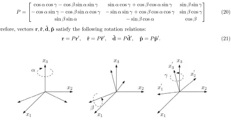
{ˆx₁,xˆ₂,ˆx₃} and {ˆx₁,xˆ₂,xˆ₃}. The system {ˆx₁,xˆ₂,ˆx₃} coincides with the principal directions of the unknown ellipsoid while the system {ˆx₁,xˆ₂,ˆx₃} is a known reference system. In order to specify the orientation and size of the ellipsoid, thex_isystem is transformed tox_isystem with the use of orthogonal rotation matrix P whose elements are given in terms of Euler angles (α, β, γ) (depicted in Figure 2) as follows [11]:

P =

⎡

⎣₋coscosααcossinγγ−−coscosββsinsinααsincosγγ −sinsinααcossinγγ+ cos+ cosββcoscosααsincosγγ sinsinββcossinγγ

sinβsinα −sinβcosα cosβ

⎤

⎦ (20)

Therefore, vectors r,ˆr,dˆ,pˆ satisfy the following rotation relations:

r=Pr, ˆr=Pˆr, dˆ=Pdˆ, ˆp=Pˆp. (21)

Figure 2. Euler angles.

Inserting the rotation relations in Eq. (21) for the directions in the coefficient f(A), they are transformed from the x_i system to x_i. Then by multiplying f(A) with P, we go back to the reference system x_i where the measurements will be taken. The superscript denotes transposition and P=P−1 sinceP is orthogonal. Let

g(A)

ˆr;dˆ,pˆ

:=Pf(A)

Pˆr;Pdˆ, Pˆp

=Pf(A)

ˆr;ˆd,pˆ

. (22)

Therefore

g(A)

ˆ r;ˆd,pˆ

=P

Pˆr×

W(A)Pˆp×Pˆr−T(A)

Pdˆ×Ppˆ

Letting the directions ˆr = εijkxˆk, dˆ = ˆxi and ˆp = ˆxj, where εijk the permutation symbol with εijk=εjki=εkij = 1 andεikj =εjik =εkji =−1, for 1≤i, j, k ≤3 with i, j, k distinct, leads to:

g(A)εijkxˆk; ˆxi,xˆj

=εijkxˆk×

PW(A)Pxˆ_j×εijkxˆk−PT(A)P

ˆ

x_i×xˆ_j, (24) which after calculations can be written as:

g(A)εijkxˆk; ˆxi,xˆj

=

P_i W(A)P_j+εijkPj T(A)Pk

ˆ

x_i+

P_j W(A)P_j −εijkPi T(A)Pk

ˆ

x_j

, (25)

whereP_j =Pxˆ_j is the j-th column of matrixP and P_j = ˆx_jP thej-th row of matrix P. SinceW(A) _{is diagonal for A=I, D, L, the following relations, for 1≤i, j≤3, are obtained:}

P_i W(A)P_j =P_j W(A)P_i. (26)

Taking measurements of the vectors g(I)_,g(D) _{and g}(L)_{, for direction combinations along the axes x} i

and specifically 6 direction combinations which are used to solve for P_i W(A)P_j, leads to: 2P_jW(A)P_j =

g(A)εijkxˆk; ˆxi,xˆj

+g(A)εkjixˆi; ˆxk,xˆj

·xˆ_j, (27) 2P_i W(A)P_j =

2g(A)εijkxˆk; ˆxi,xˆj

−g(A)εjikxˆk; ˆxj,xˆi

+g(A)εkijxˆj; ˆxk,xˆi

·xˆ_i =

2g(A)εjikxˆxk; ˆxj,xˆi

−g(A)εijkxˆk; ˆxi,xˆj

+g(A)εkjixˆi; ˆxk,xˆj

·xˆ_j, (28) The measurement matrices M(A), for the impedance, the lossless and lossy dielectric cases are constructed as follows:

M(A) =

M_ij(A)

, M_ij(A)= 2P_i W(A)P_j (29)

for 1≤i, j≤3. The above relation can be written in matrix form as:

M(A)= 2PW(A)P, (30)

or since the rotation matrixP is orthogonal:

P M(A)P= 2W(A), (31)

which is an orthogonal similarity relation between the measurement matrix M(A) and the diagonal matrixW(A), forA=I, D, L.

The measurement matrixM(A) _{is real and symmetric, and each has three real eigenvaluesλ}(A) n and

three corresponding orthonormal eigenvectors v_n(A) forA=I, D, L. Therefore, based on the orthogonal similarity relation, it is concluded that forn= 1,2,3:

⎧ ⎨ ⎩

λ(nA) = 2Wn(A),

v_n =

P_n(A1), P (A) n2 , P

(A) n3

, (32)

where P_n(A1), P (A) n2 , P

(A)

n3 are elements of the nth row of rotation matrix P, and the superscript A

denotes the case of the impedance (I), lossless dielectric ellipsoid (D) and lossy dielectric ellipsoid (L), respectively. From elements of the three orthogonal eigenvectors in each case, the elements of matrixP are obtained, and therefore the Euler angles are specified by using the following relations [11]:

α(A)= sin−1

⎛

⎝ P31(A)

1−P332(A)

⎞

⎠_{, β}(A)_{= sin}−1

1−P332(A) , γ

(A)_{= sin}−1

⎛

⎝ P13(A)

1−P332(A)

⎞

⎠_. (33)

From the system of equations that connect the eigenvalues with the elements of the diagonal matrices W(I), W(D), W(L), the following system of equations forn= 1,2,3 is obtained:

λ(_nI) = 2 3

1

I1n

, (34)

λ(_nD) = 2V

(D)

3

μ+η2−μ−

(μ+_η2−_μ−_)V(D)_In 1 +μ−

, (35)

λ(_nL) = 2 3

1

I1n

. (36)

From these equations, the semi-axes α1, α2, α3 are specified, and therefore, the size of the impedance,

lossless and lossy dielectric ellipsoids is obtained. Specifically, improper elliptic integrals are specified directly from the eigenvalues via the following relations:

I1n =

2

3λ(nI)

, (37)

I1n =

2

3λ(nD) − 2μ

−_λ(D) 1 λ

(D) 2 +λ

(D) 2 λ

(D) 3 +λ

(D) 1 λ

(D) 3

3 (μ+_η2_{+ 2μ}−_)λ(D) 1 λ

(D) 2 λ

(D) 3

. (38)

I1n =

2

3λ(nL)

. (39)

Moreover, the quantitiesV(A)can also be found in terms of the eigenvalues using the relation in Eq. (15). Having found the quantitiesI1n forn= 1,2,3 and using the relations that connect the improper elliptic

integrals with the incomplete elliptic integrals of the first kind (F) and the second kind (E) ([11], p. 381):

I11 =

1

h2h23

(F(φ, α)−E(φ, α)), (40)

I12 =

h2

(h22−h23)h23

E(φ, α)− 1

h2h23

F(φ, α)− 1 (h22−h23)

α21−h22 α1

α21−h23

, (41)

I13 = −

1 (h22−h23)h2

E(φ, α) + 1 (h22−h23)

α2 1−h23 α1

α21−h22

, (42)

leads to a system of three equations for the three unknownsα1, h2, h3 which can be solved using various

softwares (e.g., Matlab), and the three semi-axes can be obtained via the relations α2 =

α21−h23 and α3 =

α21−h22. Alternatively, one can proceed similar to the method described in [9].

Note here that the inverse problem can also be solved using directions of observation in the forward and backward directions of propagation instead of the directions of magnetic polarization as in the method described above. In this case, letting ˆr = cxˆ_i (with c = ±1), ˆd = ˆx_i and ˆp = ˆx_j for 1≤i, j≤3, leads to:

g(A)cxˆ_i; ˆx_i,xˆ_j =

P_j W(A)P_j +cP_kT(A)P_k

ˆ

x_j+

P_kW(A)P_j−cP_jT(A)P_k

ˆ

x_k

, (43)

for A=I, D, L. Taking measurements for direction combinations similar to the previous method and solving forP_kW(A)_P

j leads to:

2P_jW(A)P_j =

g(A)ˆx_i; ˆx_i,xˆ_j+g(A)−xˆ_i; ˆx_i,ˆx_j·xˆ_j (44) 2P_kW(A)P_j =

g(A)ˆx_i; ˆx_i,xˆ_j+g(A)−xˆ_i; ˆx_i,ˆx_j·xˆ_k =

g(A)ˆx_i; ˆx_i,xˆ_k+g(A)−xˆ_i; ˆx_i,ˆx_k·xˆ_j (45) Therefore, the following matrix is constructed:

4. GEOMETRICALLY DEGENERATE FORMS

The cases of spheroids and spheres can be considered as geometrically degenerate forms of the ellipsoid. Specifically, for the sphere, the following relations are valid:

α1 =α2=α3, h2 =h3 =μ=ν = 0, I1n(ρ) =

1

3ρ3, (47)

forn= 1,2,3.

For the case of spheroids, the following relations are valid:

prolate spheroid: α1> α2 =α3, h2=h3, (48)

oblate spheroid: α1 =α2> α3, h3 = 0. (49)

Based on the relation:

I1i−I1j =

α2_j −α2_i

2

_∞

0

dx

(x+α2_i)(x+α2_j)R(x), (50)

withR(x) =(x+α21)(x+α22)(x+α23), it can be observed that whenλ1 =λ2 =λ3⇒ α1 =α2 =α3

which means that the unknown scatterer is a sphere independent of orientation and radiusα1 =V 1 3. In the case that two out of the three eigenvalues are equal, i.e.,λ2=λ3, the scatterer is a spheroid.

Thus, based on [9] and the fact that M2=M3, the following equation is valid:

1

1−

α1 α2

2

⎡ ⎢ ⎢ ⎢ ⎢ ⎣1−

α1 α2

cos−1

α1 α2

1−

α1 α2

2

⎤ ⎥ ⎥ ⎥ ⎥

⎦=M1, (51)

and the semi-axes are given by:

α1 =

α21 α22

V 1 3

, α2=α3 =

V α2 α1

1 3

, (52)

where V can be found in terms of eigenvalues λ1 and λ2 =λ3 using identity (15) since I1n can also be

found in terms of them via relations in Eqs. (37)–(39) for each case, respectively.

5. NUMERICAL RESULTS

In this section, numerical results following this method are presented:

Numerical example

Taking far-field measurements and following the numerical algorithm depicted in the flowchart given in the Appendix, the corresponding measurement matrix is constructed, and based on its eigenvalues and eigenvectors the following numerical example is presented:

For measurements that give the measurement matrix:

M =

₉₆

.1185 −0.4228 17.8598

−0.4228 88.0748 −0.3351 17.8598 −0.3351 87.7339

,

with eigenvalues and eigenvectors:

λ1 = 110.2845, λ2= 88.0617, λ3= 73.5810,

v1 = (0.7835,−0.0243,0.6209), v2= (−0.0190,−0.9997,−0.0151), v3 = (−0.6211,0.0000,0.7837),

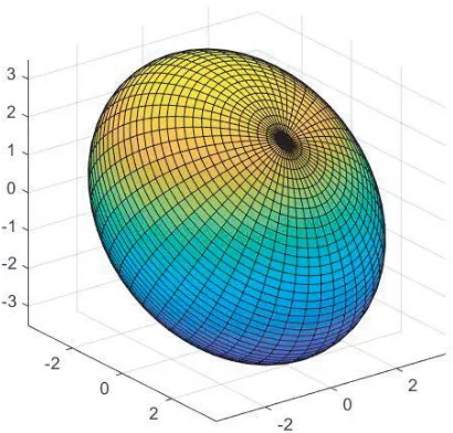
the following results are obtained which are depicted in Figure 3.

Where the Euler angles areα=−1.5708,β = 0.6701,γ = 1.5465 and its semi-axes areα1 = 4.2002, α2 = 3.5004 andα3= 2.9962.

Figure 3. Reconstruction of an ellipsoid using far-field data.

6. CONCLUSION

In the preceding work, the theoretical results concerning a method for solving an inverse electromagnetic scattering problem for the cases of an impedance or a dielectric ellipsoid are presented. In particular, using six measurements of the leading order low-frequency coefficient of the electric far-field pattern, a measurement matrix is constructed whose eigenvalues and eigenvectors are used to specify the size and orientation of the unknown ellipsoid, respectively. Finally, a numerical example is presented. Therefore, the presented method can lead to an efficient algorithm.

REFERENCES

1. Athanasiadis, C., P. Martin, and I. G. Stratis, “On spherical-wave scattering by a spherical scatterer and related near-field inverse problems,”IMA J. Appl. Math., Vol. 66, 539–549, 2001.

2. Athanasiadis, C.,Wave Propagation Elements and Applications, HOU, Patras, Greece, 2015. 3. Athanasiadis, C. and N. Tsitsas, “Point-source excitation of a layered sphere: Direct and far-field

inverse scattering problems,” Quarterly Journal of Mechanics and Applied Mathematics, Vol. 61, 549–580, 2008.

4. Apostolopoulos, T., K. Kiriaki, and D. Polyzos, “The inverse scattering problem for a rigid ellipsoid in linear elasticity,” Inverse Problems, Vol. 6, 1–9, 1990.

5. Colton, D. and R. Kress,Inverse Acoustic and Electromagnetic Scattering Theory, 2nd Edition, ed. Springer, Berlin Heidelberg, 1998.

6. Dassios, G., “The inverse scattering problem for the soft ellipsoid,” Journal of Mathematical Physics, Vol. 28, 2858–2862, 1987.

7. Dassios, G. and K. Kiriaki, “Size, orientation, and thickness identification of an ellipsoidal shell,”

Workshop on Inverse Problems and Imaging, Glasgow 1989, Proceedings, 38–48, Glasgow, 1991. 8. Dassios, G. and R. Lucas, “Inverse scattering for the penetrable ellipsoid and ellipsoidal boss,”

Journal of the Acoustical Society of America, Vol. 99, 1877–1882, 1996.

9. Dassios, G. and R. Lucas, “Electromagnetic imaging of ellipsoids and ellipsoidal bosses,”Quarterly Journal of Mechanics and Applied Mathematics, Vol. 51, 413–426, 1998.

10. Dassios, G. and R. Kleinman,Low Frequency Scattering, Oxford University Press, Oxford, 2000. 11. Dassios, G., Ellipsoidal Harmonics: Theory and Applications, Cambridge University Press,

Cambridge, 2012.

12. Lucas, R. J., “An inverse problem in low-frequency scattering by a rigid ellipsoid,”Journal of the Acoustical Society of America, Vol. 95, 2330–2333, 1994.

13. Shifrin, E. I. and P. S. Shushpannikov, “Reconstruction of an ellipsoidal defect in anisotropic elastic solid, using results of one static test,”Inverse Problems in Science and Engineering, Vol. 21, 781–800, 2013.