Off-Grid Direction-of-Arrival Estimation Using a Sparse Array
Covariance Matrix
Xiaoyu Luo*, Xiaochao Fei, Lu Gan, and Ping Wei
Abstract—An off-grid direction-of-arrival (DOA) estimation method that utilizes a sparse array covariance matrix is proposed. In this method, the array covariance matrix is sparsely represented in the form of a vector and then modified to become an off-grid DOA estimation model according to the first-order Taylor series. By solving for the two sparse vectors in the resulting array covariance matrix, the off-grid DOA estimation can thus be achieved. We present an alternating iterative algorithm that exploits the alternating update of a convex optimization problem and a least-squares problem to solve for these two sparse vectors. Our method also extends the aperture. The effectiveness and efficiency of the proposed method are demonstrated in the simulation results.
1. INTRODUCTION
Direction-of-arrival (DOA) estimation is of great importance in applications of radar, sonar, and communication [1]. In this respect, many subspace-based methods as represented by multiple signal classification (MUSIC) [2] have been proposed to estimate directions of arrival (DoAs). When signals are uncorrelated and the number of snapshots is large, the MUSIC method is proven to be equivalent to the maximum likelihood (ML) method [3].
In recent years, the exploration of the sparsity of signals facilitates the progress of DOA estimation and a variety of sparse representation-based methods [4–8] have been advanced to estimate DoAs. 1 -SVD [4] and sparse covariance-based estimation (SPICE) [5] are prevalent ones. The former exploits the 1 norm to reconstruct sparse signals and applies singular value decomposition (SVD) to reduce computational complexity and noises, whereas the latter employs the array covariance matrix to improve its accuracy. Nevertheless, in these sparse representation-based methods the true values of all DoAs are assumed to be located on a selected sampling grid. When the assumption fails, the performance of such methods deteriorates due to the problem of mismatch. Accordingly, several methods have been raised to study the off-grid DOA estimation (i.e., estimating DoAs under the circumstance that the true values of all or some DoAs are out of the selected sampling grid), and they are built upon the principle of sparse signal reconstruction in the presence of the off-grid problem introduced in [9]. The authors of [10] present an off-grid model and put forward the sparse total least-squares (STLS) method. However, this model is not appropriate for the off-grid DOA estimation. The performance of the STLS method is thus poor in this sense. Mixed norm-based methods are then proposed to estimate off-grid DoAs in [11–13]. These methods still perform unsatisfactorily since they require the reconstruction of a sparse matrix rather than a sparse vector. In [12], the authors also advance the joint orthogonal matching pursuit (J-OMP) method, but the performance of J-OMP relies on the number of sensors. The methods in [14, 15] utilize off-grid sparse Bayesian inference (OGSBI) to estimate off-grid DoAs. Yet, the drawback of them is that their performance is sensitive to initial parameters. The method
Received 3 March 2015, Accepted 11 June 2015, Scheduled 23 June 2015
* Corresponding author: Xiaoyu Luo ([email protected]).
developed in [16] poses a block sparse estimator for the off-grid DOA estimation. Since the estimator works only with a single snapshot, its accuracy is low.
In this paper, we attempt to obtain the off-grid DOA estimation using a sparse array covariance matrix, so the method proposed here is referred to as off-grid sparse array covariance matrix (OGSACM). The OGSACM method converts the array covariance matrix into a vector and then sparsely represents the resulting vector in an over-complete Kronecker basis. Afterwards, the sparse array covariance matrix is turned into an off-grid DOA estimation model by means of the first-order Taylor series. Finally, an alternating iterative algorithm that utilizes the alternating update of a convex optimization problem and a least-squares (LS) problem is presented to solve for the two sparse vectors in the modified sparse array covariance matrix and the off-grid DOA estimation is then achieved. The reason for employing the alternating iterative algorithm is concluded in [17] that a single 1-norm minimization cannot deal with this solution. Our OGSACM method overcomes the aforementioned drawbacks of the state-of-the-art methods. Moreover, in OGSACM the vector resulting from the transformation of array covariance matrix extends the aperture. The simulation results show that the OGSACM method is valid and performs better than the state-of-the-art methods in the off-grid DOA estimation.
Nomenclature: The superscripts T, H, ∗, −1, and † denote the transpose, conjugate transpose, conjugate, inverse and pseudo inverse, respectively. The notationsE[·], vec(·),IM,⊗, diag(·), · P, and
| · |represent the mathematical expectation, vectorization,M×M identity matrix, Kronecker product, diagonal matrix,p norm, and absolute value, respectively.
2. OFF-GRID MODEL
Consider a uniform linear array (ULA) with M isotropic sensors and inter-element spacingdas shown in Figure 1. Suppose thatK uncorrelated far-field narrowband signals of wavelength λimpinge on this ULA from distinct directions [θ1, θ2, . . . , θK].
The received signalsxat time tcan then be written as
x(t) =A(θ)s(t) +n(t). (1) The matrices and vectors in (1) take the following forms:
x(t) = [x1(t), x2(t), . . . , xM(t)]T ∈CM×1,
A(θ) = [a(θ1),a(θ2), . . . ,a(θK)]∈CM×K,
a(θk) =
1, e−jϕk, . . . , e−j(M−1)ϕkT, ϕ
k= 2πd
λ sinθk,
s(t) = [s1(t), s2(t), . . . , sK(t)]T ∈CK×1,
n(t) = [n1(t), n2(t), . . . , nM(t)]T ∈CM×1,
(2)
where A(θ) represents the array flow pattern, a(θk) the steering vector, s(t) the incident signals, and
n(t) the additive Gaussian white noise vector with the mean and variance of each element equal to zero and σ2 respectively. The array covariance matrix R of the received signals can thus be derived by
R=Ex(t)xH(t)=A(θ)RsAH(θ) +σ2IM, (3) where Rs = diag(r1, r2, . . . , rK) with ri, i= 1,2, . . . , K being the power of incident signals. We then convert the array covariance matrixR into a vector r, which yields
r= vec (R) =G(θ)rs+σ2vec (IM), (4)
whereG(θ) = [g(θ1),g(θ2), . . . ,g(θK)]∈CM
2×K
and rs= [r1, r2, . . . , rK]T with
g(θk) = vec
a(θk)aH(θk)
=a∗(θk)⊗a(θk), k= 1,2, . . . , K (5)
We further have
a∗(θk)⊗a(θk) =
aT (θk), ejϕkaT(θk), . . . , ej(M−1)ϕkaT (θk) T
(6)
From (2) and (6), it can be seen that the number of different entries in g(θk) is greater thanM, so the aperture is extended. The sparse representation of ris thus given by
r=G(˜θ)˜rs+σ2vec (IM), (7)
where ˜θ= [˜θ1,θ˜2, . . . ,θN˜ ] is the selected sampling grid ranging from−90◦to 90◦, and˜rs=[˜r1,r˜2, . . . ,rN˜ ] is the K-sparse vector withr1, r2, . . . , rK being its K nonzero elements.
Note that solving for˜rs we can get [θ1, θ2, . . . , θK] if and only if G(θ) ∈G(˜θ). However, the case
G(θ) ∈/ G(˜θ) is more common and the performance of DOA estimation deteriorates in the presence of such case. Therefore, we modify the sparse representation of rin (7).
We first expand g(θk),k= 1,2, . . . , K by the first-order Taylor series, namely,
g(θk)≈g
˜
θsk +h
˜ θsk
˜
θsk−θk , (8)
where |θs˜k −θk| = min{|θ˜1−θk|,|θ˜2−θk|, . . . ,|θN˜ −θk|} and h(˜θsk) = d
g(˜θsk)
dθ˜sk . Since there is correspondence between θ and sinθ when θ ranges from −90◦ to 90◦, θ can be substituted by sinθ. (8) is then rewritten as
g(sinθk)≈g
sin ˜θsk +h
sin ˜θsk βk, (9)
whereβk= sin ˜θsk−sinθk. By (9), the calculation is simplified. Accordingly, (4) becomes
r=
G
sin ˜θs +H
sin ˜θs diag (β)
rs+σ2vec (IM) =G
sin ˜θs rs+H
sin ˜θs diag(rs)β+σ2vec(IM) (10)
where ˜θs= [˜θs1,θs˜2, . . . ,θs˜K] andβ= [β1, β2,. . . , βK]T. The sparse representation ofris thus modified as
r=G
sin ˜θ ˜rs+H
sin ˜θ diag (˜rs)β˜+σ2vec (IM), (11)
whereβ˜∈CN×1 is the K-sparse vector withβ1, β2, . . . , βK being its K nonzero elements.
3. OFF-GRID DOA ESTIMATION
From (11) and [17], we can solve for˜rs and β˜by minimizing the 1 norm. It is then immediate that
˜rs,β˜ = arg min ˜ ri0,β˜
˜rs1+δr−σ2vec (IM)−G(sin ˜θ)˜rs−H(sin ˜θ)diag (˜rs)β˜
2 (12)
where ˜ri is the ith element of ˜rs. Nevertheless, the above optimization problem is nonconvex [17]. Consequently, the following alternating iterative algorithm is presented to solve respectively for˜rs and
˜
β, that is,
˜r(sj)= arg min ˜
ri0˜rs1+δ
r−σ2vec (IM)−G(sin ˜θ)˜rs−H(sin ˜θ)diag (˜rs)β˜(j−1)
2 (13)
and
β(j)= arg min β
r−σ2vec (IM)−G(j)(sin ˜θs)r(sj) −H(j)(sin ˜θs)diag
r(sj) β
2 (14)
where j denotes the jth iteration and δ is a parameter generally set to be 0.5 [18, 19]. σ2 is estimated
by M−1KM−K i=1
In the jth iteration, G(j)(sin ˜θs) and H(j)(sin ˜θs) in (14) are formed respectively by the vectors of
G(sin ˜θ) and H(sin ˜θ) located according to the indices of the K peaks of ˜r(sj) and the elements of r(sj)
in (14) take on the same values as the K peaks of˜rs(j). In the (j+ 1)th iteration, β(j) is extended to become an N×1 vector β˜(j) whose K elements located by the indices of the K peaks of˜r(j)
s have the same values as the elements of β(j) and remainingN −K elements equal zero.
The iteration starts with β˜(0) = 0N×1, where 0N×1 = [0,0, . . . ,0]T ∈ CN×1 and proceeds until
|˜r(sj+1)1−˜r(sj)1|
˜r(sj)1 e
, where e is a threshold set to be 10−4. Since β˜(0) =0N×1 is constant and implies
that no true values of DoAs are off grid, the iteration is not affected by initial parameters.
In (14), sinceH(j)(sin ˜θs) and diag(r(sj)) are the column full-rank and full-rank matrices respectively, there is a unique LS solution to β(j). We can then solve forβ(j) by
β(j)=
diag
r(sj) −1
H(j)
sin ˜θs
†
r−σ2vec (IM)−G(j)
sin ˜θs r(sj)
(15)
The optimal solution (˜rs,β˜) is thus obtained by the alternating update of (13) and (15). Following the proof in [17], we can easily show that (˜rs,β˜) is also the optimal solution of (12).
Assume that the number of iterations is m and the indices of the K peaks of ˜r(sm) are [s(1m), s
(m) 2 , . . . , s
(m)
K ] respectively. The off-grid DOA estimation of the kth signal is thus achieved by
θK = arcsin
sin ˜θs(m)
k −β
(m)
k , k= 1,2, . . . , K, (16)
whereβ(km) is thekth element of β(m).
4. SIMULATION
Numerical examples are presented to test the validity of the OGSACM method and compare the accuracy of OGSACM, OGSBI [12], sparse spectral fitting with modeling uncertainty (SSFMU) [8], and 1 -SVD [4] in the off-grid DOA estimation. In the simulation, M = 8 isotropic sensors with inter-element spacing d = λ/2 are assumed to be on the ULA. There are two uncorrelated far-field narrowband signals impinging on this ULA from directions −14.5◦ and 36.3◦ respectively. A uniform sampling grid [−90◦,−90◦+ Δ, . . . ,90◦−Δ,90◦] is selected, where Δ denotes the grid interval. We define the input signal-to-noise ratio (SNR) as 10 lg(γs/σ2), where γs is the total power of signals andσ2 is the power of noise.
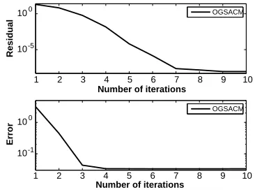
In the first numerical example, we illustrate the effectiveness of the OGSACM method. The measure adopted here is the residual and error of˜rs defined respectively as
Residual =˜r(sj+1)−˜r(sj)
1 (17)
and
Error =˜r(sj)−˜rtrues
1, (18)
where˜rtrues is the true value of˜rs. In this numerical example, Δ = 2◦. In addition, the SNR is 10dB and the number of snapshots is 250.
Figure 2 depicts the changes in the residual and error of ˜rs with the increase in the number of iterations. It is observed that both the residual and the error get closer to zero as the number of iterations goes from 1 to 10. These results indicate that ˜rs converges to its true counterpart as the number of iterations increases. The same is true for β˜ according to (15). Therefore, our OGSACM method is valid.
In the second numerical example, we compare the estimated accuracy of OGSACM with that of OGSBI, SSFMU, and1-SVD. The measure is the root mean square error (RMSE) defined as
RMSE = 1
L 1 K
L
i=1 K
k=1
θk−θˆ(ki) 2
1 2 3 4 5 6 7 8 9 10 10
10
Number of iterations
Residual
1 2 3 4 5 6 7 8 9 10
10 10
Number of iterations
Error
OGSACM
OGSACM -5
0
-1 0
Figure 2. The residual and error versus the number of iterations.
-4 0 5 10 15 20
10 10 10 10
SNR (dB)
RMSE (deg)
OGSACM OGSBI SSFMU L1 SVD CRLB
-2 -1 0 1
Figure 3. The RMSE versus the SNR.
100 150 200 250 300 350 400
10 10 10 10
Number of snapshots
RMSE (deg)
OGSACM OGSBI SSFMU L1 SVD CRLB
-2 -1 0 1
Figure 4. The RMSE versus the number of snapshots.
1 1.5 2 2.5 3 3.5 4
10 10 10 10
Grid interval (deg)
RMSE (deg)
OGSACM OGSBI SSFMU L1 SVD
-2 -1 0 1
Figure 5. The RMSE versus the grid interval.
where L= 500 is the number of times of Monte Carlo experiments and ˆθ(ki) the estimated angle of the Kth signal in the ith experiment.
We plot the RMSEs for OGSACM, OGSBI, SSFMU, and1-SVD under three different conditions in Figures 3, 4, and 5 respectively. The Cramer-Rao lower bound (CRLB) [3] also appears in Figures 3 and 4. In Figure 3, the SNR ranges from−4 dB to 20 dB and the number of snapshots is fixed at 250. In Figure 4, the number of snapshots ranges from 100 to 400 and the SNR is fixed at 10 dB. In both Figures 3 and 4, Δ = 2◦. In Figure 5, Δ ranges from 1◦to 4◦, and the SNR and the number of snapshots are fixed at 10dB and 250 respectively.
As displayed in Figures 3, 4, and 5, there exist sustained error in 1-SVD, suggesting that this method cannot estimate off-grid DoAs. This is because it is assumed in its DOA estimation model that the true values of all DoAs are located on the selected sampling grid. Figures 3, 4, and 5 also reveal that the accuracy of OGSACM is higher than that of OGSBI and SSFMU. The reason for outperforming the OGSBI method is that the performance of OGSACM is unaffected by initial parameters while the performance of OGSBI is vulnerable to its initial random vector (e.g., the OGSBI method performs poorly when the value of the initial random vector is far different from its true counterpart), and the reason for performing better than SSFMU is that OGSACM requires the reconstruction of merely a sparse vector whereas SSFMU a sparse matrix. Furthermore, the extended aperture also makes the OGSACM method more accurate.
5. CONCLUSION
1-norm minimization is not capable of doing so. Besides, the aperture is extended in this method. Both the alternating iterative algorithm and the extended aperture lead to an improvement in the performance of OGSACM. As shown in the simulation results, our OGSACM method is effective and performs better than the state-of-the-art methods.
REFERENCES
1. Krim, H. and M. Viberg, “Two decades of array signal processing research: The parametric approach,”IEEE Trans. Signal Process. Mag., Vol. 13, No. 4, 67–94, 1996.
2. Schmidt, R., “Multiple emitter location and signal parameter estimation,” IEEE Trans. Antennas Propag., Vol. 34, No. 3, 276–280, 1989.
3. Stoica, P. and A. Nehorai, “MUSIC, maximum likelihood, and Cramer-Rao bound,”IEEE Trans. Acoust., Lett., Vol. 34, No. 3, 276–280, 1986.
4. Malioutov, D., M. Cetin, and A. S. Willsky, “A sparse signal reconstruction perspective for source localization with sensor arrays,”IEEE Trans. Signal Process., Vol. 53, No. 8, 3010–3022, 2005. 5. Stoica, P., P. Babu, and J. Li, “SPICE: A sparse covariance-based estimation method for array
processing,” IEEE Trans. Signal Process., Vol. 59, No. 2, 629–638, 2011.
6. Yin, J.-H. and T.-Q. Chen, “Direction-of-arrival estimation using a sparse representation of array covariance vectors,”IEEE Trans. Signal Process., Vol. 59, No. 9, 4489–4493, 2011.
7. He, Z.-Q., Q.-H. Liu, L.-N. Jin, and S. Ouyang, “Low complexity method for DOA estimation using array covariance matrix sparse representation,”Electronics Letters, Vol. 49, No. 3, 228–230, 2013. 8. Carlin, M., P. Rocca, G. Oliveri, F. Viani, and A. Massa, “Directions-of-arrival estimation through bayesian compressive sensing strategies,”IEEE Trans. Antennas Propag., Vol. 61, No. 7, 3828–3838, 2013.
9. Tang, G., B. N. Bhaskar, P. Shah, and B. Recht, “Compressed sensing off the grid,” IEEE Trans. Inf. Theory, Vol. 59, No. 11, 7465–7490, 2013.
10. Zhu, H., G. Leus, and G. Giannakis, “Sparsity-cognizant total least-squares for perturbed compressive sampling,”IEEE Trans. Signal Process., Vol. 59, No. 5, 2002–2016, 2011.
11. Zheng, J.-M. and M. Kaveh, “Directions-of-arrival estimation using a sparse spatial spectrum model with uncertainty,”IEEE Int. Conf. Acoustics, Speech and Signal Processing (ICASSP), 2848–2851, 2011.
12. Tan, Z. and A. Nehorai, “Sparse direction of arrival estimation using co-prime arrays with off-grid targets,”IEEE Trans. Signal Process. Lett., Vol. 21, No. 1, 26–29, 2014.
13. Tan, Z., P. Yang, and A. Nehorai, “Joint sparse recovery method for compressed sensing with structured dictionary mismatches,”IEEE Trans. Signal Process., Vol. 62, No. 19, 4997–5008, 2014. 14. Yang, Z., L.-H. Xie, and C.-S. Zhang, “Off-grid direction of arrival estimation using sparse Bayesian
inference,”IEEE Trans. Signal Process., Vol. 61, No. 1, 38–43, 2013.
15. Zhang, Y., Z.-F. Ye, X. Xu, and N. Hu, “Off-grid DOA estimation using array covariance matrix and block-sparse Bayesian learning,”Signal Process., Vol. 98, 197–201, 2014.
16. Jagannath, R. and K. V. S. Hari, “Block sparse estimator for grid matching in single snapshot DoA estimation,” IEEE Trans. Signal Process. Lett., Vol. 20, No. 11, 1038–1041, 2013.
17. Yang, Z., C.-S. Zhang, and L.-H. Xie, “Robustly stable signal recovery in compressed sensing with structured matrix perturbation,”IEEE Trans. Signal Process., Vol. 60, No. 9, 4658–4671, 2012. 18. Donoho, D. L., M. Elad, and V. N. Temlyakov, “Stable recovery of sparse overcomplete
representations in the Presence of Noise,” IEEE Trans. Inf. Theory, Vol. 52, No. 1, 6–18, 2006. 19. Tropp, J. A., “Just relax: Convex programming methods for identifying sparse signals in noise,”