Fast Schemes for Computing Similarities between
Gaussian HMMs and Their Applications in Texture
Image Classification
Ling Chen
Department of Electrical and Computer Engineering, Stevens Institute of Technology, Castle Point on Hudson, Hoboken, NJ 07030, USA
Email:[email protected]
Hong Man
Department of Electrical and Computer Engineering, Stevens Institute of Technology, Castle Point on Hudson, Hoboken, NJ 07030, USA
Email:[email protected]
Received 31 December 2003; Revised 18 August 2004
An appropriate definition and efficient computation of similarity (or distance) measures between two stochastic models are of theoretical and practical interest. In this work, a similarity measure, that is, a modified “generalized probability product kernel,” of Gaussian hidden Markov models is introduced. Two efficient schemes for computing this similarity measure are presented. The first scheme adopts a forward procedure analogous to the approach commonly used in probability evaluation of observation sequences on HMMs. The second scheme is based on the specially defined similarity transition matrix of two Gaussian hidden Markov models. Two scaling procedures are also proposed to solve the out-of-precision problem in the implementation. The effectiveness of the proposed methods has been evaluated on simulated observations with predefined model parameters, and on natural texture images. Promising experimental results have been observed.
Keywords and phrases:similarity measure, hidden Markov model, kernel method, Bhattacharyya affinity, texture classification.
1. INTRODUCTION
Hidden Markov model(HMM) has been adopted in a wide variety of application areas including econometrics, compu-tational biology, statistical process control, and speech recog-nition. Recently, it was also introduced to image processing applications such as face recognition [1,2] and texture analy-sis [3,4]. A challenging problem for HMM is that given their model parameters, how to define an appropriate similarity (or distance) measure for two HMMs [5].
An appropriate similarity measure between two HMMs is of theoretical interests and it can also be a useful tool in various applications. For instance, in computational biology, because of the availability of large libraries of profile HMMs, there exists the possibility of comparing sequence families by comparing the profiles of the families rather than comparing the individual members of the families. It is also possible to compare a sequence family instead of its individual members towards an HMM that is trained to model a particular feature [6]. In image retrieval applications, each texture image can be modeled by a wavelet-domain HMM and the classification is
carried out by computing distances between the model of the query image and those of all candidate images [4].
There have been some research efforts on this prob-lem and several techniques are proposed in the literature [4,5,6,7,8]. To begin with, denoteλ = (A,B,π) as the model parameters of an HMM, whereAis astate transition distribution,Bis theobservation probability distribution, and
πis theinitial state distribution. DenoteX=(x1,x2,. . .,xT) as an observation sequence generated byλ. Observationsx can be either discrete symbols chosen from a finite alphabet (x ∈ V = {v1,v2,. . .,vM}) or continuous (vector) signals (x∈ND). In [5], a distance measure between two HMMs,λ andλ, was proposed as
D(λ,λ)= 1
T
logP(X|λ)−logP(X|λ), (1) whereXis an observation sequence generated by the model
λ. A symmetrized version of this distance measure is
Ds(λ,λ)=D
(λ,λ) +D(λ,λ)
In [6], thecoemission probabilityof two profile HMMs is de-fined as
X∈V×···×V
P(X|λ)P(X|λ), (3)
whereλandλare two profile HMMs. In [4], the distance be-tween the two HMMs is computed based on Kullback-Leibler (KL) distance:
D(λ,λ)=
ND×···×NDP(X|λ) log
P(X|λ)
P(X|λ)dX. (4) Recently, ageneralized probability product kernel(GPPK) be-tween distributions, which represents the similarity bebe-tween two probability distributionspandp, is proposed [8]:
Kρ(p,p)=
Ωp(x)
ρp(x)ρdx, (5)
where normally ρ ∈ {1/2, 1, 2, 3,. . .}. The motivation be-hind this method is to combine discriminative and genera-tive estimations to exploit their complementary advantages. In [8], theexpected likelihood kernel, that is,K1(p,p), is used
to derive the similarity measure between Gaussian mixture models, HMMs, and so forth. Some of the advantages of the GPPK include the positive-definite, symmetric property and the capability to handle a variety of generative models (in-cluding HMMs) in a closed form (note that KL distance is not positive definite, asymmetric and in many cases, it can only be approximated by an upper bound). However, the closed-form evaluation of GPPK is not readily available ex-cept for ρ = 1. Whereas other values of ρ, especiallyρ =
1/2, can also be of great interest in some cases, notice that whenρ=1/2, the GPPK is effectively the well-known
Bhat-tacharyya’s measure of affinity between two statistical distri-butions [9]. In this work, we develop a modified GPPK to efficiently evaluate similarity between HMMs in closed form whereas the value ofρcan be chosen freely, that is, not con-strained to 1. The modification is developed based on a new interpretation of GPPK. Under this new interpretation, the similarity measure of two HMMs is considered as the sta-tistical average of similarities of all possible so-calledcostate sequencesdrawn from the two HMMs.
Meanwhile, the brute-force computation of the simi-larity between two Gaussian HMMs can be prohibitively intensive, for example, the computational complexity is
O(3T(NN)T+1), whereT is the number of transitions and
N andN are the numbers of states of two HMMs. In this work, we propose two fast schemes which can drastically ease this burden by reducing the computational complexity to
O(3T(NN)2) andO((NN)3log
2T), respectively. The
rela-tive computational complexity of these two schemes depends on the complexities of the two HMMs, for example, the num-ber of statesN and the number of transitionsT to be used in the evaluation process. It can be measured by the ratio of 3T/NNlog2T.
Another important implementation issue of the pro-posed similarity measure is the out-of-precision problem.
Because the computation of similarity between HMMs will exceed the precision limit of any machines whenTgets large, we formulate two scaling procedures corresponding to two proposed fast schemes. The scaling procedures can prevent the computation from going beyond the precision range as well as guarantee that the exact value of the similarity mea-sure can be evaluated.
The paper is arranged as follows.Section 2 introduces the similarity measure of Gaussian HMMs and its modifica-tion.Section 3presents the forward procedure and its scaling procedure for computing the proposed similarity measure.
Section 4presents the second fast scheme based on similarity transition matrix, which is followed by the scaling procedure.
Section 5provides the preliminary experimental results. We conclude our work inSection 6.
2. SIMILARITY MEASURE OF GAUSSIAN HMMS
AND ITS MODIFICATION
One of the building blocks in deriving the similarity measure of general HMMs is computing the similarity measure of any arbitrary pair of observation distributions corresponding to two specific states of these two HMMs, denoted asψs,s. For Gaussian HMMs, the observation probability distribution is Gaussian. Based on (5), the GPPK of two D-dimensional Gaussians, p(x)∼N(µ,Σ) andp(x)∼N(µ,Σ), is com-puted as
ψN,N=Kρ(p,p)
=
RDp(x)
ρp(x)ρdx
=(2π)(1−2ρ)D/2|Σ†|1/2|Σ|−ρ/2|Σ|−ρ/2
×exp
−ρ
2µ
TΣ−1µ−ρ
2µ TΣ−1µ
+1 2µ
†TΣ†µ†,
(6)
whereΣ† = (ρΣ−1+ρΣ−1)−1andµ† = ρΣ−1µ+
ρΣ−1µ. Note that the computational complexity ofψN,N is mainly determined by the complexity of matrix determinants and inverses (which both areO(D3)) in (6).
For Gaussian HMM, given the observation sequenceX and the model parametersλ, the likelihood is
P(X|λ)=
N
s0,...,sT=1
πs0b
x0|s0
T
t=1
bxt|st
ast|st−1, (7)
where πs0 is the initial state probability of states0,b(xt|st) is the Gaussian distribution corresponding to state st, and
ast|st−1 is the state transition probability from statest−1tost. Whenρ=1, the GPPK of two Gaussian HMMs is
Kρ(λ,λ)
=
RD×···×RDP(X|λ)P(X|λ )dX
=
N
s0,...,sT=1 N
s0,...,sT=1
πs0πs0ψs0,s0 T
t=1
whereψst,st,t =0, 1, 2,. . .,T, is the GPPK of two Gaussians corresponding to statesstandstof two HMMs.1
The derivation of (8) is based on the definition of GPPK with the value ofρbeing set to 1. Here we take another per-spective to derive the similarity measure that is exactly the same as the one depicted in (8), whereas the value of ρis no longer constrained to be 1. For two HMMs λ andλ, suppose from t = 0 to t = T that the state sequence is s=(s0,s1,s2,. . .,sT) ands=(s0,s1,s2,. . .,sT). Then we de-fine a “costate” sequence asss=(s0,s0,s1,s1,. . .,sT,sT). The probability of such a costate sequencesswith model param-etersλandλcan be computed as
P(ss|λ,λ)=P(s|λ)P(s|λ)=πs0πs0 T
t=1
ast|st−1ast|st−1. (9)
Define the similarity of two state sequences as
ψss= T
t=0
ψst,st. (10)
The value of ψss is determined by the value of ρ used in the computation of ψst,st, that is, the GPPK of two Gaus-sians corresponding to two statesst andst of two Gaussian HMMs (see (6)). Then the similarity measure betweenλand
λ, given an arbitrary costate sequencess, is the product of the probability of the costate sequence and the correspond-ing similarity of the two state sequences, that is,
Kρ∗(λ,λ|ss)=P(ss|λ,λ)ψss
=πs0πs0 T
t=1
ast|st−1ast|st−1 T
t=0
ψst,st
=πs0πs0ψs0,s0 T
t=1
ast|st−1ast|st−1ψst,st.
(11)
Then the similarity measure between λand λ is obtained by summingKρ∗(λ,λ|ss) over all possible costate sequences, that is,
Kρ∗(λ,λ)=
allss
Kρ∗(λ,λ|ss)
=
N
s0,...,sT=1 N
s0,...,sT=1
πs0πs0ψs0,s0 T
t=1
ast|st−1ast|st−1ψst,st. (12)
From the above perspective, the resulting similarity measure between two Gaussian HMMs is the same as that of (8), but the value of ρ can be chosen freely rather than being
1Note that ifρtake values other thanρ=1, it is difficult to compute the GPPK of two HMMs in closed form based on the definition of GPPK.
confined to 1. From (11), (12), it can be seen that in the new interpretation, the similarity measure of two Gaussian HMMs is calculated as the statistical average of similarities of all possible costate sequences of these two Gaussian HMMs.
The modification of GPPK in this work is developed specifically for Gaussian HMMs, whereas (12) can still be applicable to HMMs with discrete observation distributions or other forms of continuous observation distributions. In these cases, a new similarity measureψs,sfor the specific ob-servation distributions needs to be developed. For two Gaus-sian HMMs, the overall computation complexity for all pos-sible pair of Gaussian states isO(D3NN). For HMMs with discrete distributed states, this computation is usually much lighter than that of Gaussian states. For HMMs with mixture Gaussian, assuming the numbers of mixtures for each state areNmandNm, respectively, the overall complexity of all
pos-sible pairs of states isO(D3N
mNmNN). If largeTis required
in the computation, the major computation load still lies in the induction phase rather than in computing the similarities between observation distributions.
3. FORWARD PROCEDURE
The brute-force computation of the similarity measure be-tween two Gaussian HMMs, however, is prohibitively in-tensive. The computational complexity in the evaluation of the similarity measure under (12) is O(3T(NN)T+1).
Pre-cisely speaking, there will be (NN)T+1 −1 additions and
(NN)T+1(3T−1) multiplications. Clearly a more
compu-tational efficient procedure is needed.
In this section, we adopt a forward procedure which is analogous to the popularly used forward procedure in the probability evaluation of the observation sequence on HMMs. First we define the forward similarity measure of two Gaussian HMMs as
ατ(i,j)=Kρ∗
λ,λ,sτ=i,sτ=j
=
s0,...,sτ−1
s0,...,sτ−1
×
πs0πs0ψs0,s0 τ−1
t=1
ast|st−1ast|st−1ψst,stai|sτ−1aj|sτ−1ψi,j
,
(13)
that is, the similarity measure of two Gaussian HMMs when only 0≤t≤τis considered andsτ=i,sτ= j. Thenατ(i,j) can be inductively computed as the following forward proce-dure.
(1)Initialization:
α0(i,j)=πiπjψi,j, 1≤i≤N, 1≤j≤N. (14) (2)Induction:
ατ(i,j)=
m
n
ατ−1(m,n)ai|maj|nψi,j,
1≤τ≤T, 1≤i≤N, 1≤j≤N.
This is because forτ=1,
α1(i,j)=
m
n
πmπnψm,nai|maj|nψi,j
=
m
n
α0(m,n)ai|maj|mψi,j;
(16)
forτ >1,
ατ(i,j)=
s0,...,sτ−1
s0,...,sτ−1
×
πs0πs0ψs0,s0 τ−1
t=1
ast|st−1ast|st−1ψst,stai|sτ−1aj|sτ−1ψi,j
=
sτ−1
sτ−1
s0,...,sτ−2
s0,...,sτ−2
πs0πs0ψs0,s0
×
τ−2
t=1
ast|st−1ast|st−1ψst,stasτ−1|sτ−2asτ−1|sτ−2
×ψsτ−1,sτ−1
ai|sτ−1aj|sτ−1ψi,j
=
m
n
ατ−1(m,n)ai|maj|nψi,j.
(17)
(3)Termination:
Kρ∗(λ,λ)=
i
j
αT(i,j). (18)
The computational complexity of this forward procedure isO(3T(NN)2). To be precise, there will beNN(2+3NNT) multiplications andNN(1 + (NN−1)T) additions. Com-paring to the brute-force computation, the complexity of the forward procedure is much lower especially whenTis large.
In (13), the initial state distributionπand the state tran-sition probability distributionaare less than 1. It is apparent that whenτ gets big, each term of the sum in (13) goes to zero and the dynamic range ofατ(i,j) will go beyond the pre-cision range of any machine. Therefore a scaling procedure is needed to maintain the value ofατ(i,j) within the dynamic range of the machine as well as guarantee that the exact value of the similarity measure can be realized.
We denote ατ(i,j) as the unscaled forward similarity measure, ατ(i,j) as the scaled forward similarity measure, andατ(i,j) as the temporary variable for the computation ofατ(i,j). Below is the refined forward procedure with the scaling procedure.
(1) Initialization. Letα0(i,j) = α0(i,j). Define the
scal-ing coefficientc0asc0=(
i,jα0(i,j))−1. Letα0(i,j)=
c0α0(i,j).
(2) Induction. Letατ(i,j)=
m
nατ−1(m,n)ai|maj|nψi,j, andcτ=(
i,jατ(i,j))−1; thenατ(i,j)=cτατ(i,j). (3) Termination. From the induction step, it can be found
that
ατ(i,j)=cτατ(i,j)= · · · =cτcτ−1· · ·c0ατ(i,j). (19)
Then
Kρ∗(λ,λ)=
i
j
αT(i,j)
= 1
cTcT−1· · ·c0
i
j
αT(i,j).
(20)
BecauseKρ∗(λ,λ) and cTcT−1· · ·c0 may also go
be-yond the dynamic range of the machine, we take the logarithm
logKρ∗(λ,λ)
=log
i
j
αT(i,j)
−
T
t=0
logct. (21)
From the scaling procedure, for each 1 ≤ τ ≤ T, the values of the scaledαs,ατ(i,j), are kept within the dynamic range of the computer by multiplying by a scaling coefficient
cτ. By exploiting the relationship betweenαs andαs, the exact logarithm value ofKρ∗(λ,λ) is realized.
4. FAST SCHEME BASED ON SIMILARITY
TRANSITION MATRIX
Comparing to the brute-force computation of the similarity measure between Gaussian HMMs, the forward procedure is computationally efficient. However, this procedure does not consider the time invariant property of state transition ma-trices of two Gaussian HMMs and their corresponding Gaus-sian similarity measures.
More specifically, denote the initial probability distribu-tion vector of an HMM as
π=π1 π2 · · · πN
T
. (22)
Denote the state transition matrix of an HMM as
A=ai j
=
a11 a12 · · · a1N
a21 a22 · · · a2N
..
. ... ... ...
aN1 aN2 · · · aNN
. (23)
Define the similarity matrix of all possible pair of Gaussians coming from two corresponding Gaussian HMMs,λandλ, as
Ψ=ψi j
=
ψ11 ψ12 · · · ψ1N
ψ21 ψ22 · · · ψ2N
..
. ... ... ...
ψN1 ψN2 · · · ψNN
. (24)
Letα0i j =α0(i,j). Defineθmni j =aimajnψmnas the tran-sition similarity measure of two Gaussian HMMs when the state number of these two HMMs are transferred fromitom
define the initial similarity vector and the similarity transi-tion matrix of two Gaussian HMMs as
α0=
(π⊗π)vecΨTT
=α0
11 · · · α01N α021 · · · α02N · · · α0N1 · · · α0NN,
(25)
S=(A⊗A)vecΨT, vecΨT,. . ., vecΨT
N×N
T = θ11
11 · · ·θ1N
11 θ1121 · · ·θ2N
11 · · · θ11N1 · · ·θNN
11
..
. · · · ... ... · · · ... · · · ... · · · ...
θ11
1N · · ·θ1N
1N θ121N · · ·θ2N
1N · · ·θN1N1 · · ·θNN
1N
θ1121 · · ·θ1N
21 θ2121 · · ·θ2N
21 · · · θ21N1 · · ·θNN
21
..
. · · · ... ... · · · ... · · · ... · · · ...
θ112N · · ·θ1N
2N θ221N · · ·θ2N
2N · · ·θN2N1 · · ·θNN
2N ..
. · · · ... ... · · · ... · · · ... · · · ...
θN111 · · ·θ1N
N1 θ21N1 · · ·θ2N
N1 · · · θNN11 · · ·θNN
N1
..
. · · · ... ... · · · ... · · · ... · · · ...
θ11NN· · ·θ1N
NNθNN21 · · ·θ2N
NN· · ·θNNN1· · ·θNN
NN , (26)
where⊗is the matrix operator ofKronecker product,is the matrix operator ofHadamard product, and vec(·) is the vec-tor operavec-tor [10]. The dimension of the initial similarity vec-torα0 and the similarity transition matrixSis 1 byN×N
andN×NbyN×N, respectively.
Compare (25)-(26) with (14)–(18), it can be observed that the sum of components of the initial similarity vector α0is
sumα0
=sumα011· · ·α01Nα021· · ·α02N· · ·α0N1· · ·α0NN
=
i
j
α0(i,j),
(27)
that is, the similarity of two Gaussian HMMs whenτ =0. It can also be observed that
sumα0S
=
i
j
α1(i,j), (28)
that is, the similarity of two Gaussian HMMs whenτ = 1. Likewise, forτ=T, we have
sum
α0SS · · ·S
T = i j
αT(i,j)=Kρ∗(λ,λ). (29)
Similar to (25), if we define
ατ=
ατ11 · · · ατ1N ατ21 · · · ατ2N · · · ατN1 · · · ατNN
, (30) whereατi j=ατ(i,j), then the forward procedure proposed in the above section can be reinterpreted as the following matrix manipulation.
(1) Initialization.Computeα0andS; see (25)-(26).
(2) Induction:
ατ=ατ−1S, 1≤τ≤T. (31)
(3) Termination:
Kρ∗(λ,λ)=sum
αT
. (32) From (31), we can see that at the induction step, the tran-sition similarity matrixSis used iteratively. But the compo-nents of the transition similarity matrix include state tran-sition probabilities (ai js and ai js) and GPPKs (ψi js) corre-sponding to all possible pairs of Gaussians coming from the two HMMs. They are time invariant with regard to the value ofτ. Therefore, it is clear that in order to computeαT, which is needed in the termination step, it is not necessary to follow the induction step of (31). Rather, we can directly compute theT-step transition similarity matrixS(T), that is,
S(T)=SS· · ·S
T
=ST; (33)
and the computation ofS(T)can be accelerated by the
follow-ing procedure (without loss of generality, we assumeT=2n):
S(2i)=S(2i−1)S(2i−1), 1≤i≤n. (34) So based on the similarity transition matrix, our new proposed procedure is summarized as following:
(1) Initialization.Computeα0andS.
(2) Induction:
S(2i)
=S(2i−1) S(2i−1)
, 1≤i≤n; (35) αT =α0S(T), T=2n. (36)
(3) Termination:
Kρ∗(λ,λ)=sum
αT
. (37) The computational complexity of this fast procedure is
O((NN)3log
2T). Specifically, there will be (NN)3log2T+
3(NN)2 multiplications and (NN − 1)(NN)2log
2T +
(NN)2 additions. Comparing to the computational
com-plexity of the forward procedure, O(3T(NN)2), this fast
procedure is advantageous whenT NN. So in theory, one can choose one scheme out of the proposed two by determin-ing the value of 3T/NNlog2T. That is, if 3T/NNlog2T >1, the second scheme is preferred. Otherwise, the first scheme is preferred. Because the computational complexity becomes a more critical issue whenT is large, the second scheme may have a more practical advantage over the first scheme.
In (35), whenigets big, the values of the components of S(2i)
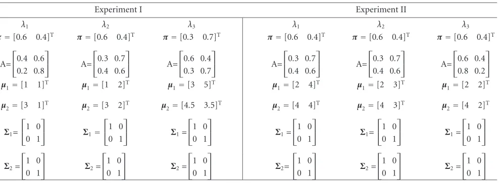
Table1: Model parameter settings of Gaussian HMMs.
Experiment I Experiment II
λ1 λ2 λ3 λ1 λ2 λ3
π=[0.6 0.4]T π=[0.6 0.4]T π=[0.3 0.7]T π=[0.6 0.4]T π=[0.6 0.4]T π=[0.6 0.4]T
A= 0.4 0.6
0.2 0.8
A=
0.3 0.7
0.4 0.6
A=
0.6 0.4
0.3 0.7
A=
0.3 0.7
0.4 0.6
A=
0.3 0.7
0.4 0.6
A=
0.6 0.4
0.8 0.2
µ1=[1 1]T µ1=[1 2]T µ1=[3 5]T µ1=[2 4]T µ1=[2 3]T µ1=[2 2]T
µ2=[3 1]T µ2=[3 2]T µ2=[4.5 3.5]T µ2=[4 4]T µ2=[4 3]T µ2=[4 2]T
Σ1= 1 0
0 1
Σ1=
1 0
0 1
Σ1=
1 0
0 1
Σ1=
1 0
0 1
Σ1=
1 0
0 1
Σ1=
1 0
0 1
Σ2= 1 0
0 1
Σ2=
1 0
0 1
Σ2=
1 0
0 1
Σ2=
1 0
0 1
Σ2=
1 0
0 1
Σ2=
1 0
0 1
We denoteS(2i)
as the unscaled 2i-step similarity tran-sition matrix,S(2i)
as the scaled 2i-step similarity transition
matrix, andS
(2i)
as the temporary matrix for the computa-tion ofS(2i)
. DenoteαTas the scaledαT. Below is the refined fast procedure embedded with the scaling procedure (again we assumeT=2n).
(1) Initialization.Computeα0andS. LetS (20)
=S. Let the
scaling coefficientc0be asc0 =(sum(S (20)
))−1, where
sum(S
(20)
) is the sum of all components of S
(20) . Let
S(20)
=c0S (20)
.
(2) Induction.LetS
(2i)
=S(2i−1) S(2i−1)
, andci=(sum(S
(2i) ))−1;
thenS(2i)
=ciS
(2i)
, for 1≤i≤n. HenceαT =α0S(T).
(3) Termination.From the induction step, it can be found that
S(T)=S(2n)=cnS
(2n)
= · · · =cnc2
1 n−1· · ·c2
n
0 S(2
n)
; (38)
then
αT=α0S(T)=α0cnc2 1 n−1· · ·c2
n
0S(2
n)
=cnc2
1 n−1· · ·c2
n
0 αT. (39) So the similarity measureKρ∗(λ,λ) is computed as
Kρ∗(λ,λ)=sum(αT)=
cnc2 1 n−1· · ·c2
n
0
−1
sum(αT
. (40)
BecauseKρ∗(λ,λ) andcnc2 1 n−1· · ·c2
n
0 will also go
be-yond the dynamic range of the machine, we need to take the logarithm
logKρ∗(λ,λ)
=logsumαT
−
n
i=0
2n−ilogci
. (41)
From the scaling procedure, for each 0≤i≤n, the values of the components of the scaled 2i-step similarity transition matrixS(2i)
are kept within the dynamic range of the com-puter by multiplying by a scaling coefficient ci. By exploit-ing the relationship between the scaled and unscaled simi-larity transition matrices (38), the exact logarithm value of
Kρ∗(λ,λ) is realized.
5. EXPERIMENTAL RESULTS
Our experiments include two parts. We first use simulated model parameters to test the effectiveness of the introduced similarity measure of Gaussian HMMs. Secondly we test the effectiveness on a set of real texture images for classification.
5.1. Experiments on simulated model parameters
In this subsection, we perform two experiments. In each ex-periment, three Gaussian HMMs are used to test their rela-tive similarity measure among each other. The model param-eters of the Gaussian HMMs are manually set. In the com-putation of similarity measures between Gaussians, we set
ρ=1/2, that is, Bhattacharyya’s measure of affinity between
Gaussians [9]. The similarity measure of all possible pairs of Gaussian HMMs among the three Gaussian HMMs are com-puted forT = 0, 1, 2, 22,. . ., 210.Table 1lists the model
pa-rameters chosen for these two experiments (also depicted in
Figure 1).
The setting of simulated model parameters is based on the consideration that it should be easy to make an in-tuitive judgment of the relative similarity between these models by just looking at the parameters of these mod-els. For example, by looking at Figure 1 and parameters in Table 1, one can intuitively tell that in experiment I,
K0.5(λ1,λ2)> K0.5(λ2,λ3)> K0.5(λ1,λ3); and in experiment
II,K0.5(λ1,λ2)> K0.5(λ2,λ3) > K0.5(λ1,λ3). Then in
5
4
3
2
1
0.3 1 0.7
2 0.6 0.4
0.3 1
0.7 2
0.6 0.4
0.3
1 0.7 2 0.6 0.4
1 2 3 4 5
(a)
5
4
3
2
1
0.3 1
0.7 2
0.6 0.4
0.3 1
0.7
2 0.6 0.4
0.3 1
0.7
2 0.6 0.4
1 2 3 4 5
(b)
Figure1: Gaussian HMMs used for experiments I and II.
that not only the similarities of pair 1-2 were always higher than those of pair 1-3 and pair 2-3, but also the magnitudes of the differences among these similarities increase exponen-tially overT(note that a logarithmic scale was used for the y-axis inFigure 2). This phenomenon suggests that with the in-crease ofT, the proposed similarity measure should become more accurate in classification.
5.2. Experiments on texture classification
In this subsection, the method of similarity measure of Gaussian HMMs is tested on texture classification. thirteen texture images of Brodatz texture images (see the USC-SIPI Image Database athttp://sipi.usc.edu/services/database/ Database.html) are used for classification; seeFigure 3. All 13 texture images are monochrome with size of 512×512. Each texture image is divided into 16 128×128 nonoverlapping sub-texture images for training and test.
−10−1
−100
−101
−102
−103 −104
0 2 8 32 128 512
T
logK0.5(1,2) logK0.5(1,3) logK0.5(2,3)
(a) −10−1
−100
−101
−102
−103
0 2 8 32 128 512
T
logK0.5(1,2) logK0.5(1,3) logK0.5(2,3)
(b)
Figure2: (a) and (b) Similarity measures of all possible pairs of Gaussian HMMs in Figures1aand1b, respectively.
Figure3: Thirteen categories of texture images. From top to bottom and from left to right, they are bark, brick, bubbles, grass, leather, pigskin, raffia, sand, straw, water, weave, wood, and wool.
5.2.1. Experiment one
In this experiment, for each class of texture, all 16 trained HMMs are selected for each class. Then totally there are 13×16=208 HMMs involved. The similarity measures of all possible pairs of HMMs among all selected 208 HMMs are computed withT =4 andρ =1/2.2Denotesi,j
m,nas the log of the similarity measure between themth HMM of class
iand thenth HMM of class j. The similarity measures are arranged by the following similarity measure matrix and de-picted inFigure 4a:
s1,11,1 s1,11,2 · · · s1,11,16 · · · s1,131,1 s1,131,2 · · · s1,131,16
s1,12,1 s1,12,2 · · · s1,12,16 · · · s1,132,1 s1,132,2 · · · s1,132,16
..
. ... ... ... ... ... ... ... ...
s13,116,1 s13,116,2 · · · s13,116,16 · · · s13,1316,1 s13,1316,2 · · · s13,1316,16
(42)
The brightness of each pixel inFigure 4arepresents the value of similarity measure of the corresponding pair of Gaussian HMMs, that is, the brighter the pixel, the greater the similar-ity measure.
It can be seen fromFigure 4athat within-class similarity measures are normally higher than between-class similarity measures, for example, the squares along the diagonal of the similarity measure matrix are generally brighter than the cor-responding off-diagonal squares. To illustrate this,Figure 4b
shows a sketch of squares along the diagonal of the similarity
2We excluded the influence of the initial probability distributionπby substituting allπi’s andπj’s with 1/N’s and 1/N’s. Due to the limited train-ing data (just one sub-texture image is used in the traintrain-ing of HMM), the initial probability distribution is unreliable and should be excluded from the computation of similarity measures.
measure matrix and the corresponding off-diagonal squares (the gray areas).
5.2.2. Experiment two
In this experiment, for each class of textures, 5 trained HMMs are randomly selected. The selected 5 HMMs of each texture class serve as class templates. All the corresponding unselected 11 trained HMMs of each class serve as the test-ing data. When an arbitrary testtest-ing HMM is sent to the clas-sification system, its similarity measures towards all the class templates of every texture class are computed. Then the sim-ilarity of the testing HMM towards a particular texture class is computed as the mean value of the similarity measures of the testing HMM towards all the 5 templates of that texture class. The identity of the testing HMM is assigned to the tex-ture class which has the highest similarity measure towards the testing HMM.
For the purpose of observing the convergence property of the similarity measure whenTgets big, we tested the recog-nition rates (the rates according to which the testing HMMs are correctly classified) onT =0, 20, 21, 22,. . ., 210; and the
ρ is set to be 1/2. When T = 0, the classification is actu-ally based on the similarity measure of the observation dis-tributions (Gaussian) of two HMMs and the state transition matrix is not involved in the computation. Obviously, when
Tgets big, the influence of the state transition matrix in the computation of similarity score gets big. The recognition rate whenT=0 is 0.8042. The recognition rates of other settings ofT’s values are depicted inFigure 5. An interesting obser-vation is that, in this experiment, the recognition rate jumps up from 0.8042 atT = 0 to 0.9510 at aroundT = 22, and
50
100
150
200
50 100 150 200
(a)
(b)
Figure4: (a) Similarity measure matrix of 13×16 Gaussian HMMs generated from 13×16 texture images. (b) Illustrative plot of squares along the diagonal of the similarity measure matrix and the corresponding off-diagonal squares.
HMM state distributions and the inaccuracy in model pa-rameter estimations. With texture images, the assumption of Gaussian model for our DCT domain feature vectors is mostly for computational simplicity; and the estimation of HMM model parameters for subimages from the same tex-ture class may not be consistent due to the variant appear-ances among these subimages (e.g., note the heterogeneous appearance in the straw image inFigure 3). The suboptimal property of the EM algorithm may also introduce some es-timation error. Furthermore, it is reasonable to assume that all three components of HMM model parameters (A,B,π) should share certain influence in determining the similarity measures. However, as stated in the previous subsection, π
is excluded from our experiment because of its inaccuracy due to limited training data. Therefore when T = 0, the similarity measure is solely determined byB. On the other
0.96 0.95 0.94 0.93 0.92 0.91 0.9
100 101 102 103 104
T
R
ec
o
gnition
rat
e
Figure5: Recognition rates whenTis set as 20, 21,. . ., 210.
hand, whenT→ ∞,Abecomes more and more dominant in the computation of similarity score. Therefore over the en-tire range ofT, there may be some point between 0 and∞
where the combination of contributions from AandBget maximized. Further studies will be conducted to address this phenomenon. When the bestTvalue is not known, a com-mon practice is to setTequal to the length of the observation sequences.
6. CONCLUSION
In this work, we introduced a similarity measure of Gaussian HMMs based on a modified “generalized probability product kernel” definition. We also provided a new interpretation for the derivation of this similarity measure. Two fast comput-ing procedures embedded with correspondcomput-ing scalcomput-ing proce-dures were presented. The similarity measure is evaluated on simulated model parameters as well as texture images. En-couraging results testified the effectiveness of the proposed method for similarity comparison between Gaussian HMMs. The method can be further generalized for the comparison of mixture Gaussian HMMs and more complicated stochas-tic models, and it may also find potential applications in other data analysis areas. The Matlab code for the proposed schemes will be available upon request.
ACKNOWLEDGMENT
The authors would like to thank the anonymous reviewers for their insightful comments and constructive suggestions.
REFERENCES
[1] F. Samaria,Face recognition using hidden Markov model, Ph.D. thesis, University of Cambridge, Cambridge, UK, 1995. [2] L. Chen, H. Man, and A. Nefian, “Face recognition based
[3] G. Fan and X.-G. Xia, “Wavelt-based texture analysis and syn-thesis using hidden Markov models,”IEEE Trans. Circuits Syst. I, vol. 50, no. 1, pp. 106–120, 2003.
[4] M. N. Do and M. Vetterli, “Rotation invariant texture charac-terization and retrieval using steerable wavelet-domain hid-den Markov models,”IEEE Trans. Multimedia, vol. 4, no. 4, pp. 517–527, 2002.
[5] B. H. Juang and L. Rabiner, “A probabilistic distance measure for hidden Markov models,”AT&T Technical Journal, vol. 64, no. 2, pp. 391–408, 1985.
[6] R. B. Lyngsø, C. N. S. Pedersen, and H. Nielsen, “Measures on hidden Markov models,” Technical Report RS-99-6, Basic Research in Computer Science, Aarhus, Denmark, 1999. [7] C. Bahlmann and H. Burkhardt, “Measuring HMM
similar-ity with the Bayes probabilsimilar-ity of error and its application to online handwriting recognition,” inProc. IEEE 6th Interna-tional Conference on Document Analysis and Recognition (IC-DAR ’01), pp. 406–411, Seattle, Wash, USA, September 2001. [8] T. Jebara and R. Kondor, “Bhattacharyya and expected likeli-hood kernels,” inProc. Conference on Learning Theory (COLT ’03), pp. 57–71, Washington, DC, USA, August 2003. [9] F. Aherne, N. Thacker, and P. Rockett, “The Bhattacharyya
metric as an absolute similarity measure for frequency coded data,”Kybernetika, vol. 32, no. 4, pp. 1–7, 1997.
[10] J. Schott,Matrix Analysis for Statistics, John Wiley & Sons, New York, NY, USA, 1996.
Ling Chen received the B.S. degree from the Northwestern Polytechnical University, China, in 1996, and the M.S. degree from the University of Electronic Science and Technology of China, China, in 1999, both in electrical engineering. Currently, he is a Ph.D. candidate in the Department of Elec-trical and Computer Engineering, Stevens Institute of Technology, Hoboken, New Jer-sey. His research interests include
biomet-rics, machine learning, statistical pattern recognition, and neural networks.
Hong Manreceived the B.S. degree from Soochow University, China, in 1988, the M.S. degree from Gonzaga University in 1994, and the Ph.D. degree from Georgia Institute of Technology in 1999, all in elec-trical engineering. He joined Stevens Insti-tute of Technology in 2000, and currently he is an Assistant Professor in the Department of Electrical and Computer Engineering. He is serving as the Director for Computer