Analysis of the IHC Adaptation for the
Anthropomorphic Speech Processing Systems
Alexei V. Ivanov
Computer Engineering Department, the Belarusian State University of Informatics and Radioelectronics, 220013 Minsk, Belarus
Email:alexei v [email protected]
Alexander A. Petrovsky
Real-Time Systems Department, the Bialystok Technical University, 15351 Bialystok, Poland Email:[email protected]
Received 1 November 2003; Revised 5 September 2004
We analyse the properties of the physiological model of the adaptive behaviour of the chemical synapse between inner hair cells (IHC) and auditory neurons. On the basis of the performed analysis, we propose equivalent structures of the model for implemen-tation in the digital domain. The main conclusion of the analysis is that the synapse reservoir model is equivalent in its properties to the signal-dependent automatic gain-control mechanism. We plot guidelines for creation of artificial anthropomorphic algo-rithms, which exploit properties of the original synapse model. This paper also presents a concise description of the experiments, which prove the presence of the positive effect from the introduction of the depicted anthropomorphic algorithm into feature extraction of the automated speech recognition engine.
Keywords and phrases:inner hair cell (IHC), Meddis IHC model, IHC adaptation, auditory models, modulation spectrum filter-ing.
1. INTRODUCTION
1.1. Anthropomorphism, psychoacoustics,
and auditory physiology
Many contemporary speech processing techniques tend to reflect properties of the human auditory apparatus. As a rule, most of the information about the way human beings process acoustic data comes into artificial applications from the field of psychoacoustics (for classical psychoacoustics work, refer to [1]).
Apart from the experiments with subjects that have re-liably diagnosed and anatomically localised auditory pathol-ogy, psychoacoustics treats the whole human auditory system as a “black box” and tries to infer its properties without par-ticular interest to its internal structure. Most of the psychoa-coustical experiments include analysis of the responses to “simple” sounds, like pure tones, wideband noise, coloured noises, clicks, and so forth. But a lot of evidence (simulta-neous and nonsimulta(simulta-neous masking, pitch perception, etc.) points to the fact that the auditory system is essentially a non-linear system.
From the system identification theory, it is known that the response of the linear system to an arbitrary excitation can be derived from the study of responses of such sys-tem to simple sounds, for example, tones, noises, and clicks.
There is no need to study the internal structure of the lin-ear black box as far as responses to the simple input signals are known. Strictly speaking, for the case of nonlinear sys-tems, this black box approach is not applicable. There are mainly two possibilities to model a nonlinear system: either to construct a semiparametric statistical learning machine, a “neural-network-like” structure, and let it adapt through a kind of learning algorithm, or follow the parametric ap-proach and somehow infer the internal structure of the non-linear system to be modelled, parse it into smaller and, hope-fully, simpler building blocks, then tune parameters of those blocks, so that model response matches that of the original system.
The first alternative suffers from the problems in creating the representative training set, as well as from the absence of a priori information regarding the required model com-plexity. The mentioned difficulties virtually prohibit applica-tion of this approach to the auditory modelling. The second of the mentioned approaches corresponds to the physiologi-cally grounded studies of the auditory apparatus.
speech recognition applications. While the first two men-tioned branches are concentrated on the closest possible lit-eral reproduction of the auditory apparatus properties in the artificial device, the latter imply a computationally efficient way to implement the “biological” audio processing algo-rithm with a certain predefined precision.
In spite of being precise and objective, the physiological hearing models neither provide a clear signal processing in-terpretation of those phenomena, nor give a ready answer regarding the relevance of the modelled phenomena to the hearing process in general. Thus, straightforward applica-tion of the physiological models to the fields of audio coding and speech recognition may not easily gain advantage over the conventional algorithms [2]. Before the employment of a certain physiological model into the mentioned applications, one should answer the questions of why it is important (i.e., what result is expected from it) and what is the most efficient way of its implementation. This reasoning leads to a conclu-sion that the further analysis of the available physiological models with the aim of finding their algorithmical interpre-tation is needed. This paper is further devoted to such kind of analysis.
Particularly, we are aiming at analysing the adaptation of the chemical “inner-hair-cell auditory nerve” (IHC-AN) synapse, and trying to infer its importance to the artificial an-thropomorphic audio signal (and particularly speech) pro-cessing systems in adverse environments. Indeed, strong on-set responses of the auditory nerve (AN) fibers to the pre-sented stimulus are followed by the “adaptation”, that is, gradual decrease of the response amplitude over time while the stimulus amplitude remains constant. This “adaptive strategy” at first glance seems to be advantageous since it al-lows an emphasis of nonstationarities within the incoming signal.
2. RESERVOIR MODEL OF IHC-AN CHEMICAL SYNAPSE
Physiological research into the way the inner ear converts an acoustical stimulation into a response of the auditory nerve fibers (for a brief summary and review, refer to [3]) among many other findings led to the conclusions that
(i) inner hair cells are mechanical vibrations sensory cells; (ii) each IHC makes chemical synapses with approxi-mately 10–30 peripheral axons of primary bipolar neu-rons which cell bodies contained in the spiral gan-glion and modiolar axons forming the auditory (VI-IIth) nerve;
(iii) one can distinguish three groups of afferent neu-rons based on the level of their spontaneous activity: low-spontaneous rate, medium-spontaneous rate, and high-spontaneous rate fibers. The level of spontaneous activity of the fiber is closely related to the form and the size of the synapse it formed with IHC;
(iv) chemical nature determines the following properties of IHC-AN synapses: adaptive responses, synaptic delays, quantised response amplitudes.
Reprocessing storew(t) Free transmitter
poolq(t) Transmitter factory
Synaptic cleft c(t)
Postsynaptic afferent auditory
nerve fiber Loss
Hair cell lc(t)
rc(t) k(t)q(t) xw(t)
y[M−q(t)]
Figure1: Schematic representation of the Meddis reservoir model.
Properties of the chemical IHC-AN synapse are success-fully captured by the so-called “reservoir models,” in which neurotransmitter is produced and stored in the IHC to be re-leased in accordance with IHC transmitter release probabil-ity that changes with mechanical vibrations in the inner ear. First reservoir models for IHC-AN synapses were proposed as early as [4,5].
Meddis has put forward [6] and further developed [7,8, 9,10,11] a model of IHC, which includes a version of reser-voir model of chemical synapse. The latest model [10,11] allows for a nice fit between experimental and model data for all thee groups of IHC-AN synapses (low-, medium-, and high-spontaneous rate fibers) with only calcium conduc-tance parameters being changed.
It must be noted here that in reality neurotransmitter re-lease into synaptic cleft is a probabilistic and quantal process. However, to a certain degree, the dynamical properties of the synapse may be reflected by the model that assumes that neu-rotransmitter flow is deterministic and continuous. From the practical point of view, this assumption corresponds to the averaging of the synapse response over many identical stimu-lations. Latest Meddis models [9,10,11] depart from this as-sumption offering better correspondence to the data record-ings of individual experiments. For the purpose of the anal-ysis of the core properties of IHC-AN synapse and construc-tion of the anthropomorphic artificial algorithms, we further narrow our consideration to the deterministic and continu-ous case.
We assume that the pool capacity equalsM. The quantity of the transmitter stored in the pool at a certain time instant will be denoted byq(t). The rate, at which the factory pro-duces new transmitter, is proportional to the free volume of the pool y[M−q(t)], here operation [· · ·] constitutes the choice of the biggest value between zero and the value inside square brackets. Alternatively we may put that coefficienty becomes zero at the moment the pool is filled to the limit. We denote the instantaneous amount of the transmitter in the reprocessing byw(t). The recirculation rate is proportional to the amount of the transmitter in the reprocessingxw(t). The rate, at which transmitter is sent to the cleft, is equal to the product of membrane permeabilityk(t) and the quantity of the transmitter in the poolq(t). The quantity of the neu-rotransmitter in the cleft at certain instant will be denoted by c(t). Rates of neurotransmitter loss and return for reprocess-ing are proportional to the amount of the transmitter in the cleftslc(t) andrc(t), respectively.
As it follows from the above-presented description, Med-dis version of the reservoir model is described by the follow-ing set of differential equations:
dq(t)
dt =xw(t) +y
M−q(t)−k(t)q(t),
dc
dt =k(t)q(t)−(l+r)c(t), dw
dt =rc(t)−xw(t).
(1)
Initial conditions of the model are taken in accordance with the assumption that at a certain instantt0the system is in an equilibrium state:
xwt0
+yM−qt0
=kt0
qt0
,
kt0
qt0
=(l+r)ct0
,
rct0
=xwt0
.
(2)
3. ADAPTATION PROPERTY OF THE RESERVOIR MODEL OF IHC-AN CHEMICAL SYNAPSE
Figure 2presents a typical response of the Meddis model to the excitation. Signalk(t) is an input to the reservoir model and is computed by earlier stages of cochlear model (the cochlear filter bank [12] in combination with the first part of IHC model [10]) when the test tone of 6 kHz is presented. IHC medium-spontaneous rate fiber model gets its input from the cochlear filter bank section with the closest to 6 kHz centre frequency. It is running at the sampling frequency of 16 kHz.
Typical values of the model coefficients were taken from the works of Meddis [6,7,8,9] and are as follows:
M=10, x=66.3, y=10,
l=2580, r=6580. (3)
0 0 0 0
500 500 500 500
1000 1000 1000 1000
1500 1500 1500 1500
2000 2000 2000 2000
2500 2500 2500 2500
3000 3000 3000 3000
3500 3500 3500 3500
4000 4000 4000 4000
2 3 4 0 0.05 0.1 1 2 3 4 0 100 200
300 A B C D
w
(
t
)
c
(
t
)
q
(
t
)
k
(
t
)
Time
Figure2: Reservoir model response to the excitation with the 6 kHz tone, CF∼6 kHz,Fs=48 kHz, medium-spontaneous rate fiber. A: steady state, B: onset, C: adaptation, D: offset.
In order to perform this digital simulation (depicted in Figure 2) of the synapse model, the forward difference ap-proximation of the set of differential equations (1) was used, as it is advised in [8].
As it can be seen from the above figure, there are four dis-tinct regions in the model response signal c(t): steady-state response to a long-term absence of stimulation (denoted as region A); onset response (region B)—brief rise of the re-sponse level to higher values; subsequent adaptation of the response level to a much lower activity (region C); offset region (region D), when synapse recovers from the stimu-lation and response level slowly converges to a steady-state level.
For a detailed review of adaptation properties of IHC, please refer to [11].
4. ANALYSIS OF THE RESERVOIR MODEL OF IHC-AN CHEMICAL SYNAPSE
Looking at the equation set (1), one can easily notice that functionsc(t) and f(t) = k(t)q(t) are linked with the lin-ear constant-coefficient differential equation of the first or-der with zero-free member:
dc(t)
dt + (l+r)c(t)=f(t). (4)
0 1000 2000 3000 4000 5000 6000 7000 8000 −88
−86 −84 −82 −80 −78
M
ag
nitude
(dB)
Frequency (Hz)
0 1000 2000 3000 4000 5000 6000 7000 8000 −200
−150 −100 −50 0
Phase
(deg
rees)
Frequency (Hz)
Figure3: Frequency characteristic of filter A (Fs=16 kHz).
a digital filter:
c(n)= 1
Fsf
(n−1)−
l+r−Fs
Fs c
(n−1), (5)
HA=
(1/Fs)z−1
1−1−(l+r)/Fs
z−1. (6)
HereFsdenotes the sampling frequency. We will further
refer to this filter as “filter A.” With the typical values of parametersl andr, this filter is a lowpass filter, which has rather smooth slope response characteristic that is presented inFigure 3.
Further analysis of the equation set (1) leads to a con-clusion that functionss(t)=M−q(t) and f(t)=k(t)q(t) are also linked with the linear constant-coefficient diff eren-tial equation of the first order with zero-free member:
d3s(t)
dt3 + (x+y+l+r) d2s(t)
dt2 +
(x+y)(l+r) +xyds(t) dt
+xy(l+r)s(t)=d2f(t)
dt2 + (x+l+r) df(t)
dt +xl f(t). (7)
We note that this equation is valid for all such values s(t)=M−q(t)≥0. Ifs(t)=M−q(t)≤ 0, then it must be substituted with the following equation, which is obtained from (7) by lettingy=0:
d3s(t)
dt3 + (x+l+r) d2s(t)
dt2 +x(l+r) ds(t)
dt
=d2f(t)
dt2 + (x+l+r) df(t)
dt +xl f(t).
(8)
The performed digital simulations show that for realistic input signals and reasonably high sampling frequency, it is enough to use (7) only.
0 1000 2000 3000 4000 5000 6000 7000 8000 −100
−90 −80 −70 −60 −50 −40 −30
M
ag
nitude
(dB)
Frequency (Hz)
0 1000 2000 3000 4000 5000 6000 7000 8000 0
50 100 150 200
Phase
(deg
rees)
Frequency (Hz)
Figure4: Frequency characteristic of filter B (Fs=16 kHz).
Again it is possible to approximate the system described by (7) with a digital filter:
s(n)=b1 a0f
(n−1) +b2 a0f
(n−2) +b3 a0f
(n−3)
−a1 a0s
(n−1)−a2 a0s
(n−2)−a3 a0s
(n−3),
a0=Fs3,
a1= −3Fs3+Fs2(x+y+l+r),
a2=3Fs3−2Fs2(x+y+l+r) +Fs
(x+y)(l+r) +xy,
a3= −Fs3+Fs2(x+y+l+r)
−Fs
(x+y)(l+r) +xy+xy(l+r),
b1=Fs2,
b2= −2Fs2+Fs(x+l+r),
b3=Fs2−Fs(x+l+r) +xl.
(9)
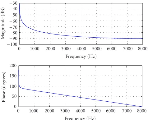
We denote this filter as “filter B.” This is a lowpass fil-ter with rather sharp frequency response characfil-teristic (see Figure 4) for typical values of parametersx,y,l, andr.
Filter B has two real zeros and three real poles:
nB1,2=1− 1 2Fs
(x+l+r)±(x+l+r)2−4xl, (10)
pB1=1−l+r Fs
, pB2=1− x
Fs
, pB3=1− y
Fs.
(11)
0 1000 2000 3000 4000 5000 6000 7000 8000 −50
−40 −30 −20 −10 0 10
M
ag
nitude
(dB)
Frequency (Hz)
0 1000 2000 3000 4000 5000 6000 7000 8000 180
200 220 240 260 280
Phase
(deg
rees)
Frequency (Hz)
Figure5: Frequency characteristic of filter C (Fs=16 kHz).
of the linear constant-coefficient differential equation of the first order with zero-free member. Indeed, it is the case
d2c(t)
dt2 + (x+l+r) ds(t)
dt +xlc(t)
= −d2s(t)
dt2 −(x+y) ds(t)
dt +xys(t).
(12)
As in the case of (7), this equation is valid fors(t)=M−
q(t)≥0, if it is less than zero, thenyin (12) should be put to zero.
The digital filter, which is equivalent to the system (12), is defined as follows:
s(n)=d0 c0f
(n) +d1 c0 f
(n−1) +d2 c0 f
(n−2)
−c1 c0s
(n−1)−c2 c0s
(n−2),
c0=Fs2,
c1= −2Fs2+Fs(x+l+r),
c2=Fs2−Fs(x+l+r) +xl,
d0= −Fs2,
d1=2Fs2−Fs(x+y),
d2= −Fs2+Fs(x+y)−xy.
(13)
We will further denote this filter as “filter C.” It is a high-pass filter with rather sharp frequency response characteristic (seeFigure 5) for typical values of its parameters.
We also note that a cascade connection of filters B and C should be equivalent to filter A. This is true and can be immediately proved by looking at (9), (13), and (5).
Filter A Filter B
Filter B Filter C k(t)
k(t)
+ +
− −
s(t) s(t)
k(t)q(t) k(t)q(t)
M M
c(t) c(t)
Figure6: Reservoir model equivalent structures.
5. EQUIVALENT DIGITAL STRUCTURES FOR THE RESERVOIR MODEL
Analysis of the Meddis reservoir model allows us to plot its equivalent structures for realisation in the digital form (see Figure 6). The realisation with the help of filter A is more preferable since it is more computationally efficient.
Apart from the linear digital filters, the developed equiv-alent representations include an operation of multiplica-tion of the signals in the time domain. It should be noted that, in general, multiplication of time-varying signals does not comply with the superposition principle, thus the reser-voir model equivalent structure performs a nonlinear signal transformation. The signalq(t)=M−s(t), which is multi-plied byk(t) is confined in the interval [0,M] in accordance with the reservoir model definition. It consists mainly of low-frequency components of signalk(t)q(t) in accordance with the properties of filter B.
Operation of the multiplication in the equivalent struc-ture may be viewed as an automatic gain-control (AGC) op-eration. The gain q(t) is a parameter, which slowly varies through time betweenMin the case of weak input signal and zero in the case of strong one.
Our equivalent structure of the Meddis reservoir model has similarities with that plotted in the works of Perdigao [13, 14].
6. LINEAR APPROXIMATION OF THE SIGNAL
MULTIPLICATION OPERATION IN THE EQUIVALENT STRUCTURE OF THE RESERVOIR MODEL
It is possible to build a linear digital filter, which approxi-mates the effect of the AGC mechanism for the case of small deviations of the system from the equilibrium state. Partic-ular form of such filter is dependent on initial conditions, namely, the steady-state input signal valuek0.
Indeed, we assume that the system depicted inFigure 6, at a certain time instant, resides in the equilibrium. For such case, we may write
f0=k0q0, q0=M−s0, y(l+r)s0=l f0.
(14)
Any deviations from the steady state are sufficiently small:
k(n)=k0+δk(n), f(n)= f0+δ f(n), q(n)=q0+δq(n), s(n)=s0+δs(n).
(15)
Thus, for such system at an arbitrary time instant, we may write the following set of equations (seeFigure 6):
f0+δ f(n)=
k0+δk(n)
q0+δq(n)
,
q0+δq(n)=M−
s0+δs(n)
,
a0+a1+a2+a3
s0+a0δs(n) +a1δs(n−1) +a2δs(n−2)
+a3δs(n−3)=
b1+b2+b3
f0+b1δ f(n−1)
+b2δ f(n−2) +b3δ f(n−3).
(16)
Coefficients in the third equation of the set are those of filter B. Comparing sets (15) and (16), we may conclude that the following set of equations holds for deviations:
δ f(n)=k0δq(n) +q0δk(n), δq(n)= −δs(n),
a0δs(n) +a1δs(n−1) +a2δs(n−2) +a3δs(n−3) =b1δ f(n−1) +b2δ f(n−2) +b3δ f(n−3).
(17)
A solution of the equation set (17) with respect to vari-ablesδk(n) andδ f(n) is represented as
q0= M y(l +r) y(l+r) +lk0
,
q0
a0δk(n) +a1δk(n−1) +a2δk(n−2) +a3δk(n−3)
=a0δ f(n) +
b1k0+a1
δ f(n−1)
+b2k0+a2
δ f(n−2) +b3k0+a3
δ f(n−3). (18)
This equation represents a desired linear digital filter, which linearly approximates AGC of the equivalent struc-ture. This filter is capable of transforming the signalδk(t)=
k(t)−k0 into δ f(t) = δ(k(t)q(t)) = f(t)− f0 under the
0 200 400 600 800 1000 1200 1400 1600 1800 2000 15.5
16 16.5 17 17.5 18
M
ag
nitude
(dB)
Frequency (Hz)
0 200 400 600 800 1000 1200 1400 1600 1800 2000 0
1 2 3 4 5
Phase
(deg
rees)
Frequency (Hz)
Figure7: Frequency characteristic of filter D (Fs =16 kHz,k0 =
10).
condition that these deviations are sufficiently small. The transfer function of this filter is expressed as
HD
z,k0
= M y(l+r) y(l+r) +lk0
· a0+a1z−1+a2z−2+a3z−3 a0+
b1k0+a1
z−1+b
2k0+a2
z−2+b
3k0+a3
z−3.
(19)
Note the explicit dependency of the form of this transfer function on the value ofk0. We will further denote this filter as “filter D.”
The steady-state output f0(k0) of the system is derived from the equilibrium set of (14) and is expressed as
f0
k0
=q0k0= M y (l+r) y(l+r) +lk0k0.
(20)
Filter D is a highpass filter with quite sharp frequency response characteristic (see Figure 7) for a typical value of k0=10.
In order to illustrate the dependence of the properties of filter D upon the value ofk0,Figure 8depicts frequency char-acteristic of that filter withk0=1000. As it can be seen from the comparison of Figures7and8, apart from the change of the gain, the cut-offfrequency of the filter is getting bigger with the increase ofk0.
0 200 400 600 800 1000 1200 1400 1600 1800 2000 −40
−35 −30 −25 −20 −15 −10 −5
M
ag
n
itude
(dB)
Frequency (Hz)
0 200 400 600 800 1000 1200 1400 1600 1800 2000 0
10 20 30 40 50 60 70
Phase
(deg
rees)
Frequency (Hz)
Figure8: Frequency characteristic of filter D (Fs =16 kHz,k0 =
1000).
An alternative way is to estimate positions of the filter poles. Indeed, for realistic values ofk0 ∼101–102with quite good precision, filter D poles lay in the vicinity of its zeros. Zeros of filter D coincide with poles of filter B (11), and ap-proximately we may put
pD1≈nD1=1−l+r Fs
, pD2≈nD2=1− x Fs
,
pD3≈nD3=1− y Fs.
(21)
It must be noted also that ifk0→0, thenpDN→nDN.
Pole pD1 first leaves the unit circle while sampling fre-quency is being decreased, indeed the realistic values ofl+r are significantly larger than the values of x and y. Conse-quently, approximation of the position of the first pole gives us a condition of filter D stability, whilek0→0:
Fs>l+r
2 . (22)
PolepD1moves to the right on the real axis if the value of k0is being increased. This allows for filter D to become stable with increasedk0even if it was unstable with the smaller val-ues ofk0. This leads us to a conclusion that (22) represents sufficient condition for filter D to be stable with arbitrary re-alistic values ofk0.
In the work [8], it is required that the sampling frequency must be sufficiently large for a successful digital implemen-tation of the reservoir model. Our finding of stability con-dition (22) puts a quantitative restriction on the sampling frequency for the linearised approximation.
Under the same assumption of small deviations from the equilibrium state, it is possible to construct an equivalent lin-ear filter, which would serve as linlin-ear approximation of rela-tion of the signalsδk(t) andδc(t)=c(t)−c0, that is, the in-put and the outin-put signals of the reservoir model measured relatively to their corresponding equilibrium values.
Such filter (further denoted as filter E) corresponds to the cascade of the filters D and A. Its frequency response charac-teristic is presented inFigure 9. Filter E transfer function is defined as
HE
z,k0
= 1
FS ·
M y(l+r)
y(l+r) +lk0 ·
1−nD2z−1
1−nD3z−1
z−1 1 +b1k0+a1
/a0
z−1+b
2k0+a2
/a0
z−2+b
3k0+a3
/a0
z−3. (23)
It should be noted that the pole of filter A and the first zero of filter D are equal, thus they are removed from (23).
Response magnitude in the equilibrium state is derived from (2) and (20) and it looks like
c0
k0
= 1
(l+r)f0
k0
= M y
y(l+r) +lk0k0.
(24)
The notion that poles of filter E coincide with those of filter D leads to a conclusion that condition of the stability of the filter is identical to that of filter D.
7. PRACTICAL OUTCOME OF THE PRESENTED RESERVOIR MODEL ANALYSIS
As it can be seen fromFigure 6, the reservoir model is equiv-alent to a kind of signal-dependent gain-control mechanism. The presented equivalent structure may be perceived as the interpretation of the IHC adaptation mechanism from the
algorithmical signal processing point of view. In the equiva-lent structure, filters A, B, and C are all linear time-invariant structures, the only nonlinear element here is the multiplica-tion of the signals. Implementamultiplica-tion of the equivalent struc-ture via a combination of filters A and B seems more prefer-able among the alternatives, presented in Figure 6, since it requires less computational effort.
0 1000 2000 3000 4000 5000 6000 7000 8000 −76
−74 −72 −70 −68 −66
M
ag
nitude
(dB)
Frequency (Hz)
0 1000 2000 3000 4000 5000 6000 7000 8000 −200
−150 −100 −50 0 50
Phase
(deg
rees)
Frequency (Hz)
Figure9: Frequency characteristic of filter E (Fs = 16 kHz,k0 =
50).
realistic values of the model parameters. Indeed, such limi-tation of the lowest possible sampling frequency makes effi -cient combination of the model with multirate cochlear filter banks impossible.
Fortunately, there exist other methods of approximation of the differential problem in the digital domain, for exam-ple, bilinear transformation. In accordance with its proper-ties, any stable analog linear time-invariant filter, described by the corresponding differential equation, is converted into a stable digital filter. With the help of bilinear transforma-tion, it is possible to construct universally stable digital fil-ters A and B regardless of the sampling frequency. This pro-cedure as well as its combination with computationally effi -cient implementation of the multirate cochlear filter bank is described in detail in [19].
However, in the case of bilinear transformation, unlike the situation with difference approximation, the coefficient b0of the filter B is not equal to zero:
HB(z)= b0+b1z
−1+b
2z−2+b3z−3
a0+a1z−1+a2z−2+a3z−3 ,
a0=8Fs3+ 4Fs2(x+y+l+r) + 2Fs
(x+y)(l+r) +xy+xy(l+r),
a1= −24Fs3−4Fs2(x+y+l+r) + 2Fs
(x+y)(l+r) +xy+ 3xy(l+r),
a2=24Fs3−4Fs2(x+y+l+r) −2Fs
(x+y)(l+r) +xy+ 3xy(l+r),
a3= −8Fs3+ 4Fs2(x+y+l+r) −2Fs
(x+y)(l+r) +xy+xy(l+r),
b0=4Fs2+ 2Fs(x+l+r) +xl,
b1= −4Fs2+ 2Fs(x+l+r) + 3xl,
b2= −4Fs2−2Fs(x+l+r) + 3xl,
b3=4Fs2−2Fs(x+l+r) +xl.
(25)
M
f(n)
z−1 z−1 z−1 b0/a0
b1/a0 a1/a0
a2/a0 b2/a0
b3/a0 a3/a0 k(n)
1 +b0 a0k(n)
Figure10: Transposed direct form II realization.
This fact leads to the additional operations at the imple-mentation of the signal flow of Figure 6. Indeed, writing a set of equations describing the signal flow over the feedback loop ofFigure 6results in the following relations:
f(n)=k(n)q(n)=k(n)M−s(n), 3
i=0
bif(n−i)= 3
i=0
ais(n−i).
(26)
It is evident that simple substitution of the second equa-tion into the first does not lead to the expression of the out-put signal f(n) through the current value of the input signal k(n) and previous values of the signals f ands. The current value of the output is present on the both sides of the equa-tion. Separation of the variables leads to the following ex-pression for the output signal:
f(n)= k(n)
1+b0/a0
k(n)· M−3
i=1 bi
a0f (n−i)+
3
i=1 ai
a0s (n−i)
.
(27)
It appears that the most computationally effective way to implement filter B with its signal feedback is a transposed di-rect form II structure (Figure 10). This realisation minimises the number of delay units.
For the sake of completeness of the picture, the follow-ing formula presents a version of the digital filter A, which is obtained with the help of bilinear transformation:
HA(z)=
1 l+r+ 2Fs·
1 +z−1 1 +l+r−2Fs
/l+r+ 2Fs
z−1.
(28)
Linear approximation (23) of the reservoir model might be viewed as a computationally effective way to implement the model when input signal does not significantly deviate from a certain fixed stationary value. It might also serve as the linear time-variant filter, which simulates the reservoir model, when the slowly varying stationary value of the signal k0is known in advance or is estimated through a long-term moving average procedure.
This linear approximation is also important because of its link to the RASTA filtering technique [20,21], a well-established channel normalisation and speech augmentation means in ASR. Although the nature of this link needs further investigation, both techniques represent low-passband filters, running in separate frequency channels, which are converted with the help of nonlinearity. In the case of RASTA, each fre-quency channel is decimated to represent one frefre-quency bin of the short time Fourier transform spectrogram and con-verted into modulation-frequency domain by Jah-log trans-formation [16]. In the case of reservoir model there is no explicit decimation and the passband signal is transformed by “BM vibration—membrane permeability” transforma-tion [6], which somewhat resembles Jah-log transform.
8. EXPERIMENTS
Several experiments were run in order to validate the orig-inal assumption that the anthropomorphic auditory mod-elling in general and IHC adaptation model in particular may indeed augment performance of the ASR systems. A compar-ison involved three experimental setups, which are described in more detailed fashion in [22].
(i) BASELINE: an ASR feature extraction (FE) algorithm, which is based on linear time-invariant perceptually aligned filters.
(ii) A-MORPHIC: anthropomorphic feature extraction al-gorithm [22], which combined linear time-variant cochlear filters to model auditory suppression and the above-described IHC reservoir model implemen-tation. However, results mainly reflect effect of the IHC reservoir model since speech recordings in the ex-periment had approximately the same loudness level (∼40 dB SPL).
(iii) RASTA: the conventional RASTA algorithm-based fea-ture extraction [16].
In order to be effective, ASR FE algorithms should con-vey as much information about the speech source as possible. The measure of the amount of conveyed information, that is, the mutual information between a speech sourceS, which at any instant of time resides in one of the possible states Ci,
i=1, 2,. . .,N, and a measured feature vector componentX is defined as follows:
I(S,X)=H(S)−H(S|X)
= −
∀Ci∈{c}
PCi
log2PCi
+
∀Ci∈{c}
G(X)P
Ci,X
log2PCi|X
dX.
(29)
c0 c2 c4 c6 c8
dc1 dc3 dc5 dc7 ddc0 ddc2 ddc4 ddc6 ddc8 0
0.1 0.2 0.3 0.4 0.5 0.6 0.7 0.8 0.9 0.9 1
M
u
tual
infor
mation
(bits)
Features BASELINE
A-MORPHIC RASTA
Figure11: Mutual information of feature components (∆X=0.01).
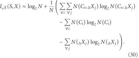
Estimation of the mutual information has been per-formed with the help of the following procedure [22]:
I∆X(S,X)≈log2N+ 1 N
∀i
∀j
NCi,∆Xj
log2NCi,∆Xj
−
∀i
NCi
log2NCi
−
∀j
N∆Xj
log2N∆Xj
.
(30)
Here N denotes a total number of feature frames
in the measurement; N(∆Xj)—a number of frames when
the feature value falls into the interval [min(X) + (j −
1)∆X, min(X) + j∆X]; N(Ci)—a number of frames which
were generated in the state Ci; N(Ci,∆Xj)—a number of
frames, belonging to the certain feature interval, which were generated by the source in the stateCi.
Phonetically labelled TIMIT speech corpus was used in this experiment. Probability distributions were approx-imated with histograms that had a step size ∆X = 0.01. Results, which are presented in Figure 11, show that A-MORPHIC features are generally the most informative.
Another experiment was performed to estimate a degree of invariance of the feature vectors to different kinds of ad-verse interference. To provide estimates of the feature invari-ance degree a simple Euclidian distinvari-ance between feature vec-tors was used. Exact experiment description may be found in [22]. Results of the experiment, which are presented in Table 1, reflect a mean distance of the feature vectors in ad-verse conditions to those perceived in a “clean” environment. As it can be seen from the table, A-MORPHIC features are less invariant to the adverse interference than RASTA. Any-way, a distance between “clean” and severely noisy (SNR 0 dB) features in the case of A-MORPHIC FE matches that between “clean” and mildly-noisy (SNR 30 dB) features in the BASELINE case.
Table1: Expected mean distance between the feature vectors in ad-verse conditions and clean environment.
Feature extraction algorithm
Interference
Noise Noise Noise Convol.
30 dB 10 dB 0 dB channel
BASELINE 0.41597 0.78894 1.05047 0.49298 RASTA FE 0.09842 0.17563 0.22338 0.05300 A-MORPHIC 0.26853 0.44951 0.42615 0.16665
performances (refer to [23] for a description of the recog-niser). It’s main result is that in adverse environments the recogniser with A-MORPHIC FE performs at least as good as the one with RASTA FE. These facts support the conjecture of the present paper that application of the anthropomor-phic algorithms in technical devices, namely, ASR engines, is fruitful.
9. CONCLUSIONS
Analysis of the physiological model of the chemical IHC-AN synapse creates an opportunity to implement it in the form of the anthropomorphic algorithm, which is computation-ally efficient and thus may be used in technical devices. The equivalent digital and linearised equivalent representations create alternatives for a traditional direct difference approx-imation of the original set of differential equations. These representations allow for a multiple “accuracy versus compu-tational load” tradeoffs at the implementation stage. Within the described framework, it is possible to create implementa-tions, which remain stable regardless to the signal sampling frequency.
It was found that effect of the IHC adaptation model is equivalent to the action of signal-dependent automatic gain control mechanism. It is also conjectured that effect of the linearised equivalent representation resembles that of RASTA, an algorithm engineered with the aim of alleviating the influence of additive and convolutive noises. This inter-pretation of the IHC-AN synapse model gives us reasons to believe that it is important as a mean of increasing ASR ro-bustness to the real-world environments (e.g., “too slow” and “too fast” varying additive and convolutive noises) and also as a mean of enhancement of the useful signal in the speech coding applications. Presented and referenced experiments confirm viability of the application of the discussed anthro-pomorphic algorithm to the ASR field. However, the exact form of the relation between the IHC-AN synapse model and RASTA should be investigated further.
ACKNOWLEDGMENTS
The authors would like to thank G. Kubin and the anony-mous reviewers for the valuable insights they provided as this article was developed. This work is supported in part by the Bialystok Technical University under the Grant no. W/WI/02/03.
REFERENCES
[1] E. Zwicker and H. Fastl, Psychoacoustics, Facts and Models, Springer, Berlin, Germany, 1990.
[2] H. Hermansky, “Should recognizers have ears?”Speech Com-munication, vol. 25, no. 1, pp. 3–27, 1998.
[3] D. C. Geisler,From Sound to Synapse: Physiology of the Mam-malian Ear, Oxford University Press, New York, NY, USA, 1998.
[4] M. R. Schroeder and J. L. Hall, “Model for mechanical to neural transduction in the auditory receptor,”Journal of the Acoustical Society of America, vol. 55, no. 5, pp. 1055–1060, 1974.
[5] Y. Oono and Y. Sujaku, “A model for automatic gain control observed in the firings of primary auditory neurons,”Abstracts of IECE Transactions, vol. 58, no. 6, pp. 61–62, 1975.
[6] R. Meddis, “Simulation of mechanical to neural transduction in the auditory receptor,”Journal of the Acoustical Society of America, vol. 79, no. 3, pp. 702–711, 1986.
[7] R. Meddis, “Simulation of auditory-neural transduction: Fur-ther studies,” Journal of the Acoustical Society of America, vol. 83, no. 3, pp. 1056–1063, 1988.
[8] R. Meddis, M. J. Hewitt, and T. M. Shackleton, “Implemen-tation details of a compu“Implemen-tation model of the inner hair-cell auditory-nerve synapse,”Journal of the Acoustical Society of America, vol. 87, no. 4, pp. 1813–1816, 1990.
[9] E. A. Lopez-Poveda, L. P. O’Mard, and R. Meddis, “A revised computational inner hair cell model,” inProc. 11th Interna-tional Symposium on Hearing, pp. 112–121, Grantham, UK, August 1997.
[10] C. J. Sumner, E. A. Lopez-Poveda, L. P. O’Mard, and R. Med-dis, “A revised model of the inner-hair cell and auditory-nerve complex,”Journal of the Acoustical Society of America, vol. 111, no. 5, pp. 2178–2188, 2002.
[11] C. J. Sumner, E. A. Lopez-Poveda, L. P. O’Mard, and R. Med-dis, “Adaptation in a revised inner-hair cell model,”Journal of the Acoustical Society of America, vol. 113, no. 2, pp. 893–901, 2003.
[12] A. Ivanov and A. Petrovsky, “Auditory models for robust fea-ture extraction: suppression,” inProc. IEEE Signal Processing Workshop, pp. 23–28, Poznan, Poland, October 2003. [13] F. S. Perdigao and L. V. Sa, “Properties of auditory model
rep-resentations,” inProc. European Conference on Speech Com-munication and Technology (EUROSPEECH ’97), vol. 5, pp. 2499–2502, Rhodes, Greece, September 1997.
[14] F. S. Perdigao and L. V. Sa, “Auditory models as front-ends for speech recognition,” inProc. NATO Advanced Study Institute on Computational Hearing, Il Ciocco, Italy, July 1988. [15] D. N. Morgan, “On discrete-time AGC amplifiers,” IEEE
Trans. Circuits Syst., vol. 22, no. 2, pp. 135–146, 1975. [16] A. H¨arm¨a and K. Palom¨aki, “HUTear—a free Matlab toolbox
for modeling of human auditory system,” inProc. 1999 MAT-LAB DSP Conference, pp. 96–99, Espoo, Finland, November 1999.
[17] M. Slaney, “Auditory toolbox, version 2,” Tec. Rep. 1998-10, Interval Research Corporation, Palo Alto, Calif, USA, 1998. [18] R. D. Patterson and M. H. Allerhand, “Time-domain
mod-elling of peripheral auditory processing: a modular architec-ture and a software platform,”Journal of the Acoustical Society of America, vol. 98, no. 4, pp. 1890–1894, 1995.
[19] A. V. Ivanov and A. A. Petrovsky, “A composite physiological model of the inner ear for audio coding,” inProc. 116th AES Convention, Berlin, Germany, May 2004, preprint 6082. [20] H. Hermansky and N. Morgan, “RASTA processing of
[21] J. Baszun and A. Petrovsky, “Enhancement of speech as a preprocessing for hearing prosthesis by time-varying tunable modulation filters,” in Proc. 17th International Congress on Acoustics, Rome, Italy, September 2001.
[22] A. V. Ivanov and A. A. Petrovsky, “Anthropomorphic feature extraction algorithm for speech recognition in adverse envi-ronments,” inProc. 9th International Conference “Speech and Computer” (SPECOM ’04), St. Petersburg, Russia, September 2004.
[23] A. V. Ivanov and A. A. Petrovsky, “Speech recognition based on hybrid neural network/hidden Markov model approach,”
Neurocomputers Design and Applications, no. 12, pp. 27–36, 2002.
Alexei V. Ivanovreceived the M.S. degree in applied mathematics and physics from the Moscow Institute of Physics and Technol-ogy, Moscow, Russia, in 1995. He received the Ph.D. degree from the Computer En-gineering Department, the Belarusian State University of Informatics and Radioelec-tronics, in 2004. His Ph.D. thesis is entitled “Feature space construction based on an-thropomorphic information processing for
speech recognisers in adverse environments.” In 2000, he joined Lernout & Hauspie Speech Products NV Research Laboratory, Wemmel, Belgium, as a Research Engineer. Currently he is with the Computer Engineering Department, the Belarusian State Univer-sity of Informatics and Radioelectronics, working as a Researcher in the field of automated speech recognition. His research inter-ests include application of the detailed hearing models to artificial speech processing systems and, in particular, construction of the anthropomorphic feature extraction algorithms for speech recog-nition, with the aim to increase its robustness towards adverse in-terference. Dr. Ivanov is a Member of the Institute of Electrical and Electronics Engineers (IEEE); the IEEE Signal Processing & Infor-mation Theory Societies; the Association for Computing Machin-ery (ACM); the International Speech Communication Association (ISCA); the Acoustic Engineering Society (AES); and the Acoustical Society of America (ASA).
Alexander A. Petrovskyreceived the Dipl.-Ing. degree in computer engineering in 1975 and the Ph.D. degree in 1980 both from the Minsk Radio-Engineering Insti-tute, Belarus. In 1989, he received the Doc-tor of Science degree from The Institute of Simulation Problems in Power Engineering, Academy of Science, Kiev, Ukraine. In 1975, he joined Minsk Radio-Engineering Insti-tute. He became a Research Worker and
As-sistant Professor and since 1980 he has been an Associate Pro-fessor at the Computer Science Department. From 1983 to 1984, he was a Research Worker at the Royal Holloway College and the Imperial College of Science and Technology, University of Lon-don, UK. Since May 1990, he has been a Professor and Head of the Computer Engineering Department, the Belarusian State University of Informatics and Radioelectronics, and he is with the Real-Time Systems Department, Faculty of Computer Sci-ence, Bialystok Technical University, Poland. Recently his main re-search interests are in acoustic signal processing, such as speech and audio coding, noise reduction and acoustic echo cancella-tion, robust speech recognicancella-tion, and real-time signal processing.