R E S E A R C H
Open Access
Nonparametric generalized belief propagation
based on pseudo-junction tree for cooperative
localization in wireless networks
Vladimir Savic
1,2*and Santiago Zazo
1Abstract
Non-parametric belief propagation (NBP) is a well-known message passing method for cooperative localization in wireless networks. However, due to the over-counting problem in the networks with loops, NBP’s convergence is not guaranteed, and its estimates are typically less accurate. One solution for this problem is non-parametric generalized belief propagation based on junction tree. However, this method is intractable in large-scale networks due to the high-complexity of the junction tree formation, and the high-dimensionality of the particles. Therefore, in this article, we propose the non-parametric generalized belief propagation based on pseudo-junction tree (NGBP-PJT). The main difference comparing with the standard method is the formation of pseudo-junction tree, which represents the approximated junction tree based on thin graph. In addition, in order to decrease the number of high-dimensional particles, we use more informative importance density function, and reduce the dimensionality of the messages. As by-product, we also propose NBP based on thin graph (NBP-TG), a cheaper variant of NBP, which runs on the same graph as NGBP-PJT. According to our simulation and experimental results, NGBP-PJT method outperforms NBP and NBP-TG in terms of accuracy, computational, and communication cost in reasonably sized networks.
1 Introduction
Obtaining location estimates of each node position in wireless network as well as accurately representing the uncertainty of that estimate is a critical step for a num-ber of applications, including sensor networks [1], cellular networks [2], and robotics [3]. We consider the case in which a small number ofanchornodes, obtain their coor-dinates via Global Positioning System or by installing them at points with known coordinates, and the rest, unknownnodes, must determine their own coordinates. Since we want to use energy-conserving devices, with lack the energy necessary for long-range communication, we suppose that all unknown nodes obtain a noisy distance measurements of the nearby subset of the other nodes (not necessarily anchors) in the network. Typical mea-surement techniques [1,4,5] are time of arrival (TOA), time difference of arrival, received signal strength (RSS),
*Correspondence: [email protected]
1Signal Processing Applications Group, Universidad Polit´ecnica de Madrid, Madrid, Spain
2Department of Electrical Engineering (ISY), Link¨oping University, Link¨oping, Sweden
and angle of arrival. This localization technique is well known ascooperative (or multi-hop)localization.
Most of the state-of-the-art methods for cooperative localization estimate the point estimate of the sensor posi-tions by applying classical least squares, multidimensional scaling, multilateration, or other optimization methods. These methods, also known as deterministic methods [1,6-8], lack a statistical interpretation, and as one con-sequence do not provide an estimate of the remain-ing uncertainty in each sensor location. On the other hand, Gaussian probabilistic methods (such as multi-lateration by Savvides et al. [9], or variational method by Pedersen et al. [10]) assume a Gaussian model for all uncertainties, which may be questionable in practice. Non-Gaussian uncertainty is a common occurrence in real-world sensor localization problems, where typically there is a fraction of highly erroneous (outlier) measure-ments. This problem can be solved usingnon-parametric probabilistic(or Bayesian) methods [11-14], which take into account uncertainty of the measurements. They esti-mate the particle-based approximation of the posterior probability density function (PDF) of the positions of all
unknown nodes, given the likelihood and a prior PDF of the positions of all unknown nodes. However, the main drawback of these methods is high complexity of marginalization of the joint posterior PDF, especially in large-scale networks. Nevertheless, an appropriate fac-torization of the joint PDF using some message-passing technique make these methods tractable. Non-parametric belief propagation (NBP), proposed by Ihler et al. [11,12], is a well-known particle-based message passing method for cooperative localization in wireless networks. It is capable to provide information about location estimation with appropriate uncertainty, to accommodate nonlinear models, and non-Gaussian measurement errors.
However, due to theover-countingproblem in the net-works with loops, NBP’s convergence is not guaranteed, and its estimates are typically less accurate [15]. Our previous proposals, using NBP based on spanning trees [16] and uniformly-reweighted NBP [17], can mitigate this problem in highly connected networks, but with very small benefit comparing with NBP. Another solu-tion is generalized belief propagasolu-tion based on juncsolu-tion tree (GBP-JT) method [18], which is a standard method for the exact inference in graphical models. In [19], non-parametric generalized belief propagation based on junc-tion tree (NGBP-JT) has been applied for the localizajunc-tion in a small-scale network, where it has been showed that it can outperform NBP in terms of accuracy, but with an additional cost. However, there remained two main problems: (i) how to efficiently form the junction tree in an arbitrary network, and (ii) how to decrease the num-ber of particles. Therefore, in this article, we propose non-parametric generalized belief propagation based on pseudo-junction tree (NGBP-PJT). The main difference comparing with the standard method is the formation of pseudo-junction tree (PJT), which represents the approx-imated junction tree based on thin graph. In addition, in order to decrease the number of high-dimensional particles, we use a more informative importance den-sity function, and reduce the dimensionality of the mes-sages. As by-product, we also propose NBP based on thin graph (NBP-TG), a cheaper variant of NBP, which runs on the same graph as NGBP-PJT. According to our simulation and experimental results (using measurements from indoor office environment), NGBP-PJT method out-performs NBP and NBP-TG in terms of accuracy, com-putational, and communication cost in reasonably sized networks. On the other hand, the main drawback of this method is the high cost in large-scale networks.
The remainder of this article is organized as follows. In Section 2, we provide the background on graphical models, correctness of belief propagation, and junction tree formation. In Section 3, we propose an algorithm for PJT formation. Cooperative localization using NGBP-PJT method for an arbitrary graph is proposed in Section 4.
Simulation results are presented in Section 5. Finally, Section 6 provides some conclusions and proposals for the future work. The summary of notation is provided in Table 1.
2 Background and related work 2.1 Basics of graphical models
A graphical model is a probabilistic model for which a graph denotes the conditional independence structure between random variables. There are two main types: directed graphical models (or Bayesian networks) and undirected graphical models (or Markov networks). For the cooperative localization problem, we use Markov net-works (also known asMarkov random field).
An undirected graph G = (V,E) consists of a set of nodes V that are joined by a set of edgesE. Aloop is a sequence of distinct edges forming a path from a node back to itself. Acliqueis a subset of nodes such that for every two nodes in clique, there exists an link connecting the two. A treeis a connected graph without any loops, and aspanning treeis an acyclic subgraph that connects all the nodes of the original graph. Regarding directed
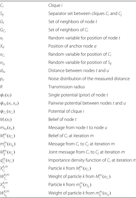
Table 1 Summary of notation
Ci Cliquei
Sij Separator set between cliquesCiandCj
Gt Set of neighbors of nodet
GCi Set of neighbors ofCi
xt Random variable for position of nodet
Xa Position of anchor nodea
xCi Random variable for position ofCi
xSij Random variable for position ofSij
dtu Distance between nodestandu
pv Noise distribution of the measured distance
R Transmission radius
ψt(xt) Single potential (prior) of nodet
ψtu(xt,xu) Pairwise potential between nodestandu
ψCi(xCi) Potential of cliquei
Mt(xt) Belief of nodet
mtu(xu) Message from nodetto nodeu
Mm
i (xCi) Belief ofCiat iterationm mm
ij(xSij) Message fromCitoCjat iterationm Mm
ij(xCj) Joint message fromCitoCjat iterationm qmC
i(xCi) Importance density function ofCiat iterationm XCk,m
i ParticlekfromM
m i (xCi) WCk,m
i Weight of particlekfromM
m i (xCi) XSk,m
ij Particlekfromm
m ij(xSij) WSk,m
graphs, we define aroot node, which is a node without par-ent, andleaf node, which is a node without children. In order to define a graphical model, we place at each node a random variable taking values in some space. Each edge in the graph represents the information about conditional dependency between two connected nodes. In case of cooperative localization, each random variable represents the 2D (or 3D) position, and each edge, which indicates that the measurement is available, represents the likeli-hood function of that measurement. If we exclude the anchors nodes, the graph can be considered as undirected.
2.2 Correctness of belief propagation
In the standard belief propagation (BP) algorithm (also known as sum-product), proposed by Pearl [20], the belief at nodet, which represents the estimate of the posterior marginal PDF, is proportional to the product of the local evidence at that nodeψt(xt), and all the messages coming into nodet:
Mt(xt)∝ψt(xt)
u∈Gt
mut(xt) (1)
wherextis a random variable for the state of nodet(e.g., 2D position), andGtdenotes the neighbors of nodet. The messages are determined by the message update rule:
mut(xt)=
xu
ψu(xu)ψtu(xt,xu)
g∈Gu\t
mgu(xu) (2)
whereψtu(xt,xu)is the pairwise potential between nodes
tandu. On the right-hand side, there is a product over all messages going into node uexcept for the one com-ing from nodet. This product is marginalized in order to form the particular information that we want to send to the destination node. In case of continuous functions, the sum overxuhave to be replaced with the integral.
In practical computation, one starts with nodes at the edge of the graph, and only computes a message when one has available all the messages required. It is easy to see [15] that each message needs to be computed only once for tree-like graphs, meaning that the whole com-putation takes a time proportional to the number of links in the graph, which is significantly less that the exponen-tially large time that would be required to compute the marginal PDFs naively. In other words, BP is a way of orga-nizing the global computation of marginal beliefs in terms of smaller local computations. For the localization prob-lem, this is not sufficient, so we need to represent the messages and beliefs in non-parametric (particle-based) form, as done in [11]. The resulting method, NBP, is capable to approximate the posterior marginal PDFs in non-Gaussian form.
The BP/NBP algorithm does not make a reference to the topology of the graph that it is running on. However,
if we ignore the existence of loops, messages may circu-late indefinitely around these loops, and the process may not converge to a stable equilibrium [20]. One can find examples of loopy graphs, where, for certain parameter values, the BP/NBP algorithm fails to converge or predicts beliefs that are inaccurate. On the other hand, the BP/NBP algorithm could be successful in graphs with loops, e.g., error-correcting codes defined on Tanner graphs that have loops [21].
In order for BP/NBP to be successful, it needs to avoid over-counting[20,22], a situation in which the same evi-dence is passed around the network multiple times and mistaken for new evidence. Of course, this is not the case in tree-like graphs because a node can receive some evidence only through one path. In a loopy network, over-counting could not be avoided. However, BP/NBP could still lead to nearly exact inference if all evidence is over-counted in equal amounts. This could be for-malized byunwrapped network [22] corresponding to a loopy network. The unwrapped network is a tree-like net-work constructed such that performing BP/NBP in the unwrapped network is equivalent to performing BP/NBP in the loopy network. The importance of the unwrapped network is that since it is tree-like, BP/NBP on it is guaran-teed to give the correct beliefs. However, usefulness of this beliefs depends on the similarity between the probability distribution induced by the unwrapped network and the original loopy network. If the distributions are not similar, then the unwrapped network is not useful and the results will be erroneous as in original loopy network.
For the extensive analysis of this problem, we refer the readers to [15,22,23].
2.3 Junction tree formation
if each node, which is in two cliquesCiandCj, is also in all cliques on the unique path betweenCiandCj. If the RIP is not satisfied for one node, there is no theoretical guar-antee that its belief in one clique is the same as its belief in another clique.
We illustrate the whole procedure in Figure 1. We first triangulate the graph by adding the edge between nodes 2 and 5 (Figure 1a). Then we form the cluster graph (Figure 1b) with cliquesCi(t,u,v) and the separator sets
Sij(q,r) (Sij = Ci ∩Cj), where t, u, v are the nodes in
(a)
1(1,2,6) C
2(2,5,6) C
3(2,3,5)
C C4(3,4)
34(3)
S
12(2,6)
S
23(2,5)
S
(d)
1(1,2,6) C
2(2,5,6) C
3(2,3,5)
C C4(3,4)
34(3)
S 13(2)
S
12(2,6)
S
23(2,5)
S
(b)
1(1,2,6) C
2(2,5,6) C
3(2,3,5)
C C4(3,4)
34(3)
S 13(2)
S
23(2,5)
S
(c)
Figure 1Illustration of junction tree formation(a)Triangulated 6-node graph, and corresponding(b)cluster graph,(c)clique tree, and(d)junction tree.
the clique, and q, rare theseparator nodes. Finally, any spanning tree represents the clique tree, such as ones in Figure 1c,d. The tree in Figure 1d is the maximum span-ning tree (|S12| > |S13|), so it represents the JT of the initial graph. Note that the tree in Figure 1c does not satisfy RIP since the node 6, which is inC1andC2, is not inC3.
The described procedure represents the exact forma-tion of JT, also called chordal graph method. The main problem of this approach is the triangulation phase. Find-ing, a minimum triangulation, i.e., one where the largest clique has minimum size, isNP-hard problem due to the number of permutations that must be checked. Of course, there exist an approximate methods (e.g., [25]) which are less expensive, but still too costly according to authors. For more details, see Chapter 10 in [24].
3 PJT
Due to the high complexity of the optimal JT formation, it is necessary to find some approximation that will be suit-able for the cooperative localization problem. Therefore, our goal is to achieve the following.
(a) The number of cliques should be reasonable (i.e., in the order of number of nodes).
(b) In order to reduce the dimensionality of the problem, each clique should include no more than three nodes.
(c) Since the triangulation is expensive procedure, we are going to avoid it, even if it causes the break of RIP for some small percentage of the nodes.
After these approximations, the final result represents, strictly speaking, the clique tree. However, since it is very close to the junction tree (measured by the percentage of the nodes that satisfies RIP), we name it PJT.
3.1 Thin graph formation
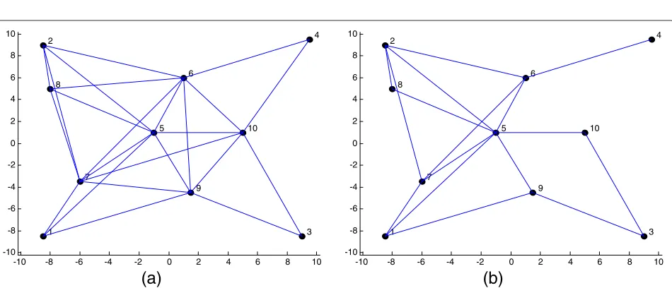
Nevertheless, the spanning tree is very coarse approxi-mation of the original graph since it excludes a lot of edges from the graph. For example, in any spanning tree, one communication failure breaks the graph into two parts. As a consequence, we need more spanning trees in order to have reasonable accurate inference in graphical models. Therefore, we modify standard BFS method by permitting each root node to make an additional visit to the node that was already visited by some of the previous roots. All edges found by first and second visits, along with all the nodes from the original graph, represent the thin graph. In addition, the second visit will automatically form a loop, so we use it to form 3-node clique. The 2-node cliques can be found easily by taking all the edges that appear in thin graph, but not in any 3-node clique. The worst com-plexity isO(v+e+v·(v−1)) ≈ O(v2), since for each of the additional visit, we need to check all previous roots (all the nodes minus one, in the worst case). The detailed pseudocode is shown in Algorithm 1, and an example of the original graph and the corresponding thin graph are shown in Figure 2a,b, respectively.
Algorithm 1. Searching for thin graph and cliques using modified BFS method
1: Input: node listQ and root node root 2: Copy to node lists:Nodes,NewVisit←Q
3: Set current root:r←root
4: Create list of neighbors for all nodesn∈Q:Gn 5: whileNodes is not emptydo
6: for allnodest∈Grdo
7: ift∈Nodesthen
8: Removet from Nodes
9: Insertt in WaitingRoots 10: InsertdrtinT
11: else ifdrt∈/T and r∈NewVisitthen
12: InsertdrtinT
13: Remover from NewVisit 14: Create 3-node cliques:
15: for allq∈PreviousRootsdo
16: if{drq,dtq} ∈Tthen 17: C3nodes← {r,t,q}
18: end if
19: end for
20: end if
21: end for
22: Insertr in PreviousRoots
23: Set current root:r←first unused node from WaitingRoots
24: end while
25: Create 2-node cliquesC2nodes: each edge inT which is not subset ofC3nodes
26: Output: thin graph{Q,T}and cliques
C=C2nodes∪C3nodes
The main benefit of the thin graph is that it mainly includes 3-node loops. The number of these loops, which is obviously always less than the total number of nodes, is nearly constant with respect to connectivity, so the number of cliques will nearly be constant as well. On the other hand, the main drawback is that there exist the loops which include more than three nodes.aThese loops should be triangulated, but we prefer to avoid it in order to keep reasonable complexity. Thus, for n-node loops (n> 3), we form maximumn2-node cliques, using each edge (which is not already subset of any 3-node clique) of the loop as a clique. Another problem can be caused by the nodes which cannot determine their positions due to the possible non-rigidity of the thin graph (e.g., the nodes with less than three neighbors). However, these nodes can be still located since we bounded the estimate within its bounding box (see Section 4.1), created using original (not thin) graph. Therefore, the estimates will never be out
-10 -8 -6 -4 -2 0 2 4 6 8 10 -10
-8 -6 -4 -2 0 2 4 6 8 10
1 2
3 4
5 6
7 8
9
10
(a)
-10 -8 -6 -4 -2 0 2 4 6 8 10 -10
-8 -6 -4 -2 0 2 4 6 8 10
1 2
3 4
5 6
7 8
9
10
(b)
of these boxes, which means that we ensured a coarse estimate in the worst case scenario. Finally, we note that anchor-unknown links are not excluded, so it would be useful if the anchors are placed as close as possible to the edges of the deployment area, where the leaf nodes are expected.
3.2 PJT formation
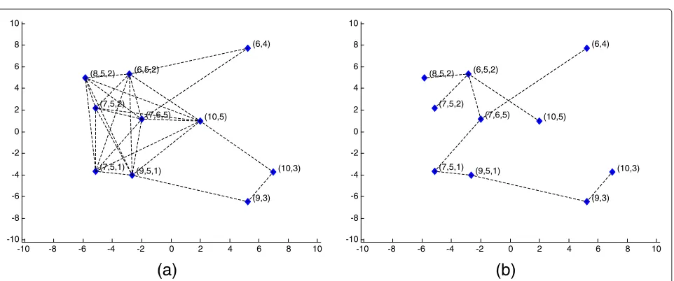
Having defined the cliques, we can form the cluster graph by connecting all pairs of the cliques with non-empty intersection (see Figure 3a). As we already mentioned, the JT, as well as PJT, is the maximum spanning tree of the cluster graph. It can be found using, e.g., Prim’s algorithm [27], as shown in Algorithm 2. The Prim’s algorithm is a method that finds a maximum (or minimum) spanning tree for a connected weighted undirected graph, meaning that the total weight of all the edges in the final tree is max-imized (or minmax-imized). In our case, the algorithm starts with a list (i.e.,CurrentListin Algorithm 2) which initially includes only randomly chosen root clique. At each step, among all the edges between the cliques in the list and those not in the list yet, it chooses the one with the maxi-mum weight and increases the list by adding the explored clique. Finally, it stops when all the cliques are spanned. The example of PJT is shown in Figure 3b. The worst case complexity isO(e·log(v))[27], but in our case the weights are binary (Sij=1, orSij=2), so the execution will be very fast.
Algorithm 2. PJT formation using Prim’s algorithm
1: Input: node listQ and cliques C 2: Create weighted cluster graph: 3: for allpairs{i,j}do
4: Weights(i,j)=Ci∩Cj 5: end for
6: Insert random root clique inCurrentList 7: while|CurrentList|<|C|do
8: Choose edge{m,n}with maximal weight, such thatCmis inCurrentList andCnis not 9: InsertCninCurrentList
10: Insert edge{m,n}inD 11: end while
12: Output: PJT{C,D}
The BP/GBP methods are naturally distributed through the network which means that there is no central unit (fusion center) which will handle all computations. Thus, the proposed PJT formation should be done in a dis-tributed way. It is already well known that there is a straightforward distributed way to form any spanning tree, so we refer the readers to [28,29].
Having defined PJT, it remains to define the communi-cation between neighboring cliques. Since the separator sets, between each pair of the neighboring cliques, are always non-empty, the separator nodes are responsible to perform the communication. Practically, these nodes rep-resents the cluster heads. For example, in Figure 3b, the node 3 will request all the data from node 9, and upon receiving, it will send the data to node 10, and vice versa.
Finally, the previous approximations will likely break the RIP for some small number of the nodes. For instance, in the PJT in Figure 3b, the node 10 (due to the non-triangulated 4-node loop: 3–9–5–10), and the node 7 (due to the appearance of 4-node clique: 2–6–5–7) do not sat-isfy the RIP. Therefore, we do not have a guarantee that the belief of that node in one clique is the same as its belief in another clique [24]. Nevertheless, for coopera-tive localization, this is not a problem since we used the
-10 -8 -6 -4 -2 0 2 4 6 8 10 -10
-8 -6 -4 -2 0 2 4 6 8 10
(10,3) (10,5)
(9,5,1)
(9,3) (8,5,2)
(7,5,1) (7,5,2)
(7,6,5) (6,5,2)
(6,4)
(a)
-10 -8 -6 -4 -2 0 2 4 6 8 10 -10
-8 -6 -4 -2 0 2 4 6 8 10
(10,3) (10,5)
(9,5,1)
(9,3) (8,5,2)
(7,5,1) (7,5,2)
(7,6,5) (6,5,2)
(6,4)
(b)
bounded boxes (see Section 4.1) for the initial set of par-ticles. Regarding other applications, this method might be useful if all edges provide the same (or sufficiently similar) amount of information.
3.3 Possible alternatives
Although we provided a tractable solution for formation of the approximated junction tree, we cannot claim that it is an optimal one. In literature, there are available alterna-tives that could be (with some adaption) applied for this problem. For example, Dechter et al. [30] propose iter-ative join-graph propagation, which runs on the cluster graph with bounded cluster size, created without discard-ing any edges. Similar solution, thin junction tree with bounded cluster size, is available in [31]. However, for both approaches, a distributed implementation is not pro-vided, so they cannot directly be applied for our problem. Finally, it is worth mentioning a distributed method [32], which creates a rigid subgraph from the fully connected (complete) graph in a tractable way. However, this method can be applied for cooperative localization, only if adapted for non-complete graphs.
4 Nonparametric generalized belief propagation GBP-JT is a standard message passing method for the exact inference in graphical models. This can be proved using elimination procedure [18]. Given cliques Ci and its potentialsψCi(xCi), and given the corresponding
junc-tion tree which defines links between the cliques, we send the following message from cliqueCi to cliqueCjby the message update rule:
mij(xSij)=
Ci\Sij
ψCi(xCi)
k∈GCi\j
mki(xSki) (3)
whereSij=Sji=Ci∩Cj, and whereGCiare the neighbors
of cliqueCi(including anchor nodes, which are not part of PJT). The belief at cliqueCiis proportional to the product of the local evidence at that clique and all the messages coming into cliquei:
Mi(xCi)∝ψCi(xCi)
j∈GCi
mji(xSji) (4)
Finally, the single-node beliefs can be obtained via fur-ther marginalization.
Mi(xi)=
Ci\i
Mi(xCi) fori∈Ci (5)
Equations (3), (4), and (5) represent GBP-JT algorithm which is valid for any arbitrary graphs. The standard BP algorithm [11] is a special case of GBP-JT, obtaining by noting that the original tree is already triangulated, and has only pairs of the nodes as cliques. In that case, setsSij are single nodes, and the marginalization is unnecessary.
In order to adapt GBP-JT to iterative scenario for coop-erative localization, Equations (3), (4), at iterationm+1 can be written as
mmij+1(xSij)=
1 mmji(xSji)
Ci\Sij
Mmi (xCi) (6)
Mmi +1(xCi)∝ψCi(xCi)
j∈GCi
mmji+1(xSji) (7)
At the beginning, it is necessary to initializem1
ij=1, and
Mi1= ψCi. The clique potentialψCiis given as a product of all single-node and pairwise potentials. The potentials of 2-node cliqueCi(t,u)and 3-node cliqueCj(t,u,v)are, respectively, given by
ψCi(xCi)=ψtu(xt,xu)ψt(xt)ψu(xu) (8)
ψCj(xCj)=ψtu(xt,xu)ψtv(xt,xv)ψuv(xu,xv)ψt(xt)
×ψu(xu)ψv(xv)
(9)
The single-node potential (the prior) of nodetis given by
ψt(xt)=
1, withinb.box
0, otherwise. (10)
The bounding box (b. box) of node t, created using approximated distances to anchors (only 1-hop and 2-hop) as constraints [33], represents the region of the deployment area where the node t is localized. The pairwise potential ψtu, which represents the likelihood function about the distance between nodes t and u, (ψtu(xt,xu)∝p(dtu|xt,xu)) is given by
ψtu(xt,xu)=pv(dtu− xt−xu) (11) where dtu represents the measured distance between nodestandu,pv(·)the noise distribution of the measured distance, and R the transmission radius. More general model, which incorporates the probability of detection, can be found in [11,33].
Regarding the model for mobile scenario, assuming that information is moving only forward in time, there are no loops between different time frames. Therefore, a dynamic model should be defined on the original graph with nodes. One option is to include this information using single-node potential, i.e.
ψt(xt,τ)=p(xt,τ|xt,τ−1), (12)
where a dynamic model p(xt,τ|xt,τ−1) defines the possi-ble positions of the unknown node xt,τ in current time
on the static scenario. More details on mobile positioning can be found in [13,14,34].
Due to the high complexity, the presence of nonlinear relationships, and potentially highly non-Gaussian uncer-tainties, GBP-JT method is not appropriate for cooper-ative localization [11]. Thus, we need to use NGBP-JT. Moreover, due to the problems explained in previous sections, we are going to use PJT instead of JT. Therefore, in following subsections, we propose NGBP based on PJT (NGBP-PJT) for the arbitrary networks. Note that an anal-ysis of NGBP-JT for the small-scale network has already been provided in [19].
4.1 Drawing particles from the cliques Let us drawNC weighted particles,
WCk,m
i ,X
k,m Ci
(k = 1,. . .,NC,m= 1), from cliquei. Since it is computation-ally very expensive to draw particles from M1i = ψCi,
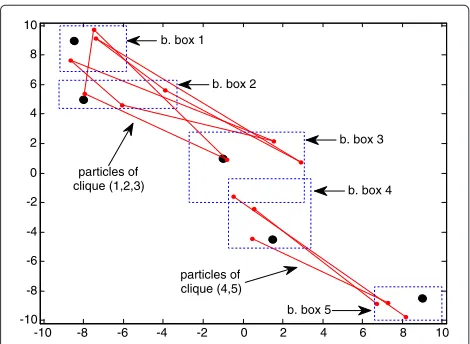
we need to find appropriate importance density function. Thus, for the initial particles, we are going to use two constraints: (i) each particle of the node must be inside its bounding box, and (ii) the distance between each pair of the nodes in clique should be close to the mean value of the measured distance. Taking this into account, our importance density functionqmC
i(m=1) for cliqueCi(t,u)
is given byb:
q1Ci(xCi)=q
1 tu(xt,xu)
=
ψt(xt)ψu(xu), ifμtu− xt−xu)< δ , otherwise
(13)
where μtu is the mean value of measured distance (we assumed that we obtained more measurements per link). The parameter δ should be chosen so as to encompass nearly the whole PDF. Otherwise, if we cut out significant part of the PDF, the final beliefs will be overconfident. For instance, ifpv is a Gaussian with standard deviationσd, δ = 3σd could be a good choice since it will encompass about 99% of the PDF. If the constraint is not satisfied, there is very small probability for the particle in that area.c Finally, it is straightforward to show, using (13), that the importance density function, for 3-node clique Cj(t,u,v), can be found as
q1Cj(xCj)= q1tu(xt,xu)q1tv(xt,xv)q1uv(xu,xv) (14) To draw clique particle, we need to draw node particles within its boxes and accept the particle if the constraint is satisfied. If not, we reject the sample, and try again. The weights of the particles can easily be computed by
WCk,1i =ψCi(X
k,1 Ci)/q
1 Ci(X
k,1
Ci) (15)
Then these weights (as well as all the weights in the following subsections) are normalized
WCk,1i =WCk,1i / k
WCk,1i (16)
In this way, we have created two types of particles: the edges (for 2-node cliques), and the triangles (for 3-node cliques). We illustrated an initial set of particles in Figure 4.
4.2 Computing messages
Having computed the initial set of particles from the beliefs, we can compute the particles from the messages. According to Equation (6), we first need to marginalize the belief from previous iteration, then divide it by the incom-ing message from the previous iteration. Since all node particles within the clique have one common weight (e.g.,
{WCk,im, XCk,im} = {WCk,im, {Xtk,m,Xuk,m}}), we can simply pick the particles of separator nodes (from the clique that send the message), and compute the weight as reminder of (6). The separator sets can include one or two nodes, so there exist 1-node and 2-node messages. Therefore, the weighted particles of the 2-node message fromCi(t,u,v) toCj(t,u,r), at iterationm+1, are given by
XSk,m+1
ij = {X
k,m
t ,Xuk,m} (17)
WSk,m+1
ij =
WCk,m
i
mmji(Xtk,m,Xuk,m)
(18)
The 1-node messages can be found in analog way. As we can see, we need to approximate the parametric form of
-10 -8 -6 -4 -2 0 2 4 6 8 10 -10
-8 -6 -4 -2 0 2 4 6 8 10
particles of clique (1,2,3)
particles of clique (4,5) b. box 1
b. box 2
b. box 3
b. box 4
b. box 5
the messagemmji, so we estimate it using spherically sym-metric Gaussian kernel [12,35]. The bandwidth, parame-ter which controls the smoothness of this kernel density estimate (KDE), can be found using “rule of thumb” [12], or some advanced method [36]. In case of 2-node message, it is too complex to estimate the parametric form directly from high-dimensional (4D) particles. However, thanks to the dependency between the nodes within the message (the noisy distance), we can reduce the dimension of the message by
mmji(xt,xu)=mmji(xt)ψtu(xt,xu)ψu(xu) (19)
Note that in PJT (in contrast to JT), there is always observed distance between each pair of the nodes within the clique (i.e., no additional edges added by triangula-tion). Thus, it is sufficient to transmit the particles over one node, and upon receiving, shift them in a random direction for the observed distance. Finally, the messages from any anchorato any neighboring unknown node t, are simply given in the parametric form
mat(xt)=ψat(Xa,xt) (20)
where we assumed that the position of the anchor node is perfectly known (i.e., defined by Delta Dirac function). However, if anchors’ positions are uncertain (as in [37]), the message can be computed in the same way as the messages from the unknown nodes.
4.3 Computing beliefs
According to (7), the belief of clique i is a product of its clique potential and all the messages coming into the clique. Before drawing the particles, we need to solve two problems: (i) the messages include information about dif-ferent nodes within the clique, and (ii) it is intractable to draw the particles from the product.
The first problem can be solved by filling the message with the information about the nodes which appears in the destination clique, but not in the message. For example, for the messagemmij+1(xt,xu), fromCi(t,u,v)toCj(t,u,r), we can form thejoint message:
Mmij+1(xt,xu,xr)=
mmij+1(xt,xu)ψtr(xt,xr)ψur(xu,xr)ψr(xr)
(21)
Taking Equations (19), (8), and (9) into account, the joint message can be written as
Mmij+1(xCj)=m
m+1
ij (xt)ψCj(xCj) (22)
where nodet must be in appropriate separator set (t ∈ Sij), and if Sij > 1, we can pick one node randomly. Thanks to the particles from the standard messages, we already have few (one or two) node particles from each joint message. The remained node particles can be drawn by shifting given node particles in a random direction for an amount which represents the observed distance, and
by checking (only in case of 3-node clique) another dis-tance constraint. The weights of the particles from the joint messages are equal to the weights of the particles from the standard messages. However, due to the sample depletion, weresample with replacement[38,39] so as to produce the particles with same weights:{1/NC,Xijk,m+1}. The most of the particles, especially in case of small noise, will be the same. This can cause very poor representation of the beliefs. Therefore, to each of these particles, we add a small jitterωdrawn frompv
Xijk,m+1=Xijk,m+1+ω·[ cos(θ ) sin(θ )] (23)
whereθrepresents a random direction (θ ∼Unif[ 0, 2π )). Finally, we solve problem (ii), by making the sum (instead of the product) of the joint messages (i.e., using mix-ture importance sampling(MIS) [11]). Therefore, the final importance density for the belief of cliquej, and corre-sponding particles, are, respectively, given by
qmC+1
j (xCj)=
i∈GCj
Mmij+1(xCj) (24)
{WCk,jm,q+1,XCk,jm,q+1
GCj
k=1 } = { 1
GCj·Nc
, i∈GCj
Xijk,m+1}
(25)
We now find the set of particles from the beliefs
{WCk,jm+1,XCk,jm+1}(k=1,. . .,NC):
XCk,jm+1=choose(XCk,jm,q+1
GCj
k=1) (26)
WCk,jm,corr+1=WCk,jm,q+1
i∈GCj
mmij+1(XkS,m+1
ij )
qmC+1
j (X
k,m+1 Cj )
(27)
WCk,m+1
j =W
k,m+1 Cj,corr·ψCj(X
k,m+1 Cj )
t∈Cj a∈GCj
mat(Xkt,m+1)
(28)
whereWCk,jm,corr+1is the correction of the weights due to the MIS,Xtk,m+1particle from nodet,matis the message from the anchor nodeato unknown nodet, and functionchoose chooses randomly one particle fromGCj.
As a convergence parameter, we use approximated Kullback-Leibler (KL) divergence between the beliefs in two consecutive iterations, which is given by:
KLmj +1=
k
WCk,m+1
j log[W
k,m+1 Cj /M
m
j (XCk,jm+1)]
where we used the approximation Mmj +1(XCk,jm+1) ≈ WCk,m+1
j . The algorithm stops whenKL
m+1
j (for allj) drops below the predefined threshold. However, it is also possi-ble to predefine the number of iterations, given diameter of the graph and transmission radius. We choose the latter approach in simulations.
The final estimation of each node within the cliques is given as the mean of the particles from the belief in last iteration. Since the most of the nodes appear in more than one clique, we simply average multiple estimates. Other options are also possible, such as choosing the belief with the smallest entropy. We summarize the NGBP-PJT algorithm in Algorithm 3.
Algorithm 3. NGBP-PJT method for cooperative localization
1: for allunknown nodesdo
2: Obtain distance measurements to all neighbors 3: Construct the bounded box
4: Set all parameters to the initial values 5: end for
6: Form PJT using Algorithms 1 and 2 7: for allcliquesdo
8: Draw initial particles from the importance density function (13) or (14)
9: form=1 :Niterdo
10: Compute particles for outgoing messages via (17)-(18)
11 Compute (eventual) messages from anchors via (20)
12: Compute KDE of the messages
13: Draw particles from the joint messages (22) 14: Resample with replacement
15: Add small jitter to all particles via (23) 16: Compute particles from the beliefs via
(24)-(28)
17: end for
18: end for
19: Compute final location estimates
Finally, it is worth noting that a special case of NGBP-PJT method is NBP method based on thin graph (NBP-TG) assuming that the thin graph has only the pairs of the nodes as cliques. NBP-TG is very important by-product since it runs on the same graph as NGBP-PJT, which makes this method cheaper than NBP. It also helps to understand (as shown in the following section) how much the removed edges from the original graph affect the performance of the method.
5 Performance evaluation 5.1 Scenario
We assume that there areNa+Nu = 60 nodes in a 20× 20 m2area. Four anchors are placed near the edges. This, usually realistic, constraint helps the unknown nodes near
the edges which suffer from low connectivity. The rest of the anchors and the unknowns are randomly deployed within the area. The number of iterations is set toNiter = 3, which means that each node/clique will have available all the information 3-hop away from itself. The transmis-sion radius is set toR= 8 m. Simulations are performed usingNa = 6 and Na = 12 anchor nodes. We assume that the distance is obtained from RSS measurements using log-normal model, since this is usually the worst case scenario [1]. Thus, we chooseσdB=5 dB as standard deviation of RSS (i.e., the parametersdof log-normal dis-tribution areμ=log(d)andσ =σdB/10np=0.25, where
np = 2 is the path-loss exponent.e). Previous parameters are same both for NBP, NBP-TG, and NGBP-PJT. How-ever, the number of particles is set to 100 (for NBP), 290 (for NBP-TG), and 210 (for NGBP-PJT), in order to make nearly the same computational time for all three methods (see Table 2). For the KDE of the messages, the band-width is found using “rule of thumb”, which is the simplest option. Finally, the following simulation results represent the average over 20 Monte Carlo runs (in each of them, there are Nu estimates available). Note that all defined parameters are valid only if not otherwise stated in the following text.
5.2 Comparison of accuracy and convergence
Using the defined scenario, we compare the accuracy and the convergence of NBP, NBP-TG, and NBP-PJT algo-rithms. The error is defined as Euclidean distance between the true and the estimated location. First, we illustrate the results of these methods in Figure 5. We can see that NBP-PJT method significantly outperforms both NBP and NBP-TG methods, and also that NBP slightly outperforms NBP-TG.
Then, for randomly chosen node, we illustrate its ini-tial and final belief in Figure 6. First, the iniini-tial beliefs of NBP and NBP-TG represent nearly uniform distribution within its bounded box, but the initial belief of NGBP-PJT (which is also within its bounded box) is not uniform due to the distance constraints within appropriate cliques (see (13)). Thus, the initial belief of NGBP-PJT is more infor-mative than the belief of NBP. Second, we can see that the final NBP belief is the tightest, but this information is overconfident comparing with NBP-TG and NGBP-PJT. Since NBP-TG and NGBP-PJT run on the same graph, we can say that NBP-TG is overconfident, comparing
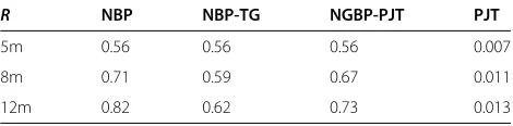
Table 2 Comparison of the computational cost (measured in MFlops)
R NBP NBP-TG NGBP-PJT PJT
5m 0.56 0.56 0.56 0.007
8m 0.71 0.59 0.67 0.011
-10 -8 -6 -4 -2 0 2 4 6 8 10 -10
-8 -6 -4 -2 0 2 4 6 8 10
(a)
-10 -8 -6 -4 -2 0 2 4 6 8 10 -10
-8 -6 -4 -2 0 2 4 6 8 10
(b)
-10 -8 -6 -4 -2 0 2 4 6 8 10 -10
-8 -6 -4 -2 0 2 4 6 8 10
(c)
Figure 5Illustration of results for the 60-node network.(a)NBP,(b)NBP-TG, and(c)NGBP-PJT. The anchors are marked with red squares, the unknowns with black circles, and the estimated locations with black dots.
with NGBP-PJT, due to the loops. Regarding compari-son between NBP and NBP-TG, we note that the latter one has less number of the edges and less number of the loops. This increase the uncertainty, so NBP-TG provides more uncertain belief. The level of overconfidence can be
NBP (initial belief)
−5 0 5
−2 0 2 4 6 8 10
NBP (final belief)
−5 0 5
−2 0 2 4 6 8 10
NBP−TG (initial belief)
−5 0 5
−2 0 2 4 6 8 10
NBP−TG (final belief)
−5 0 5
−2 0 2 4 6 8 10
NGBP (initial belief)
−5 0 5
−2 0 2 4 6 8 10
NGBP (final belief)
−5 0 5
−2 0 2 4 6 8 10
Figure 6Comparison of NBP, NBP-TG and NGBP-PJT beliefs in the first and last iteration.True position of the node is marked withX.
also analyzed using the true position of the node. Hence, in case of overconfident belief, the true position can be located in the area with probability close to zero (as shown in Figure 6). Therefore, we can conclude that NGBP-PJT is less informative, but more trustful. Moreover, in order to obtain more precise conclusion about accuracy, we also consider cumulative distribution function (CDF) of the error in position. We can see in Figure 7 that NGBP-PJT outperforms all other methods in terms of any percentile. Furthermore, we provide the analysis of the RMS error with respect to transmission radius. According to Figure 8, the NGBP-PJT significantly (5–10%) outperforms NBP and NBP-TG, for all R and both values of Na. It is also worth noting that the number of anchors signifi-cantly affects the accuracy. For instance, NGBP-PJT with 6 anchors performs similar as NBP with 12 anchors. There-fore, given nearly the same accuracy, one can decrease the equipment cost by removing 6 anchors (which are usually very expensive). It is also interesting to note the perfor-mance difference between NGBP-PJT and NBP-TG (since they use different message passing, but the same graph),
10 20 30 40 50 60
0 0.1 0.2 0.3 0.4 0.5 0.6 0.7 0.8 0.9 1
error [%R]
CDF
NGBP−PJT − 12 anchors NGBP−PJT − 6 anchors NBP − 12 anchors NBP − 6 anchors NBP−TG − 12 anchors NBP−TG − 6 anchors
5 6 7 8 9 10 11 12 10
20 30 40 50 60 70
Transmission radius [m]
RMS error [%R]
NGBP−PJT − 12 anchors NGBP−PJT − 6 anchors NBP − 12 anchors NBP − 6 anchors NBP−TG − 12 anchors NBP−TG − 6 anchors
Figure 8The effect of transmission radius on RMS error in position.
and the difference between NBP and NBP-TG (since they use the same message passing, but different graph).
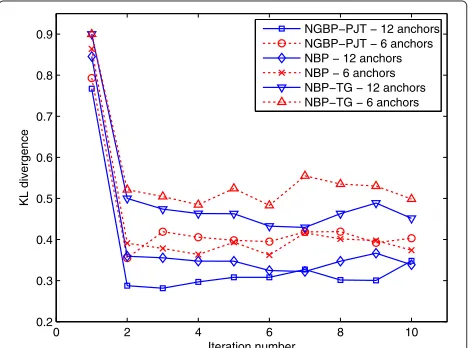
Regarding convergence, we can see in Figure 9 that all algorithms converge sufficiently after second iteration. This is expected since we setR=8 m, so almost all infor-mation is maximum 2-hop away from each clique. Finally, we can see that all algorithms, especially NBP-TG, cannot perfectly converge (i.e.,KL→0) after reasonable number of iterations. This is, of course, caused by the existence of loops (for NBP and NBP-TG), and missing edges in thin graph (for NBP-TG and NGBP-PJT).
5.3 Comparison of computational and communication cost
As we already mentioned, we set the same computational cost forR=5 m by choosing appropriate number of par-ticles for all three methods. It was not possible to set the
0 2 4 6 8 10
0.2 0.3 0.4 0.5 0.6 0.7 0.8 0.9
Iteration number
KL divergence
NGBP−PJT − 12 anchors NGBP−PJT − 6 anchors NBP − 12 anchors NBP − 6 anchors NBP−TG − 12 anchors NBP−TG − 6 anchors
Figure 9Comparison of KL divergence in each iteration.
same cost for all methods since the cost is more sensitive toRin case of NBP method. On the other hand, NGBP-PJT and NBP-TG costs are less sensitive toRdue to the nearly same number of edges with respect to (w.r.t.)R, in formed thin graph. We provide the average cost per node for different values ofRin Table 2. We can see that the cost of NGBP-PJT is the same or less for all considered values ofR. We can also see that the complexity of the PJT formation is neglectable comparing with full algorithms.
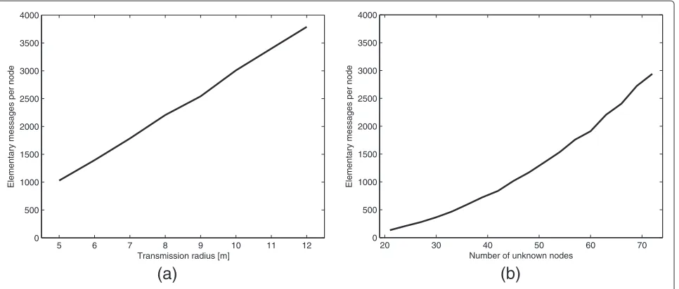
Regarding communication cost, which is directly related with the battery life of the wireless devices, we provide a simplifiedf analysis by counting elementary messages, where one elementary message is defined as a scalar value (e.g., one coordinate of one particle). We will consider the effect of transmission radius and number of unknowns, since their variations obviously affect the cost. First, we analyze the cost of PJT formation (Algorithms 1 and 2). As we can see in Figure 10, it is a linear function of trans-mission radius, and a quadratic function of number of unknowns. Second, we analyze the cost of all considered algorithms w.r.t.R, for two different number of unknowns. According to Figure 11, we can conclude the following
• NGBP-PJT significantly outperforms NBP and NBP-TG methods, for reasonable number of unknowns.
• Comparing with NBP, the improvement of NGBP-PJT is increasing as transmission radius increasing. This is achieved thanks to the thin graph.
• The cost of NBP-TG is slightly less than NGBP-PJT due to the redundancy in PJT graph (i.e., when the same node appears in more than one clique).
• Increasing the number of unknowns will decrease the benefit of NGBP-PJT. This is caused by quadratic dependency of PJT formation w.r.t. number of unknowns. Using results from Figures 10b and 11, we estimate that NGBP-PJT will reach the same cost as NBP, for 140 unknown nodes.
Finally, we can conclude that the proposed NGBP-PJT method is cheaper for reasonably sized networks. How-ever, it can also be cheap for very large-scale networks if the network is divided into regions, and one PJT created for each of them.
5.4 Experimental results
5 6 7 8 9 10 11 12 0
500 1000 1500 2000 2500 3000 3500 4000
Transmission radius [m]
Elementary messages per node
(a)
20 30 40 50 60 70
0 500 1000 1500 2000 2500 3000 3500 4000
Number of unknown nodes
Elementary messages per node
(b)
Figure 10Communication cost for PJT formation w.r.t.(a)transmission radius,(b)number of nodes.
the center frequency 2443 MHz. The measurements are conducted by placing the transmitter and receiver at each pair of the points, and taking 5 measurements for each combination (totally, 9460 measurements). Then, for each measurement, TOA and RSS have been estimated, and for each link, the average has been found. More details about the experiments can be found in [40].
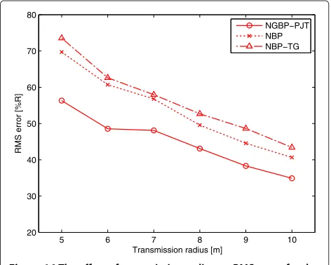
In this article, we use averaged RSS samples, shown in Figure 13. TakingP0(d0 = 1m) = −37 dBm, the param-eters of the log-normal model can be found:np = 2.3 andσdB = 3.92 dB. Then, we compare the accuracy of NGBP-PJT, NBP-TG and NBP as a function of transmis-sion radius (which varies from 5 to 10 m). The number of particles is the same as for the test in Section 5.2, and
5 6 7 8 9 10 11 12
0.5 1 1.5 2 2.5 3 3.5 4 4.5 5 5.5x 10
4
Transmission radius [m]
Elementary messages per node
NBP
NGBP−PJT − 54 unknowns NGBP−PJT − 27 unknowns NBP−TG − 54 unknowns NBP−TG − 27 unknowns
Figure 11The effect of transmission radius on communication cost (for two different number of unknowns).NBP cost is the same for any number of unknowns, so we just plot one curve.
the number of anchors is set toNa = 5 (marked as red squares in Figure 12). The results are averaged over 20 Monte Carlo runs (in each run, we use different seed for the particles, but keep the same network and the corre-sponding measurements). As we can see in Figure 14, the conclusion is the same as for the previous test (Section 5.2) based on synthetic data: NGBP-PJT outperforms NBP and NBP-TG, for all considered R. However, comparing Figures 8 and 14, we note that the values of the errors has changes.
6 Conclusion and future work
In this article, we presented NGBP-PJT, a novel message passing approach for cooperative localization in wire-less networks. Since the exact formation of junction tree
−4 −2 0 2 4 6 8 10
0 2 4 6 8 10 12
Figure 12The deployment of the sensors in a14×13m2
0 2 4 6 8 10 12 14 16 18 −75
−70 −65 −60 −55 −50 −45 −40 −35 −30
distance [m]
RSS [dBm]
Figure 13Obtained measurements (marked with X) and the corresponding log-normal model (black line).
is intractable, we proposed the formation of PJT, which represents the approximated JT based on thin graph. In addition, in order to decrease the number of particles for NGBP-PJT method, we proposed a more informa-tive importance density function, and also reduce the dimensionality of the messages. As by-product, we also proposed NBP-TG, a cheaper variant of NBP, which runs on the same graph as NGBP-PJT. According to our simu-lation and experimental results, NGBP-PJT, outperforms NBP and NBP-TG in terms of accuracy, computational and communication cost in reasonably sized networks. In addition, NGBP-PJT beliefs are not overconfident as NBP beliefs, so we can obtain online more trustful information about the position uncertainty. Finally, all algorithms con-verge sufficiently after very small number of iterations, but the convergence is not perfect.
5 6 7 8 9 10
20 30 40 50 60 70 80
Transmission radius [m]
RMS error [%R]
NGBP−PJT NBP NBP−TG
Figure 14The effect of transmission radius on RMS error, for the network shown in Figure 12, and the measurement model shown in Figure 13.
There remain a number of open directions for the future work. One direction could be to find an alternative method (e.g., modified variants of the methods described in Section 3.3), which will be tractable in large-scale net-works. It would be also useful to find in which graphs, and under which conditions, the benefit gained by using a NGBP-PJT instead of NBP outweighs the penalty caused by discarding edges. Moreover, an important research line is to investigate if there is some cheaper (non-particle-based) message representation, which should be capable to handle all realistic uncertainties. Finally, distributed tar-get tracking in sensor network [42,43] could be an inter-esting direction since this application requires a number of sensor nodes with known (or estimated) positions.
7 Endnotes
aAccording to our empirical analysis, the number of these
loops is relatively small (e.g., just one 4-node loop in Figure 2b).
bWe implicitly assumed thatq1
Ci(xCi) = 0 if the state of
one of the clique nodes is out of the deployment area. cIn practical circumstances, we can set=0.
dNote that these values do not represent the mean value
and the standard deviation of the distance. They are respectively given by:μd = eμ+σ
2/2
,σd = μd
eσ2−
1. Consequently, these parameters are distance dependent. eTypical values forn
p are between 2 and 6 [44]. For the distance estimation, the minimum value is the worst case. fExact communication cost can only be measured by
knowing the hardware specifications, especially, the amount of the bytes in the package, number of re-served bytes in package, energy required to transmit a package, etc.
Competing interests
The authors declare that they have no competing interests.
Acknowledgements
This study was supported in part by the FPU fellowship from Spanish Ministry of Science and Innovation; program CONSOLIDER-INGENIO 2010 under the grant CSD2008-00010 COMONSENS; the European Commission under the grant FP7-ICT-2009-4-248894-WHERE-2; the Swedish Foundation for Strategic Research (SSF) and ELLIIT.
Received: 27 October 2011 Accepted: 17 January 2013 Published: 9 February 2013
References
1. N Patwari, JN Ash, S Kyperountas, AO Hero III, RL Moses, NS Correal, Locating the nodes: cooperative localization in wireless sensor networks. IEEE Signal Process. Mag.22(4), 54–69 (2005)
2. AH Sayed, A Tarighat, N Khajehnouri, Network-based wireless location: challenges faced in developing techniques for accurate wireless location information. IEEE Signal Process. Mag.22(4), 24–40 (2005)
3. D Fox, W Burgard, F Dellaert, S Thrun. Monte Carlo localization: efficient position estimation for mobile robots, inProceedings of the National Conference on Artificial Intelligence, (July 1999)
5. S Gezici, Z Tian, GB Giannakis, H Kobayashi, AF Molisch, HV Poor, Z Sahinoglu, Localization via ultra-wideband radios: a look at positioning aspects for future sensor networks. IEEE Signal Process. Mag.22(4), 70–84 (2005)
6. D Niculescu, B Nath, vol. 5. Ad hoc positioning system (APS), inIEEE Proceedings of the GLOBECOM, (November 2001), pp. 2926–2931 7. Y Shang, W Ruml, Y Zhang, M Fromherz, Localization from connectivity in
sensor networks. IEEE Trans. Parallel Distrib. Syst.15(11), 961–974 (2004) 8. F Chan, HC So, W-K Ma, A novel subspace approach for cooperative
localization in wireless sensor networks Using Range Measurements. IEEE Trans. Signal Process.57(1), 260–269 (2009)
9. A Savvides, H Park, MB Srivastava. The bits and flops of the n-hop multilateration primitive for node localization problems, inProceedings of the 1st ACM International Workshop on Wireless Sensor Networks and Application, (September 2002), pp. 112–121
10. C Pedersen, T Pedersen, BH Fleury. A Variational message passing algorithm for sensor self-localization in wireless networks, inProceedings of the International Symposium on Information Theory (ISIT), (July 2011), pp. 2158-2162
11. AT Ihler, JW Fisher I I I, RL Moses, AS Willsky, Nonparametric belief propagation for self- localization of sensor networks. IEEE J. Sel. Areas Commun.23(4), 809–819 (2005)
12. AT Ihler, Inference in sensor networks: graphical models and particle methods, PhD Thesis. Massachusetts Institute of Technology, June 2005 13. H Wymeersch, J Lien, MZ Win, Cooperative localization in wireless
networks. Proc. IEEE.97(2), 427–450 (2009)
14. J Schiff, EB Sudderth, K Goldberg. Nonparametric belief propagation for distributed tracking of robot networks with noisy inter-distance measurements, inIEEE Proceedings of the International Conference on Intelligent Robots and Systems, (October 2009), pp. 1369–1376 15. JS Yedidia, WT Freeman, Y Weiss, Understanding belief propagation and
its generalizations. Explor. Artif. Intell. New Millennium.8, 239–269 (2003) 16. V Savic, A Poblacion, S Zazo, M Garcia, Indoor positioning using
nonparametric belief propagation based on spanning trees. EURASIP J. Wirel. Commun. Netw.2010, 1–12 (2010)
17. V Savic, H Wymeersch, F Penna, S Zazo. Optimized edge appearance probability for cooperative localization based on tree-reweighted nonparametric belief propagation, inProceedings of the IEEE International Conference on Acoustics, Speech and Signal Processing (ICASSP), (May 2011), pp. 3028–3031
18. MI Jordan, Y Weiss. 2nd edn. Graphical model: probabilistic inference, in
The Handbook of Brain Theory and Neural Networks(MIT Press, Cambridge, MA, p. 2002
19. V Savic, S Zazo. Sensor localization using nonparametric generalized belief propagation in network with loops, inIEEE Proceedings of Information Fusion, (July 2009), pp. 1966–1973
20. J Pearl,Probabilistic Reasoning in Intelligent Systems. Networks of plausible inference. (Morgan Kaufmann, Burlington, MA, 1988)
21. BJ Frey, vol. 10. A revolution: belief propagation in graphs with cycles, in
Proceedings of Advances in Neural Information Processing Systems, (1997), pp. 479–185
22. Y Weiss, Correctness of local probability propagation in graphical models with loops. Neural Comput.12(1), 1–41 (2000)
23. JM Mooij, HJ Kappen, Sufficient conditions for convergence of the sum-product algorithm. IEEE Trans. Inf. Theory.53(12), 4422–4437 (2007) 24. D Koller, N Friedman,Probabilistic Graphical Models: Principles and
Techniques. (MIT Press, MA, 2009)
25. F Hutter, B Ng, R Dearden,Incremental thin junction trees for dynamic Bayesian networks. (Technical Report, Darmstadt University of Technology, 2004). http://citeseerx.ist.psu.edu/viewdoc/summary?doi=10.1.1.9.8661 26. DA Bader, K Madduri. Designing multithreaded algorithms for
breadth-first search and st-connectivity on the Cray MTA-2, inIEEE Proceedings of the Parallel Processing, (August 2006), pp. 523–530 27. X Wang, X Wang, DM Wilkes, A divide-and-conquer approach for
minimum spanning tree-based clustering. IEEE Trans. Knowledge Data Eng.21(7), 945–958 (2009)
28. A Yoo, E Chow, K Henderson, W McLendon, B Hendrickson, UV Catalyurek. A scalable distributed parallel breadth-first search algorithm on Bluegene/L, inProceedings of the Supercomputing, (November 2005) 29. AJ Mooij, N Goga. A distributed spanning tree algorithm for
topology-aware networks, inProceedings of the Conference on Design, Analysis, and Simulation of Distributed Systems, (2004)
30. R Dechter, K Kask, R Mateescu. Iterative join-graph propagation, in
Proceedings of the Conference on Uncertainty in Artificial Intelligence (UAI), (2002)
31. A Chechetka, C Guestrin. Efficient principled learning of thin junction trees, inAdvances in Neural Information Processing Systems (NIPS), (2007) 32. TS Caetano, T Caelli, D Schuurmans, DAC Barone, Graphical models and point pattern matching. IEEE Trans. Pattern Anal. Mach. Intell.28(10), 1646–1663 (2006)
33. V Savic, S Zazo. Nonparametric boxed belief propagation for localization in wireless sensor networks, inIEEE Proceedings of the SENSORCOMM, (June 2009), pp. 520–525
34. L Mihaylova, D Angelova, DR Bull, NC Canagarajah, Localization of mobile nodes in wireless networks with correlated in time measurement noise. IEEE Trans. Mob. Comput.10(1), 44–53 (2011)
35. BW Silverman,Density Estimation for Statistics and Data Analysis. (Chapman and Hall, New York, 1986)
36. ZI Botev,A novel nonparametric density estimator. (Technical Report, The University of Queensland, Australia, 2006)
37. M Vemula, MF Bugallo, PM Djuric, Sensor self-localization with beacon position uncertainty. Signal Process (Elsevier).89(6), 1144–1154 (2009) 38. PM Djuric, JH Kotecha, J Zhang, Y Huang, T Ghirmai, MF Bugallo, J Miguez,
Particle filtering. IEEE Signal Process. Mag.20(5), 19–38 (2003) 39. MS Arulampalam, S Maskell, N Gordon, T Clapp, A tutorial on particle
filters for online nonlinear/non-Gaussian Bayesian tracking. IEEE Trans. Signal Process.50(2), 174–188 (2002)
40. N Patwari, AO Hero, M Perkins, NS Correal, RJ O’Dea, Relative location estimation in wireless sensor networks. IEEE Trans. Signal Process.51(8), 2137–2148 (2003)
41. Wireless Sensor Network Localization Measurement Repository. http:// web.eecs.umich.edu/∼hero/localize/
42. AF Garcia-Fernandez, J Grajal, Asynchronous particle filter for tracking using non-synchronous sensor networks. Signal Process (Elsevier).91(10), 2304–2313 (2011)
43. PM Djuric, J Beaudeau, MF Bugallo. Non-centralized target tracking with mobile agents, inProc. of IEEE Int. Conf. on Acoustics, Speech and Signal Processing (ICASSP), (May 2011), pp. 5928–5931
44. TS Rappaport,Wireless Communications: Principles and Practice, 2nd edn. (Prentice Hall PTR , Upper Saddle River, NJ, 2001)
doi:10.1186/1687-6180-2013-16
Cite this article as:Savic and Zazo:Nonparametric generalized belief prop-agation based on pseudo-junction tree for cooperative localization in wireless networks.EURASIP Journal on Advances in Signal Processing2013 2013:16.
Submit your manuscript to a
journal and benefi t from:
7Convenient online submission
7Rigorous peer review
7Immediate publication on acceptance
7Open access: articles freely available online
7High visibility within the fi eld
7Retaining the copyright to your article