Nonparametric Bayesian Filtering for Location Estimation, Position Tracking, and Global Localization of Mobile Terminals in Outdoor Wireless Environments

(1)

Volume 2008, Article ID 317252,14pages doi:10.1155/2008/317252

Research Article

Nonparametric Bayesian Filtering for Location Estimation,

Position Tracking, and Global Localization of

Mobile Terminals in Outdoor Wireless Environments

Mohamed Khalaf-Allah

Institute of Communications Engineering, Faculty of Electrical Engineering and Information Technology, Leibniz University of Hannover, Appelstrasse 9A, 30167 Hannover, Germany

Correspondence should be addressed to Mohamed Khalaf-Allah,[email protected]

Received 28 February 2007; Revised 16 August 2007; Accepted 10 November 2007

Recommended by Richard J. Barton

The mobile terminal positioning problem is categorized into three diﬀerent types according to the availability of (1) initial accurate

location information and (2) motion measurement data.Location estimationrefers to the mobile positioning problem when both

the initial location and motion measurement data are not available. If both are available, the positioning problem is referred to as

position tracking. When only motion measurements are available, the problem is known asglobal localization. These positioning problems were solved within the Bayesian filtering framework. Filter derivation and implementation algorithms are provided with emphasis on the mapping approach. The radio maps of the experimental area have been created by a 3D deterministic radio propagation tool with a grid resolution of 5 m. Real-world experimentation was conducted in a GSM network deployed in a

semiurban environment in order to investigate the performance of the diﬀerent positioning algorithms.

Copyright © 2008 Mohamed Khalaf-Allah. This is an open access article distributed under the Creative Commons Attribution License, which permits unrestricted use, distribution, and reproduction in any medium, provided the original work is properly cited.

1. INTRODUCTION

Mobile terminal (MT) positioning is a key problem in wire-less environments. It is the most fundamental problem to provide customers with tailored and location-aware services. MT positioning is defined as the determination of the MT ge-olocation using location-dependent parameters in a specific coordinate system. The key driver for developing MT loca-tion technologies in the USA was E-911. In the EU, it was commercial services in the first place, and later E-112 that utilizes the same techniques. Emergency call location has be-come a requirement in fixed and cellular networks in the USA in 1996 [1] and in the EU in 2003 [2]. Positioning of an MT is considered more critical because MT users and hence MT originated emergency calls are continually increasing. It is es-timated that about 50% of all emergency calls in the EU are MT originated, and the expected tendency is rising [2].

The first application of MT location dates back to World War II, when it was critical to locate military personnel rapidly and precisely in emergency situations [3]. Further-more, nonmilitary interest in this field dates back to about 40

years ago [4,5]. While emergency call location could be con-sidered the most important of location-based services (LBSs) due to its urgency for life and property safety, commercial LBSs are believed to make increasing revenues for network operators who could provide customers with attractive and tailored services [6]. Therefore, a lot of research is being car-ried out in this area.

Positioning systems are usually categorized according to the place where location calculations are performed into network-based or mobile-based, or according to the appli-cation environment into outdoor or indoor. The main ap-proaches of positioning are global or satellite-based tech-niques, and local or terrestrial-based methods. Terrestrial-based methods have two variants:geometric techniques, and mapping approaches. These methods diﬀer in terms of ac-curacy, coverage, cost, mobile terminal power consumption, and wireless system impact.

(2)

thus increasing the system impact. The main drawbacks are high-power consumption, need of clear view to at least four satellites (for stand-alone GPS), and the costs of integrat-ing GPS receivers into the MTs. Furthermore, A-GPS solu-tions increase overhead costs due to the requirement to in-stall reference GPS receivers. The satellite-based approach is the most accurate MT positioning technique, and it was only made accessible for commercial applications in the nineties. Also the EU is most likely to follow the US and Japan in re-quiring high-positioning accuracy of mobile emergency calls from 2010 when the Galileo system will be fully operational [7]. However, the benefits of satellite-based positioning could be limited where location information is still needed due to signal blocking. In such cases, other positioning methods should be triggered in order to backup the failed or degraded satellite signals.

Geometric methods estimate the MT location by tri-angulation of, for example, of-arrival (TOA), time-difference-of-arrival (TDOA), enhanced-observed time-difference (EOTD), angle-of-arrival (AOA) measurements, or relationship between received signal strength attenuation and distance to base stations (RSSAD). The main drawback of TOA measurements is the need of mutual synchroniza-tion of the involved base stasynchroniza-tions (BSs) in order to avoid de-graded location accuracy, which is difficult to achieve. Ex-ploiting AOA measurements increases overhead costs due to the need for installation of special antennas at the BSs. At least three BSs are required for TDOA measurements, which cannot always be fulfilled in many situations. RSSAD equa-tions are not really accurate even when using at least three BSs. Although geometric techniques are generally more rate than mapping methods, their position estimation accu-racy degrades severely in multipath environments, which is the dominant condition in built-up areas, and in nonline-of-site (NLOS) situations without accurate environmental in-formation.

Mapping-based mobile location is one way to achieve ac-curacy improvement of cell-ID positioning. They also ap-pear in the literature under the names database compari-sonorcorrelation,location fingerprinting, andpattern recog-nitionormatching. In these techniques, a database, or map of location-dependent parameters, is constructed using ra-dio wave propagation prediction tools [8–10], field mea-surements [11,12], or a combination of both [13]. Later a moving MT collects measurements to be compared with the entries of the database in order to yield location es-timates. Propagation prediction tools are advantageous in terms of cost and map construction time. These tools vary in terms of accuracy according to the degree of geographi-cal information precision integrated in the geographi-calculations, thus are divided into deterministic (3D), semi-deterministic (2– 2.5D), or simple empirical formulas. Field measurements provide more realistic databases but at higher costs and longer construction time that render wide deployment im-practical. Nevertheless field measurements in some parts of the deployment environment do help to show the perfor-mance upper limit of location estimation algorithms us-ing the mappus-ing approach. Location-dependent parameters usually used for mapping include received signal strength

Table1: Phase II of the FCC’s E911 program requirement on loca-tion accuracy.

Network-based Mobile-based

67% 100 m 50 m

95% 300 m 150 m

levels (RxLevs) from surrounding BSs [8–11, 13] and the channel impulse response (CIR) [12, 14, 15] which is the multipath propagation delay profile of the environment. In GSM systems, the bandwidth is too small, unlike the UMTS system, for accurate positioning based on correla-tion of CIR only [12]. Also the geometric time-based (TOA, TDOA, EOTD) and angle-based (AOA) methods could be used as location signatures either stand-alone (less accu-rate) or combined with other location parameters. To the best of the author’s knowledge they are not widely used. However, in [16] a network-based fingerprint method com-posed of TOA and AOA has been procom-posed for wireless lo-cation finding in urban environments, and was found that AOA is more significant than TOA for location discrimina-tion.

Mapping methods often utilize prediction data of RxLev and/or CIR produced during network planning. In the online positioning phase they use only the network available mea-surements and thus they do not require any expensive hard-ware installations at BSs or in MTs. Also they have short de-ployment time and cover current and legacy handsets. This is advantageous in terms of cost, coverage, and system impact compared to the other approaches. Therefore, they seem to be the first alternative to take into consideration, especially for European network operators, since EU mobile location requirement still does not specify any accuracy levels unlike the US mandate, seeTable 1. However, mapping-based solu-tions require continuous update in order to adapt to changes in the environment structure and in the wireless network in-frastructure, and to consider the time-varying nature of wire-less channels.

(3)

Table2: Basic aspects of the diﬀerent positioning techniques.

Accuracy Coverage Cost Terminal power

consumption Wireless system impact

Outdoor Indoor

Global or satellite-based methods

High (∼15 m) Yes None or very poor Medium High Low or medium

Terrestrial geometric techniques

Medium

(∼100 m) Yes Yes Medium Low Medium

Terrestrial mapping approaches

Low

(100 m-several km’s)

Yes Yes Low Low Low

active research topic. A comparison of the basic aspects of the discussed positioning approaches is given inTable 2.

In this paper, a mapping-based method for outdoor wire-less mobile positioning using the Bayesian filtering formu-lation is proposed. Prediction of the average received signal strength at reference locations in a working GSM network is calculated using a 3D radio propagation tool. The motion model of the Bayesian filter utilizes simulated inertial mea-surements. Real-world experiments in a semiurban area have been carried out to study the performance of the proposed techniques.

The rest of the paper is organized as follows.Section 2 defines three diﬀerent positioning problems within the con-text of the mapping approach.Section 3discusses the basics of Bayesian filtering, introduces world model utilized, and gives implementable algorithms for the diﬀerent positioning problems. Experiments and numerical results are presented inSection 4. Finally, the paper is concluded inSection 5.

2. TYPES OF MOBILE TERMINAL POSITIONING PROBLEMS USING THE MAPPING APPROACH

Estimation of the MT position in its environment involves using a map of a location-dependent parameter of the en-vironment, network measurement data, and motion infor-mation. The estimation accuracy could even be enhanced by utilizing any prior knowledge of the MT location when avail-able.

Motion information is generally the most diﬃcult piece of information to extract. Without dedicated motion sen-sors, for example, an inertial measurement unit (IMU), mo-tion estimamo-tion is either impossible or very inaccurate due to the noisy signal behavior used to derive the MT motion pat-tern. Accordingly, the MT positioning problem could be di-vided intolocation estimationandtrackingbased on the avail-ability of motion measurements. Location estimation (LE) algorithms calculate the MT location without incorporat-ing any motion information. Moreover, trackincorporat-ing algorithms could be further categorized according to the availability of prior knowledge into position tracking and global localiza-tion. In position tracking (PT), the initial position of the MT is known, and the problem is to find adequate proce-dures in order to compensate incremental errors in the mo-tion sensor measurements. In the more challenging global

lo-Table3: Comparison of the three positioning problems.

Prior knowledge available?

Motion information

available? Location

estimation No No

Position

tracking Yes Yes

Global

localization No Yes

calization (GL) problem, the initial location of the MT is un-known, and consequently the MT position has to be deter-mined from scratch. This positioning problem is more dif-ficult because multiple and distinct hypotheses have to be handled. The three defined positioning problems are sum-marized inTable 3.

3. BAYESIAN FILTERING FOR MOBILE TERMINAL POSITIONING

3.1. Foundations of the Bayesian filter

and basic algorithm

The recursive Bayesian filter (RBF) [17] is a probabilistic framework for state estimation that utilizes theMarkov as-sumption(i.e., past and future measurements are condition-ally independent if the current state is known). The RBF es-timates the posterior belief of the MT position given its prior belief, motion and network measurements, and the model of the world (or environment).

The prior belief is a probability distribution over all possible locations before taking the MT actions and net-work measurements into account. The posterior belief is the conditional distribution of these locations after incorporat-ing the MT actions and network measurements. The world model is a radio profile map containing predicted received signal strength (RxLev) values at reference locations. The posterior belief distribution is expressed as

Belst

=pst|o0:t,a0:t,m

, (1)

(4)

a0:tare the network measurement data (or network observa-tions) and the actions performed by the MT from time 0 up to timet, respectively, andmis the world model.

ApplyingBayes ruleto (1) we get

Belst

= p

ot|st,o0:t−1,a0:t,m

pst|o0:t−1,a0:t,m

pot|o0:t−1,a0:t,m

.

(2)

Here, actions and network measurements are assumed to oc-cur in an alternative sequence (every action is followed by a network measurement) although in reality they take place concurrently. They are separated only for convenience and clarity of the mathematical treatment.

EmployingMarkov assumptionto the first term in the nominator, and noting that the denominator is a constant probability (denotedη) relative tost, (2) is rewritten as

Belst

=ηpot|st,m

pst|o0:t−1,a0:t,m

. (3)

With the help ofη, which is also callednormalization factor, the resulting product will always sum up to 1. Thus Bel(st) represents a valid probability distribution.

Expanding the right most term in (3) using thetheorem of total probabilitywill result in

Belst

=ηpot|st,m

×

pst|st−1,o0:t−1,a0:t,m

pst−1|o0:t−1,a0:t,m

dst−1. (4)

ApplyingMarkov assumptionto the first term in the inte-gration and noting that the second term is simply Bel(st−1),

we obtain

Belst

=ηpot|st,m p

st|st−1,at,m

Belst−1

dst−1. (5)

Equation (5) is called therecursive Bayesian filter (RBF)and is usually computed in two steps calledpredictionandupdate.

Prediction step:

Bel−st

=

pst|st−1,at,m

Belst−1

dst−1, (6)

where Bel−(st) is the posterior belief just after executing the actionatand before incorporating the network measurement

ot, and p(st |st−1,at−1,m) is the MT motion model, that is,

the transition probability that tells us how the state evolves over time as a function of the MT movements.

Update step:

Belst

=ηpot|st,m

Bel−st

, (7)

where p(ot |st,m) is the network measurement model that specifies the probabilistic law according to which these mea-surements are generated from the state, that is, measure-ments are simply noisy projections of the state [17].

(1) AlgorithmBasic RBF(Bel(st−1),at−1,ot,m)

(2) for allstdo

(3) Bel−(st)=

p(st|st−1,at−1,m) Bel(st−1)dst−1// Prediction

(4) Bel(st)=ηp(ot|st,m) Bel−(st) // Update

(5) endfor

(6) return(Bel(st))

Algorithm1: The basic recursive Bayesian filter algorithm.

Both motion and network measurement models describe the dynamical stochastic system of the MT and its environ-ment. The state at timetis stochastically dependent on the state at timet−1 and the actionat. The network measure-ment ot depends stochastically on the state at timet. Such a temporal model is also known as hidden Markov model (HMM)ordynamic Bayes network (DBN)[17].Algorithm 1 shows a single iteration of the RBF algorithm.

Nonparametric filters (NPFs)[17] provide implementable algorithms for the RBF. They approximate posteriors by a fi-nite number of parameters, each corresponding to a region in the state space, that is, they do not rely on a fixed functional form of the posterior. Moreover, the number of the param-eters used to approximate the posterior can be varied. The quality of approximation depends on the number of these parameters. As the number of parameters approaches infin-ity, NPF tends to converge uniformly to the correct rior. The NPF approach discussed here approximates poste-riors over finite spaces by decomposing the state space into finitely many regions and represents the cumulative poste-rior for each region by a single probability value. Such an ap-proach is known asdiscrete Bayesian filter (DBF). The DBF is also referred to as theforward passof ahidden Markov model. The DBF approximates the belief Bel(s) at any time by a set ofnweighted location candidates as

Bel(s)≈s(i),w(i)i=1:n, (8)

wheres(i) _{= {}_x(i)_,_y(i)_}_{is the}_i_{th MT location candidate (or}

state) andw(i)_{is a probability value (also called}_weight_{) that}

determines the importance of s(i)_{. The sum of all weights}

equals 1 so that Bel(s) represents a valid probability distribu-tion. However, normalization is not a crucial issue for prac-tical algorithm implementation.

3.2. World model

The utilized world model has been constructed by using two input sources. The first are maps of the predicted average received signal strength in a test semiurban area of 9 km2

(5)

5.807 5.8075 5.808 5.8085 5.809 5.8095

×106

Y

(m)

4.343 4.344 4.345 4.346

X(m) ×106

1123 705

1340

938 1134 1144

1793 1361

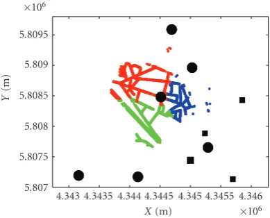
1865

Figure1: Geometry of the base stations in the experimental area. Base stations and indoor antennas are represented by solid circles and squares, respectively.

5.807 5.8075 5.808 5.8085 5.809 5.8095

×106

Y

(m)

4.343 4.344 4.345 4.346

X(m) ×106

Figure2: Locations served by sector cell antennas up to distances

corresponding to TA=0.

involved BSs and distances from the area centric BS to the rest.

After several preprocessing steps as in [19,20], the maps are rearranged so that each raster array contains only the ref-erence locations served by a certain cell antenna. Moreover, each raster array is further divided into smaller arrays ac-cording to timing advance (TA) values; seeFigure 2. This is very useful for the reduction of computational costs. Each ar-ray element containsx-ycoordinates and average predicted RxLev of all involved BSs.

The second input was geographical information system (GIS) data to assist in discriminating between the diﬀerent environmental features, for example, indoor, outdoor, wa-ter, green, and so forth, with very high resolution of 30 cm. Before the arrays that resulted from the preprocessing steps were further divided according to the land feature, which is also very helpful for the computational eﬃciency of the

pro-5.807 5.8075 5.808 5.8085 5.809 5.8095

×106

Y

(m)

4.343 4.3435 4.344 4.3445 4.345 4.3455 4.346

X(m) ×106

Figure3: Outdoor pedestrian locations served by sector cell

anten-nas up to distances corresponding to TA=0.

(1) AlgorithmLocationEstimation(ot,mt)

(2) Bel(st)=0,st=0,mt=DBcell-ID

(3) ot= {cell-IDt, TAt, RxLev(tj)}

(4) fori=1 :ndo

(5) Compute the weightw(ti)

(6) Bel(st)=Bel(st)∪ {s(ti),w(ti)}

(7) endfor

(8) Bel(st)=sort(Bel(st)) // Descending sort

(9) Calculatest

(10) return(st)

Algorithm2: The location estimation algorithm.

posed algorithms, the GIS data resolution was adapted to the 5 m resolution of the radio propagation prediction maps. Figure 3shows outdoor pedestrian locations served by their main sector cell antennas for TA=0. Arrays as depicted in Figure 3were the ones used in the three positioning algo-rithms.

Furthermore, the raster arrays have been re-sampled to 10 m, 15 m,. . ., 50 m resolutions for use only with the loca-tion estimaloca-tion algorithm.

3.3. Location estimation

As mentioned inSection 2the location estimation algorithm calculates the MT position without any prior information about the accurate initial location of the MT or any mo-tion measurements from dedicated sensors. Thus line 3 in Algorithm 1could not be executed. Consequently, the algo-rithm computes only the output probability of the network measurements, which is merely a table-lookup procedure.

(6)

contains location information and expected RxLev values (of the main and neighboring cell antennas) of the areas covered by the main (or serving) cell antenna (or BS) at timet, and RxLev(tj)is the measured received signal strength from thejth observed BS. The weight of the location candidateiis calcu-lated (in line 5) as

w(i)₌_w(i) MM+w

(i) ND+w

(i)

SN, (9)

where wMM(i) , w (i)

ND, and w (i)

SN are the weights according to

themeasurement model,neighborhood degree, andstrongest neighbor,respectively. They are calculated as

wMM(i) =p

ot|s(ti),m

= M

j=1

1

σRxLev√2πe

−(RxLev(tj)−RxLevDBj) 2

/2σ2 RxLev_,

(10)

whereM is the number of observed BSs (main and neigh-boring), that is,Mmax = 7 in typical GSM network mea-surements,σRxLevis the standard deviation of the measured

RxLev, and RxLevDBjis the database RxLev prediction value of thejth observed BS ats(ti):

wND(i) =l, (11)

wherelis the number of observed neighbor BSs that coincide with the list of the predicted six strongest neighbor BSs ats(ti), that is,lmax =6:

w(SNi) =αSN, (12)

whereαSN is a constant bonus value and equals 1. It is as-signed if the strongest observed neighbor BS coincides with the predicted first or second strongest neighbor BS at s(ti). Otherwise,w(SNi) =0.

Intuitively, the summation in (9) should be multiplica-tion. However, summation has two advantages over multipli-cation. First, summation will prevent the assignment of zero to the total weight of any location candidate in case a weight-ing criterion, for example,w(SNi), equals zero. Second,

multi-plication cause many candidates to have very low weights, which will be considered as zero weights if the computer that runs the algorithm has limited numerical precision. Zero weights can cause many problems especially when sorting lo-cation candidates according to their weights. The correct or-der of candidates cannot be determined.

After weight calculation, the location candidate is added to the belief (line 6) together with the assigned weight. This is done for all location candidates before sorting them (line 8) in a descending order with respect to their weights. The aim is not just to find the belief distribution of the MT state, but an estimate of the state calledpoint estimate. This point esti-mate is simply the final MT location estiesti-mate that is output by the algorithm (line 10). There are several ways to calculate point estimates (line 9), for example,maximuma posteriori (MAP),weighted average estimate (WAE), andtrimmed aver-age estimate (TAE).

(1) AlgorithmPositionTracking(st−1,at−1,ot,mt)

(2) st−1=(xt−1,yt−1) // Input

(3) at−1=(transt−1,θt−1) //. . .

(4) ot= {cell-IDt, TAt} //. . .

(5) mt=DBcell-IDt = xj,yj,wj //. . .

(6) x−

t =xt−1+ transt−1·cosθt−1 // Prediction

(7) y−

t =yt−1+ transt−1·sinθt−1 //. . .

(8) for j=1 :ndo // Update

(9) wj=1/

(xt−−xj)2+ (y−t −yj)2

(10)endfor

(11) mt=sort(mt) // Descending sort

(12) st=(xt,yt)=(x1,y1)

(13)return(st)

Algorithm3: The position tracking algorithm.

Maximuma posteriori is simply the location candidate with the highest assigned weight and is expressed as

st=arg max Bel

st

. (13)

If many candidates have the same weight, the returned lo-cation estimate will depend on the stability of the sorting scheme. Stable sorting algorithms maintain the relative order of the location candidates, that is, a location candidate with the highest weight that appeared first in the unsorted belief will also appear first in the sorted belief. This is very disad-vantageous as an arbitrary candidate could be returned as the location estimate though other candidates also assigned with the same highest weight would be more accurate. How-ever, this negative aspect could be reduced by computing the weighted averageof all candidates representing the posterior belief distribution. Thus the location estimate would be

st=

1

n

i=1w(i)

n

i=1

s(ti)×w(i). (14)

The WAE is themean valueof the updated belief distribution and it will coincide with the MAP estimate only forunimodal andsymmetricdistributions, which is not often the case. The trimmed average estimatecalculates the MT location as the average of thekbest weighted candidates as follows:

st=1

k

i=1

s(ti), (15)

wherek < nandnis the total number of location candidates.

3.4. Position tracking

A single iteration of the position tracking algorithm is given in Algorithm 3. The inputs are the initial position (line 2) st−1 = (xt−1,yt−1), the IMU data (line 3) at−1 =

(transt−1,θt−1), where transt−1 andθt−1 are the translation

(7)

(line 5), wherewjis the weight of thejth location candidate and initially set to zero. Note that the proposed algorithm updates only one position hypothesis, that is,nin expression (8) equals 1.

The position tracking algorithm propagates the known initial MT location st−1 using IMU data in the prediction

step (lines 6 and 7). The propagated location is then updated by matching it to the set of candidate locations (lines 8–10) that are covered by the current serving cell antenna, after de-scending sort of the candidates with respect to weight (line 11), the new MT position (line 12) is simply the candidate of the minimum Euclidean distance to the location computed in the prediction step.

3.5. Global localization

The global localization algorithm has no information about the accurate MT position at the beginning. Thus, it has to resolve the location ambiguity and converge to the true po-sition of the MT by tracking all probable location candi-dates and determine their weights every time the algorithm is run. When this task is successfully fulfilled, the algorithm is allowed to run in the position tracking mode (line 30 in Algorithm 4).

As depicted inAlgorithm 4, the global localization algo-rithm is initialized by setting the travelled distance as mea-sured by the IMU (trvld dist) to 0, andModealso to 0, that is, global localization mode (line 3). The inputs (lines 4–7) are the same as inAlgorithm 3except (line 5) that the global localization algorithm tracks a number of hypothetical can-didates, unlike the position tracking algorithm. The global localization mode will run as long as the number of loca-tion candidatesnin the belief distribution Bel(st−1) is greater

than a certain threshold α(line 9). During this mode, the prediction and update steps will only run if the MT’s trav-elled distance is greater than or equal to the database (or map) resolution DBres (line 11), in order to allow position

state transition using the world model. The updated candi-date will only be added to the new belief, if the location it is matched to is not greater than DBres away (lines 19–21).

Therefore, the number of location candidates will decrease after every run of the algorithm until their total number is equal to or less than the thresholdα. In this very event, the updated MT position is simply estimated as the average of the remaining candidates, and the algorithm is switched to the position tracking mode (lines 25–28). Note that the al-gorithm returns no position estimates in the global local-ization mode. First after switching to the position tracking mode, location estimates are returned at the end of every up-date run, seeAlgorithm 3. For both global localization and position tracking algorithms only the cell-ID and TA but no RxLev values of the network measurement report have been utilized, see line 4 inAlgorithm 3and line 7 inAlgorithm 4, respectively.

The update step of the position tracking and global local-ization algorithms has diﬀerent roles. In the position tracking algorithm, the position estimate is decided upon the result of the update step, where in the global localization algorithm, the update step works to reduce the size of the position belief

1: AlgorithmGlobalLocalization(Bel(st−1),at−1,ot,mt)

2: // Initialization, only at the first run of the algorithm

3: trvld dist=0, Mode=0

4: // Inputs

5: Bel(st−1)=DBcell-IDt = xi,yi,i=1,. . .,n

6:mt=DBcell IDt= xj,yj,wj, j=1,. . .,q,wj =0

7:ot= {cell-IDt, TAt},at−1=(transt−1,θt−1)

8:ifMode=0 // Global localization mode

9: if n > α

10: trvld dist=trvld dist

+

(transt−1·cosθt−1)2+ (transt−1·sinθt−1)2

11: if trvld dist≥DBres

12: fori=1 :ndo

13: x−i =xi+ trvld dist·cosθt−1// Prediction

14: yi−=yi+ trvld dist·sinθt−1//. . .

15: for j=1 :qdo

16: wj=1/

(xi−−xj)2+ (yi−−yj)2// Update

17: endfor

18: wj =sort(wj) // Descending sort

19: if (1/w1≤DBres)

20: add (x1,y1) to Bel(st)

21: endif

22: endfor

23: trvld dist=0

24: endif

25: else if n≤α

26: Mode=1

27: st=(ixi/n,iyi/n)

28: endif

29: else ifMode=1 // Position tracking mode 30: PositionTracking(st−1,at−1,ot,mt) //Algorithm 3 31:endif

Algorithm4: The global localization algorithm.

and makes it converge to a single estimate before allowing the position tracking algorithm to run.

3.6. How global localization works

(8)

5.8076 5.8078 5.808 5.8082 5.8084 5.8086

×106

Y

(m)

4.3436 4.3438 4.344 4.3442 4.3444 4.3446 4.3448

X(m) ×106

(a)

5.8076 5.8078 5.808 5.8082 5.8084 5.8086

×106

Y

(m)

4.3436 4.3438 4.344 4.3442 4.3444 4.3446 4.3448

X(m) ×106

(b)

5.8076 5.8078 5.808 5.8082 5.8084 5.8086

×106

Y

(m)

4.3436 4.3438 4.344 4.3442 4.3444 4.3446 4.3448

X(m) ×106

(c)

5.8076 5.8078 5.808 5.8082 5.8084 5.8086

×106

Y

(m)

4.3436 4.3438 4.344 4.3442 4.3444 4.3446 4.3448

X(m) ×106

(d)

5.8076 5.8078 5.808 5.8082 5.8084 5.8086

×106

Y

(m)

4.3436 4.3438 4.344 4.3442 4.3444 4.3446 4.3448

X(m) ×106

(e)

Figure4: Global localization of a mobile terminal in a GSM environment.

4. EXPERIMENTS AND NUMERICAL RESULTS

4.1. Experimental setup

Measurements have been carried out in an E-Plus GSM 1800 MHz network by a pedestrian along a route of about 1940 m long in a 9 km2 _{semiurban environment in}

Han-nover, Germany. There are six BSs, each with three sectors, and four indoor antennas in the test area. RxLev measure-ments of the serving BSs and up to six neighboring stations along with GPS position fixes for ground truth have been

(9)

160 180 200 220 240 260 280 300 320

P

o

sitioning

er

ro

r

(m)

5 10 15 20 25 30 35 40 45 50

Mapping resolution (m) MAP

WAE TAE

Mean positioning error

Figure5: Mean positioning error of the location estimation algo-rithm.

global localization algorithms depend only on the TA mea-surements that correspond to the serving BS wireless cover-age, which can be sufficiently determined offline, taking ac-count of power management effects. Thus, both algorithms are not affected by power management operations. For the location estimation algorithm, the network operator would need to keep prediction information for all possible range of the power management scheme in order to avoid the decrease in accuracy performance.

4.2. Location estimation results

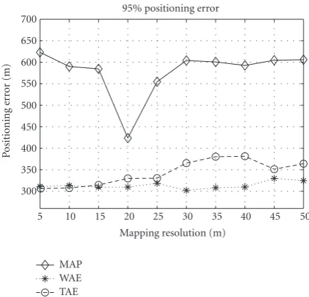
The positioning accuracy of the location estimation algo-rithm has been investigated for the three presented point es-timators and using diﬀerent mapping resolutions. Figures5– 7show the mean, 67 percentile and 95 percentile position-ing error, respectively, of the diﬀerent point estimators with varying world model resolution.

It can be seen that WAE and TAE always outperform the MAP estimator. This is logical as both WAE and TAE con-sider more location candidates of the posterior belief and not only one candidate as the MAP estimator. Because in the context of mobile terminal positioning using RxLev map-ping, multimodal posterior belief distributions are gener-ated; MAP estimation will choose only one peak of the pos-teriors which is not a suitable estimation decision. On the contrary, WAE and TAE consider more than the one peak and thus can better represent the multimodal property of the posterior distributions.

Figure 6also shows that TAE outperforms WAE at the 67 percentile positioning error for all mapping resolution. This might be due to the fact that WAE represents the whole posterior belief distribution, while TAE considers only the upper areas of the posteriors, that is, location

candi-150 200 250 300 350 400 450

P

o

sitioning

er

ro

r

(m)

5 10 15 20 25 30 35 40 45 50

WAE TAE

67% positioning error

Figure6: Sixty-seven percentile positioning error of the location estimation algorithm.

300 350 400 450 500 550 600 650 700

P

o

sitioning

er

ro

r

(m)

5 10 15 20 25 30 35 40 45 50

WAE TAE

95% positioning error

Figure7: Ninety-five percentile positioning error of the location estimation algorithm.

(10)

160 165 170 175 180 185 190 195 200

P

o

sitioning

er

ro

r

(m)

5 10 15 20 25 30 35 40 45 50

Mapping resolution (m) WAE

TAE 10% TAE 20%

TAE 30% TAE 40% TAE 50% Mean positioning error

Figure8: Mean positioning error of the location estimation

algo-rithm using WAE and TAE (k=0.1∗n–0.5∗n).

180 190 200 210 220 230 240 250 260 270 280

P

o

sitioning

er

ro

r

(m)

5 10 15 20 25 30 35 40 45 50

TAE 10% TAE 20%

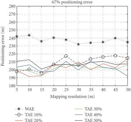
TAE 30% TAE 40% TAE 50% 67% positioning error

Figure9: Sixty-seven percentile positioning error of the location

estimation algorithm using WAE and TAE (k=0.1∗n–0.5∗n).

The explanation is that for lower mapping resolution, considering only upper areas of the posterior belief distribu-tions to calculate a point estimate, as the TAE, will not cor-rectly keep the information represented by the posterior dis-tributions, and thus considering the whole distribution area, as the WAE, is more representative.

In Figures5,6, and7, TAE was calculated by averaging the best 10% weighted location candidates, that is,k=0.1∗n

in (15). The explanation in the previous paragraph can be confirmed if we look at the results obtained whenk is in-creased up to 0.9∗n.

260 280 300 320 340 360 380 420 400

P

o

sitioning

er

ro

r

(m)

5 10 15 20 25 30 35 40 45 50

TAE 10% TAE 20%

Figure10: Ninety-five percentile positioning error of the location

160 165 170 175 180 185 190 195 200 205 210

P

o

sitioning

er

ro

r

(m)

5 10 15 20 25 30 35 40 45 50

TAE 10% TAE 60%

TAE 70% TAE 80% TAE 90% Mean positioning error

Figure11: Mean positioning error of the location estimation

algo-rithm using WAE and TAE (k=0.6∗n–0.9∗n).

Figures8and9show that increasing the number of loca-tion candidates to average (k=0.2∗n–0.5∗n) for TAE with decreasing mapping resolution enhances the performance of TAE at the mean and 67 percentile errors and always out-performs the WAE. We can notice the same tendency in Figure 10. However,khad to be over 0.2∗nin order to out-perform the WAE at the 95 percentile positioning error with decreasing mapping resolution.

(11)

180 190 200 210 220 230 240 250 260 270 280

P

o

sitioning

er

ro

r

(m)

5 10 15 20 25 30 35 40 45 50

TAE 10% TAE 60%

Figure12: Sixty-seven percentile positioning error of the location

260 280 300 320 340 360 380 420 400

P

o

sitioning

er

ro

r

(m)

5 10 15 20 25 30 35 40 45 50

TAE 10% TAE 60%

Figure13: Ninety-five percentile positioning error of the location

WAE forkover 0.8∗n. Also at 67 percentile positioning error inFigure 12no TAE enhancement was achieved by increasing

k. However, at the 95 percentile inFigure 13TAE performed better tillkreached 0.7∗n.

From the previous discussion we can conclude that TAE performs better with lower resolution mapping, that is, up to 15 m, whenkis increased up to 0.5∗n.

We can also generally notice that for all point estimation methods, there is no significant decrease in the positioning accuracy with decreasing mapping resolution. This shall be further investigated by comparing these results with a lower bound, for example, the Barankin bound [21] in a future

0 5 10 15 20 25

Ex

ecution

time

(ms)

5 10 15 20 25 30 35 40 45 50

Mapping resolution (m)

Figure14: The average execution time needed for a single iteration

of the location estimation algorithm using diﬀerent mapping

reso-lutions on a standard PC with 2.2 GHz processor.

work. However, according to this notice it was of interest to calculate how the run time of the location estimation algo-rithm changes with varying mapping resolution.Figure 14 depicts the average computation time needed for a single iteration on a standard PC with 2.2 GHz processor. At the 5 m resolution the execution time was only 23 milliseconds. Computation time then drops down exponentially to under 3 milliseconds as the mapping resolution decreases. However, execution time is linearly proportional to the number of lo-cation candidates.

These results can even suggest providing mobile-based implementation for the location estimation algorithm, which will supply customers with position information for low ac-curacy applications at very low costs. World models can ini-tially be installed in the mobile terminals and updated as needed.

4.3. Position tracking results

Within position tracking experiments the initial location of the MT is known. We have investigated the performance of the tracking algorithm by varyingσtrans from 1% to 10% of the performed translation andσorientbetween 1◦and 6◦. The quality of performance is determined according toreliability andpositioning errorsin meters. We consider the MT position is reliably tracked if the final position estimate error over the whole experiment route of 1940 m is not greater than 50 m. All experiments have been repeated 100 times in order to get reasonable results. It can be seen inFigure 15, as expected, that the higherσtrans and/or σorient are the lower the

relia-bility of the tracking algorithm along the test route. How-ever, forσtransup to 4% andσorientup to 2◦, reliability is over 90% of all repeats. Withσorientup to 2◦andσtransup to 10%,

slightly less than 70% of the cases are successfully tracked. Whenσorientis increased up to 5◦, reliability is at least 60% of

all repeats even with the worst case ofσtrans. Forσorientequals

(12)

80 70 60 50 40 30 20 10 0 90 100

R

eliabilit

y

(%)

1 2 3 4 5 6 7 8 9 10

SD of translation error (%) SD of orientation error=1◦

SD of orientation error=2◦ SD of orientation error=3◦

SD of orientation error=4◦ SD of orientation error=5◦ SD of orientation error=6◦

Figure15: Reliability of position tracking with varying standard deviation (SD) of IMU translation and orientation.

19 18 17 16 15 14 20

M

ean

positioning

er

ro

r

(m)

1 2 3 4 5 6 7 8 9 10

Figure16: Mean position tracking error.

Figure 16shows that the mean positioning error for the diﬀerent cases is between 15 m and 20 m. This is accurate enough for most positioning applications and confirms the suitability of IMU employment for reliable position track-ing. The 67 percentile positioning error is always less than 20 m for all cases as illustrated inFigure 17.Figure 18depicts the 95 percentile position tracking error which is almost al-ways between 52 m and 56 m and less than 62 m in the worst cases.

4.4. Global localization results

In the global localization experiments, the reliability for the diﬀerent values of σtrans and σorient has been investigated.

Global localization is considered reliable, that is,

success-19 18 17 16 15 14 13 20

67%

positioning

er

ro

r

(m)

1 2 3 4 5 6 7 8 9 10

Figure17: Sixty-seven percentile position tracking error.

60 59 58 57 56 55 54 53 61 62

52

95%

positioning

er

ro

r

(m)

1 2 3 4 5 6 7 8 9 10

Figure18: Ninety-five percentile position tracking errors.

ful if the MT position estimation error just before switch-ing to position trackswitch-ing mode (line 30 in Algorithm 4) is not greater than 50 m in order to also allow reliable position tracking. As shown inFigure 19, the global localization relia-bility is over 80% and 65% forσorientup to 3◦and 6◦, respec-tively.

The eﬀect ofσtranson the results is almost not significant,

because of the 5 m map resolution that makes the update step insensitive to the range of translation errors assumed. Moreover, there is a slight tendency to increase the reliability of global localization with increasing σtrans especially when

σorient also increases, which seems counter intuitive.

How-ever, the fact is that large errors caused by highσorientvalues

(13)

90 85 80 75 70 65 60 55 50 95 100

R

eliabilit

y

(%)

1 2 3 4 5 6 7 8 9 10

Figure19: Reliability of global localization with varying standard deviation (SD) of IMU translation and orientation.

5. CONCLUSIONS AND FUTURE WORK

In this paper, the mobile terminal positioning problem was first classified into three types according to the availability of (1) prior knowledge about the accurate initial position of the MT and (2) motion measurement data. Solutions for the three positioning problems have been suggested within the Bayesian filtering framework. Also implementation algo-rithms have been provided and the world model has been de-scribed. Finally, experimental results in a live GSM network have been presented and discussed. The paper showed that reliable accurate position information can be obtained and maintained for mobile terminal users by combining environ-ment radio maps with IMU data.

As mentioned inSection 4.2, calculation of a theoretical lower bound, for example, Barankin bound, on the location estimation performance will be a topic for future work. Also increasing the reliability of the position tracking and global localization algorithms is a possible extension of the work. This shall be achieved by further analysis of the behavior of the algorithms when they incorrectly estimate the MT posi-tion. Results should help develop mechanisms to recognize and handle such situations. It is apparent that the proposed algorithms could be applied in indoor environments as well as for vehicle navigation applications.

ACKNOWLEDGMENTS

This work has been conducted under the supervision of Pro-fessor Kyamakya. The help of many parties was essential. The author would like to thank the Institute for Communications Technology at Braunschweig Technical University and E-Plus Mobilfunk GmbH & CO KG in D¨usseldorf, Germany, for providing the network and radio prediction data. The author is also grateful to the Institute of Cartography and

Geoinfor-matics at the Leibniz University of Hannover for supplying the GIS data utilized in this research.

REFERENCES

[1] Federal Communications Commission (FCC) Fact Sheet, “FCC Wireless 911 Requirements,” 2001.

[2] EU Institutions Press Release, “Commission Pushes for Rapid Deployment of Location Enhanced 112 Emergency Services,” DN: IP/03/1122, Brussels, Belgium, July 2003.

[3] K. Pahlavan and A. H. Levesque,Wireless Information

Net-works, John Wiley & Sons, Hoboken, NJ, USA, 2nd edition, 2005.

[4] W. G. Figel, N. H. Shepherd, and W. F. Trammell, “Vehicle

lo-cation by a signal attenuation method,”IEEE Transactions on

Vehicular Technology, vol. 18, no. 3, pp. 105–109, 1969. [5] G. D. Ott, “Vehicle location in cellular mobile radio systems,”

IEEE Transactions on Vehicular Technology, vol. 26, no. 1, pp. 43–46, 1977.

[6] T. M. Rantalainen, M. A. Spirito, and V. Ruutu, “Evolution

of location services in GSM and UMTS networks,” in

Pro-ceedings of the 3rd International Symposium on Wireless Per-sonal Multimedia Communications (WPMC ’00), pp. 1027– 1032, Bangkok, Thailand, November 2000.

[7] Berg Insight, “GPS and Galileo in Mobile Handsets,” Re-search Report, Berg Insight, Gothenburg, Stockholm, Sweden, November 2006.

[8] H. Schmitz, M. Kuipers, K. Majewski, and P. Stadelmeyer, “A new method for positioning of mobile users by comparing a time series of measured reception power levels with

predic-tions,” inProceedings of the 57th IEEE SemiannualVehicular

Technology Conference (VTC ’03), vol. 3, pp. 1993–1997, Jeju, Korea, April 2003.

[9] D. Zimmermann, J. Baumann, M. Layh, F. Landstorfer, R. Hoppe, and G. Wolfle, “Database correlation for positioning of mobile terminals in cellular networks using wave

propaga-tion models,” inProceedings of the 60th IEEE Vehicular

Technol-ogy Conference (VTC ’04), vol. 7, pp. 4682–4686, Los Angeles, Calif, USA, September 2004.

[10] M. Khalaf-Allah and K. Kyamakya, “Database correlation us-ing bayes filter for mobile terminal localization in GSM

sub-urban environments,” inProceedings of the 63rd IEEE

Vehicu-lar Technology Conference (VTC ’06), vol. 2, pp. 798–802, Mel-bourne, Australia, May 2006.

[11] H. Laitinen, J. Lahteenmaki, and T. Nordstrom, “Database

cor-relation method for GSM location,” inProceedings of the 53rd

IEEE Vehicular Technology Conference (VTC ’01), vol. 4, pp. 2504–2508, Rhodes, Greece, May 2001.

[12] T. Nypan, “Mobile terminal positioning based on database comparison and filtering,” Dissertation, Norwegian University of Science and Technology, Trondheim, Norweg, 2004. [13] J. Zhu, “Indoor/outdoor location of cellular handsets based

on received signal strength,” Technical Specification PG-TR-060515-JZ, School of Electrical and Computer Engineering, Georgia Institute of Technology, Atlanta, Ga, USA, August 2006.

[14] M. Layh, U. Reiser, D. Zimmermann, and F. Landstorfer, “Po-sitioning of mobile terminals based on feature extraction from

channel impulse responses,” inProceedings of the 63rd IEEE

(14)

[15] S. Ahonen and H. Laitinen, “Database correlation method

for UMTS location,” inProceedings of the 57th IEEE Vehicular

Technology Conference (VTC ’03), vol. 4, pp. 2696–2700, Jeju, Korea, April 2003.

[16] I. Kelly, D. Hai, and L. Hao, “On the feasibility of the mul-tipath fingerprint method for location finding in urban

en-vironments,”Applied Computational Electromagnetics Society

Journal, vol. 15, no. 3, p. 232, 2000.

[17] S. Thrun, W. Burgard, and D. Fox,Probabilistic Robotics, MIT

Press, Cambridge, Mass, USA, 2005.

[18] T. Kurner and A. Meier, “Prediction of outdoor and

outdoor-to-indoor coverage in urban areas at 1.8 GHz,”IEEE Journal on

Selected Areas on Communications, vol. 20, no. 3, pp. 496–506, 2002.

[19] M. Khalaf-Allah and K. Kyamakya, “Mobile location in GSM networks using database correlation with bayesian

estima-tion,” inProceedings of the 11th IEEE International Symposium

on Computers and Communications (ISCC ’06), pp. 289–293, Cagliari, Italy, June 2006.

[20] M. Khalaf-Allah and K. Kyamakya, “Bayesian mobile

loca-tion in cellular networks,” inProceedings of the 14th European

Signal Processing Conference (EUSIPCO ’06), Florence, Italy, September 2006.

[21] H. Koorapaty, “Barankin bounds for position estimation using

received signal strength measurements,” inProceedings of the