Volume 2006, Article ID 51306, Pages1–11 DOI 10.1155/ASP/2006/51306
Learning-Based Nonparametric Image Super-Resolution
Shyamsundar Rajaram,1Mithun Das Gupta,2Nemanja Petrovic,3and Thomas S. Huang2
1Beckman Institute, University of Illinois at Urbana-Champaign, IL 61801, USA 2Beckman Institute, at Urbana-Champaign, University of Illinois Urbana, IL 61801, USA 3Siemens Corporate Research, Princeton, NJ 08540-6632, USA
Received 1 December 2004; Revised 19 April 2005; Accepted 25 April 2005
We present a novel learning-based framework for zooming and recognizing images of digits obtained from vehicle registration plates, which have been blurred using an unknown kernel. We model the image as an undirected graphical model over image patches in which the compatibility functions are represented as nonparametric kernel densities. The crucial feature of this work is an iterative loop that alternates between super-resolution and restoration stages. A machine-learning-based framework has been used for restoration which also models spatial zooming. Image segmentation is done by a column-variance estimation-based “dissection” algorithm. Initially, the compatibility functions are learned by nonparametric kernel density estimation, using random samples from the training data. Next, we solve the inference problem by using an extended version of the nonparametric belief propagation algorithm, in which we introduce the notion of partial messages. Finally, we recognize the super-resolved and restored images. The resulting confidence scores are used to sample from the training set to better learn the compatibility functions.
Copyright © 2006 Hindawi Publishing Corporation. All rights reserved.
1. INTRODUCTION
Restoration plays a major role in most vision-based systems as the inputs in most cases are blurred/noisy. Blurred images are a nightmare for any recognition system. Many segmenta-tion algorithms fail when the image is badly blurred. Restora-tion is a neat showcase of the ill-posedness of computer vi-sion problems. Given a blurred image, there can be more than one sharp natural image which, when blurred, will gen-erate the original image. In several important applications like surveillance, tracking, and license plate recognition sys-tems, images may be severely blurred. Hence, the recognition strongly depends on the restoration performed either as an independent step or jointly with some other computer vision or learning tasks. In this paper, we present a method which can handle image restoration with super-resolution. Super-resolution is a specific process where the output image is of higher spatial resolution than the input image.
From a restoration point of view, a reasonable estimate of the restored image may be obtained if we have a priori knowledge about the blurring kernel. If no additive noise is present, then Wiener filtering can be used as it is the opti-mal filter. In the presence of additive noise the Weiner filter method gives the mean square error (MSE) minimized solu-tion. In [1], Bascle et al. showed that restoration can be made relatively easy if multiple images are taken into account. Fur-ther, image restoration can be thought of as a special case
of super-resolution. Image deblurring and super-resolution have been treated concurrently by many authors, so we will intermittently (and erroneously) use the terms “sharp” and “high resolution” synonymously.
natural images up to a zoom factor of 8. Along the same lines, Bishop et al. [9] performed video super-resolution by considering additional priors to account for the temporal consistencies between the successive frames. The learning-based methods can be made more powerful and robust if the images are restricted to be of a specific type, as in [8, 13] where face images are hallucinated. In [8], Baker and Kanade proposed a hallucination technique based on the recognition of generic local features. The local features are then used to predict a recognition-based prior rather than a smoothness prior as is the case with most iterative techniques. However, we notice that hallucinated images need not be realistic. The spirit of our work [14] is in close synchronization with the work of Freeman et al., how-ever it differs from [11] in using partial message passing and restoration-recognition loop.
The two unique features of our work are partial mes-sages and the restoration-super-resolution-recognition loop. Restoration is the key block since without restoration, the other modules lack the robustness and accuracy which any vision-based system working with real-life images requires. Our restoration algorithm is built on the notion ofpartial message propagationwherein we propose that any given im-age patch is only partially influenced by its neighbors, de-pending on the spatial orientation. Moreover the difference in sizes of the observed and inferred image patches results in spatial zooming or super-resolution. The model allows us to infer a zoomed version of the original blurred low-resolution image. The recognition step is performed inside the loop as it helps in localization of search space. For example, the search space for an image of the digit “8” can be greatly min-imized if we can introduce information which reduces the search space to the set{0, 3, 6, 8, 9}, which is 50% minimiza-tion from the actual search space 0–9. With subsequent iter-ations, the search space is further reduced until only images of the digit “8” are remaining. Further, our method is not an example-based method, which means that the reconstructed image is not limited to one of the candidates from the train-ing set. It removes the restriction of [11] that reconstructed high-resolution image must be a candidate from the training set whose low-resolution version is the most similar to the input low-resolution patch. Since our method is a learning-based method, the basic assumption is that we have seen the kinds of blurs in the training set which we want to restore in our test cases. In other words, if the training set has ex-amples of Gaussian blurs only, then this set is not adequate for learning potentials when the test cases have motion blur as the primary blur. However, we can combine the training data sets comprising of examples of different kinds of blurs and then use the combined training set to learn the potentials to handle a wide range of blurs in the test cases. We employ sampling techniques to approximate the message products and only partial messages are propagated based on the spatial alignment of the image patches. To target a real-life applica-tion, we develop a fully automated license plate recognition system.
The organization of this paper is as follows. InSection 2, we describe the image model and review the details of the
yc yd
xc xd
ya yb
xa xb
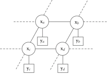
Figure 1: Image model.xi’s are the nonoverlapping hidden im-age patches andyi’s are the observed patches. The potential func-tionsψ(xi,xj) model the interactions between spatial neighbors and
φ(xi,yj) model the association between a patch and its observation.
nonparametric belief propagation (NBP) algorithm. In Sec-tion 3, we present our framework for image segmentaSec-tion and then elaborate our method for restoration, super-res-olution, and recognition in a loop. We introduce the features and potential functions and describe the application of NBP algorithm for restoration and super-resolution. InSection 4, we present experimental results of super-resolution and rec-ognition on synthetic digit images and license plate images. We conclude inSection 5, with a discussion about our work and directions for future research.
2. THE MODEL
2.1. Problem statement and notation
Consider a training set of pairs of images of sizengiven by
{(X1,Y1), (X2,Y2),. . ., (Xn,Yn)}. Let there be an unknown
kernel f (Xi) that maps fromXito Yi. The objective of the
learning algorithm is, given the training set, to learn a model which can be used to infer the imageXfrom an observed im-ageYwhich is not present in the training set. We model the imageXas an undirected graphical model or more specifi-cally a Markov random field (MRF) [11]. MRF is a factorable distribution defined by the graphG = {V,E}where each node represents a random variablexi,i ∈[1· · ·N],
corre-sponding to a patch in the unknown, sharp image, which is associated with an observation nodeyiwhich represents the
corresponding patch in the observed image (Figure 1). An edge between nodexiand nodexjindicates that they are
spa-tial neighbors. The interaction between neighboring patches xiandxjis modelled using a potential function represented
asψ(xi,xj) and commonly called the interaction potential.
The association between the image patchxiand its observed
blurred versionyiis modelled as a pairwise potential
repre-sented byφ(xi,yi)–called the association potential. The
prob-ability distribution over the particular image and its blurred observation p(X,Y) can now be expressed in a factorized form as
p(X,Y)= 1
Z
{i,j}∈E
ψxi,xj i∈V
φxi,yi
Learning with an MRF involves two phases, namely, the learning and the inference phase. In the learning phase, the potentials that model the interactions and associations are learned from the training data. The inference phase com-putes the marginals of posterior distributionp(xi|Y), for all
the nodes i ∈ V. In the next few sections, we review the BP algorithm that will be used in the restoration part of our restoration-recognition loop.
2.2. Belief propagation
For acyclic graphs, the conditional distributions can be cal-culated exactly by a local message-passing algorithm known as belief propagation (BP) [15]. The message propagated from nodeito a node j in thenth iteration represented as
mn
i j(xj) is given by
mni j xj =α xi
ψxi,xj
φxi,yi h∈Γ(i)\j
mn−1
hi
xi
, (2)
whereΓ(i) indicates the neighborhood of the nodexiandα
represents an arbitrary proportionality constant. The mes-sages computed can be combined to obtain the beliefs
bi
xi
=αφxi,yi h∈Γ(i)
mn hi xi . (3)
For tree structured graphs, the beliefs converge to the ac-tual marginal distributions once the messages from each node have been propagated to every other node. Therefore, marginalsp(xi|Y) are given by
pxi|Y
=αφxi,yi h∈Γ(i)
mnhi
xi
. (4)
In the case of graphs with cycles, the BP algorithm is not ex-act. The iterative version of BP algorithm produces the be-liefs which do not converge to true marginals. But it was empirically shown that loopy BP produces excellent results for several hard problems. Recently, Yedidia et al. [16] estab-lished the link between the fixed points of BP algorithm and stationary points of “variational free energy” defined on the graphical model. This important result sheds more light on convergence and optimality properties of loopy BP approxi-mation.
Loopy BP cannot be discretely applied to our model since the messages computed using (2) are mixtures of Gaussians and computing a message mni j(xj) involves the product of
the interaction potentialψ(xi,xj), the association potential
φ(xj,yj), and the messagesmn−1
hi (xi)h∈Γ(i)\jwhere each
term is a mixture of Gaussians. Hence, in order to evaluate (2), the mixture components in the potentials and the mes-sages have to be pruned so that the number of components in the product is within tractable limits to solve the inte-gral (Figure 2). Such an approximation is unsuitable for the restoration problem and alternatively, we use the nonpara-metric extension of belief propagation proposed by Sudderth et al. [17] and independently invented by Isard [18], which we briefly review next. For the next section, we assume that
Figure2: The individual Gaussians in the product can be approxi-mated by fewer Gaussians.
we know the form of the association and interaction poten-tials. The form of the messages as well as the potentials are essentially the same so that the product term can be evalu-ated. Details about learning the potentials are discussed in Section 3.
2.3. Nonparametric belief propagation
We note that the interaction potential can be decomposed into a marginal influence term given byξ(xi) :=
xjψ(xi,xj) and a conditional interaction termψ(xj | xi). The message
update (2) can be written as
mni j xj =α xi
ψxi|xj
πn
i,j
xi
, (5)
πn
i,j
xi
:=φxi,yi
ξxi h∈Γ(i)\j
mnhi−1
xi
. (6)
The modified message update (5) can be solved in two phases. The first phase involves computing the termπni,j(xi)
and the second phase involves integrating the combination ofπn
i,j(xi) with the conditional interaction termψ(xj|xi). In
[17,18], Gibbs sampling technique was used to solve the first phase and the second phase was handled using stochastic in-tegration. The messages were represented nonparametrically using kernel density estimate as
mi j xj = M
m=1
wm
jN
xj;μmj,Λmj
, (7)
where,wm
j,μmj,Λmj correspond to the weight, mean, and
co-variance associated with themth kernel. In the following sec-tions, we will elaborate on the procedure to obtain the mes-sage updates.
2.3.1. Products of Gaussians
Consider the product ofLGaussian distributions,Ll=1N(z;
μl,Λl). The meanμand covarianceΛof the resulting
prod-uct, which is a GaussianN(z;μ,Λ), are
Λ−1=L
l=1
Λ−1
l ,
μ=ΛL
l=1
Λ−1
l μl.
2.3.2. Products of Gaussians with different dimensions
As an introduction to our partial message-passing algorithm, let us consider the product ofLGaussian distributions where the firstL−1 of them are distributions over the random vec-torzof dimensiondand theLth one is a distribution over a subset of the components of the random vectorzof
dimen-siond < d. Without loss of generality, let us consider the case
whenzcorresponds to the firstdcomponents ofz. The re-sulting product of suchLdistributions is a Gaussian, whose meanμand covarianceΛcan be computed in closed form, and is given by
Λ−1=L− 1
l=1
Λ−1
l +
Λ−1
L
d×d (0)d×(d−d) (0)(d−d)×d (0)(d−d)×(d−d)
,
Λ−1μ=L− 1
l=1
Λ−1
l μl
+
Λ−1
L
d×d (0)d×(d−d) (0)(d−d)×d (0)(d−d)×(d−d)
μLd×1
(0)(d−d)×1
.
(9)
The above approach can be extended to handle products of
LGaussian distributions, where each term is a distribution over a different subsetxof the components ofx, where the sets satisfy the property that each component of the random vectorxappears in at least one of theLdifferent sets.
2.3.3. Parallel sampling
The first phase of computing the messages corresponds to evaluating the productπni,j(xi). We observe that each term
in the product is a mixture of Gaussians and, for instance, if each term hasMmixture components, then the product is a mixture ofMLGaussians whereLis the number of terms.
Exact computation of the product can be performed as ex-plained inSection 2.3.1, however, it is not feasible because of the O(ML) computations. Pruning of the mixture
com-ponents can be performed to restrict the number of compu-tations, but it turns out to be a very coarse approximation for the restoration problem. Sequential Gibbs sampling [19] and importance weighting were used in [17,18] to generate
Masymptotically unbiased samples without explicitly com-puting the product.
In this work, we use alternating Gibbs sampling [20] to obtain samples from the productπni,j(xi). The procedure for
alternating Gibbs sampling to sample from a product of the formLl=1
M
m=1wl,mN(z;μl,m,Λl,m) is as follows.
(1) Pick a data vectorzrandomly.
(2) Compute the posterior probability Pl,m = wl,mN(z;
μl,m,Λl,m) for each of theM mixture components in
every term of the product, given the data vectorz. (3) Pick a mixture component ml for each term in the
product based on the posterior probability distribu-tion.
(4) Compute the resulting distribution obtained by mul-tiplying the picked mixture components, that is,
L
l=1N(z;μl,ml,Λl,ml), using (8).
(5) Sample from this resulting distribution to obtain the new data vectorz.
(6) Go back to step 2.
The above technique can be used to obtain asymptoti-cally unbiased samplesx1
i,x2i,. . .,xiM fromπni,j(xi). Further,
the same sampling approach can be used to obtain samples for the posteriorp(xi|Y) given by (4) after each iteration of
the message passing algorithm.
2.3.4. Message updates
The second phase of obtaining the message update is to in-tegrate the combination of the samples obtained from alter-nating Gibbs sampling and the conditional interaction po-tential. This is performed using stochastic integration, where every samplexmi is propagated to nodejby samplingxmj from
ψ(xi=xim,xj). Now, nonparametric density estimation (7) is
used to obtain the messagesmn
i,j(xj), where the means of the
kernels are the propagated samples. Covariances are chosen to be diagonal and identical and are obtained using leave-one outcross validation [21].
3. LICENSE PLATE RECOGNITION (LPR) SYSTEM: AN APPLICATION FOR SEGMENTATION, SUPER-RESOLUTION, AND RECOGNITION
In this section, we will elaborate the algorithmic modules of the entire LPR system. Segmentation is performed outside the loop. First, we elaborate the algorithm for segmenting out images of digits from clustered license plates. For image segmentation, we use a dissection method to cut out the im-ages of the digits from the blurred license plates. Then we will elaborate the application of the NBP algorithm for superre-solving and restoring a blurred and downsampled image of a digit. The recognition phase is explained thereafter, which is the last module in the loop.
From our modeling perspective, the observationY corre-sponds to a blurred and downsampled version of the original imageX with an unknown blurring kernel function f(X). The training set comprises of several instances of image and blurred-downsampled version pairs{X,Y}. As elaborated in Section 2.1,Xis modelled as an MRF over the patch-based representationxi,i∈ [1· · ·N]. The choice of patch size is
often a critical issue, as a small sized patch does not cap-ture enough information which makes the restoration very ill-posed and a bigger sized patch captures too much infor-mation thereby resulting in computational problems. In this work, after performing several experiments, we chose the ob-servation patches to be of size 4×4 and the patches in high-resolution images to be of size 8×8.
3.1. Unsupervised image segmentation
(a)
0 50 100 150 200 250 300 350 400 450 500 0
200 400 600 800 1000 1200 1400 1600
(b)
(c)
(d)
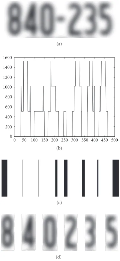
Figure3: (a) blurred input image, (b) variance along a given col-umn, (c) the thresholded variance plot, (d) segmented digits.
always dark and the background is of a lighter shade. Next we assume that the smallest rectangular box binding the dig-its in a plate has the maximum area compared to all other contents of the plate. The segmentation scheme is illustrated in Figure 3. The variance along a column is estimated and then compared against a threshold to obtain the thresholded variance plot inFigure 3. The final segmentation is done by cutting the initial blurred image along the black regions as shown in the fourth image inFigure 3.
3.2. Learning the association and interaction potentials
One of the novelties of this work is in usingnonparametric kernel density estimation for learning the potentialsto avoid
the averaging effects in the parametric methods which is against the spirit of a restoration problem. Namely, one could try to fit the high-resolution portion of the training set with continuous parametric distribution that is tractable for BP algorithm (mixture of Gaussians, e.g.). From a generative model perspective, sampling from such parametric distribu-tion would produce samples that are averaged versions of the images in the training set, and hence the generated images would be blurred. A parametric model would not generate samples that are similar to the training data and hence, we use a nonparametric modeling approach for restoration.
We model the association potentialφ(xi,yi) as a function
over the vectorized patch association, as shown inFigure 4, and with the form
φxi,yi
= 1
M
M
m=1
Nxi,yi t
;μm,Λm
, (10)
whereMis the number of components andN([x,y]t;μ,Λ)
is the multivariate normal distribution with meanμand co-varianceΛover the random vector [x,y]t. From the training
images, the patch association vectors [x,y]t corresponding
to the image and its blurred-downsampled version are con-structed. The patch association vectors are pruned to avoid redundancy. In other words, patches that are similar to each other are represented by a single patch. The potential is con-structed by considering a kernel with the mean chosen as the patch association vector and the covariances are chosen us-ing the leave-one outcross validation technique [21]. The in-teraction potentialψ(xi,xj) is a function over the vectorized two pixel-thick nonoverlapping patch boundary, as shown in Figure 5, and learned using the above mentioned nonpara-metric estimation technique. The interaction potential is of the form
ψxi,xj
= 1
N
N
n=1
Nxj,xi t
;μn,Λn
, (11)
whereNis the number of components andN([xj,xi]t;μ,Λ)
is the multivariate normal distribution with meanμand co-variance Λ over the random vector [xj,xi]t. The notation
xi has been used to denote the boundary pixels which
ac-tually interact while passing messages between two neigh-boring nodes. In our partial message-passing algorithm, only the pixels which are close to the boundary interact with the neighbor as shown inFigure 5. The interaction potential vec-tors are pruned to avoid redundancy just as in the case of the association potential.
yi
xi
4 8 12 16 3 7 11 15 2 6 10 14 1 5 9 13
8 16 24 32 40 48 56 64 7 15 23 31 39 47 55 63 6 14 22 30 38 46 54 62 5 13 21 29 37 45 53 61 4 12 20 28 36 44 52 60 3 11 19 27 35 43 51 59 2 10 18 26 34 42 50 58 1 9 17 25 33 41 49 57
p16
. . .
p2 p1 p64
. . .
p2 p1
yi xi
Figure4: The vectorized pixels in patchxiare appended onto the vectorized pixels in patchyito obtain a feature vector. The association potentialφ(xi,yi) is a function over this feature vector.
xi xj
8 16 24 32 40 48 56 64 7 15 23 31 39 47 55 63 6 14 22 30 38 46 54 62 5 13 21 29 37 45 53 61 4 12 20 28 36 44 52 60 3 11 19 27 35 43 51 59 2 10 18 26 34 42 50 58 1 9 17 25 33 41 49 57
8 16 24 32 40 48 56 64 7 15 23 31 39 47 55 63 6 14 22 30 38 46 54 62 5 13 21 29 37 45 53 61 4 12 20 28 36 44 52 60 3 11 19 27 35 43 51 59 2 10 18 26 34 42 50 58 1 9 17 25 33 41 49 57
p64
. . .
p34 p33 p32
. . .
p2 p1
xi xj
Figure5: The vectorized boundary pixels of patchesxiandxjare appended to obtain a feature vector. The interaction potentialψ(xi,xj) is a function over this feature vector.
functions. The recognition approach is further elaborated in Section 3.4. During the first iteration, the association as well as the interaction potentials are learnt from patches obtained from a randomly sampled set of images in the training set. The learning-based method enables us to restore and hence super-resolve a test image even if we have not seenexactlythe same image in the training ensemble. If a priori knowledge was available about the digit present in the image, then we can learn the potentials only from images of the same digit class. Since we do not have this information, we go for ran-dom training set where each digit is present at least once. By iterating the confidence, the true digit increases and so we se-lect more and more training images from the true digit class. Optimality is ensured in the sense that a particular digit is more or less the same across different font families, provided other factors like size are held constant.
3.3. Restoration and super-resolution using nonparametric belief propagation
The first step in restoration involves iterating the message-passing algorithm several times after which the posterior dis-tribution p(xi|Y),i∈[1· · ·N], can be obtained using
al-ternating Gibbs sampling.
As mentioned earlier, the message updatemn
i,j(xj) is
per-formed in two different phases, where the first phase in-volves sampling from the product πin,j(xi), as in (6),
us-ing the alternatus-ing Gibbs samplus-ing method and the second
Training
data Sampler
Learning association
and interaction
potential Confidence
scores
Recognition Restoration and
super-resolution Blurred image
Figure6: Block diagram illustrating our framework for performing recognition and restoration in a loop.
phase corresponds to stochastic integration by propagating the samples obtained from sampling to node j based on the conditional interaction, which is followed by non para-metric estimation of the message as a kernel density esti-mate. Now, we note that the messagemi,j(xj) is a function
8 16 24 32 40 48 56 64 7 15 23 31 39 47 55 63 6 14 22 30 38 46 54 62 5 13 21 29 37 45 53 61 4 12 20 28 36 44 52 60 3 11 19 27 35 43 51 59 2 10 18 26 34 42 50 58 1 9 17 25 33 41 49 57
8 16 24 32 40 48 56 64 7 15 23 31 39 47 55 63 6 14 22 30 38 46 54 62 5 13 21 29 37 45 53 61 4 12 20 28 36 44 52 60 3 11 19 27 35 43 51 59 2 10 18 26 34 42 50 58 1 9 17 25 33 41 49 57 8 16 24 32 40 48 56 64 7 15 23 31 39 47 55 63 6 14 22 30 38 46 54 62 5 13 21 29 37 45 53 61 4 12 20 28 36 44 52 60 3 11 19 27 35 43 51 59 2 10 18 26 34 42 50 58 1 9 17 25 33 41 49 57 8 16 24 32 40 48 56 64 7 15 23 31 39 47 55 63 6 14 22 30 38 46 54 62 5 13 21 29 37 45 53 61 4 12 20 28 36 44 52 60 3 11 19 27 35 43 51 59 2 10 18 26 34 42 50 58 1 9 17 25 33 41 49 57
8 16 24 32 40 48 56 64 7 15 23 31 39 47 55 63 6 14 22 30 38 46 54 62 5 13 21 29 37 45 53 61 4 12 20 28 36 44 52 60 3 11 19 27 35 43 51 59 2 10 18 26 34 42 50 58 1 9 17 25 33 41 49 57 8 16 24 32 40 48 56 64
7 15 23 31 39 47 55 63 6 14 22 30 38 46 54 62 5 13 21 29 37 45 53 61 4 12 20 28 36 44 52 60 3 11 19 27 35 43 51 59 2 10 18 26 34 42 50 58 1 9 17 25 33 41 49 57
Figure7: Illustration of our partial influence model: pixels 1–32 of the central patch are influenced by pixels 33–64 of the left patch.
the four pixel-thick boundary of the patches corresponding to nodes iand j and further, the messages are denoted as
mn
i,j(xi,j). The alternating Gibbs sampling procedure can still
be used to generate samples fromπn
i,j(xi) with a modification
to step 4 of the algorithm. In the restoration problem setup, the product in step 4 corresponds to
Nxi;μ,Λ
φ(xi,yi)
Nxi,j;μi,j,Λi,j
ξ(x)
h∈Γ(i)\j
Nxh,i;μh,i,Λh,i
mn−1 h,i (xh,i)
,
(12)
where the function indicated under the braces (φ(xi,yi),ξ(x),
ormn−1
h,i (xh,i)) is the term inπin,j(xi) from which the
compo-nent was picked. Except for the first term which is a normal overxi, the rest—the component from the marginal
influ-ence term and the component from the messages—are nor-mal distributions over subsets of the components of the ran-dom vectorxi. Such a product of Gaussians can be solved
using the method discussed in Section 2.3.1 for comput-ing the products of normal distributions over different sub-sets of the components of a random vector. The rest of the alternating Gibbs sampling procedure remains unchanged and can be used to generate samples fromπn
i,j(xi) and
fur-ther these samples are propagated to node jas explained in Section 2.3.4. Several iterations of the message update algo-rithm are performed for all the nodes in the graph and at the end of each iteration, the posteriorp(xi|Y) given in (4)
can be computed using the alternating Gibbs sampling pro-cedure.
One of the key contributions of this framework is han-dling restoration and super-resolution within the same step. Since we learn the interactions between the downsampled
and blurred image patches and their corresponding high-resolution, sharp image patches, we handle both the in-ference problems, namely deblurring and super-resolution, within the same model. In other words, this method extends the learning-based algorithms which have been used by nu-merous researchers in restoration as well as super-resolution.
3.4. Recognition
One of the key contributions of this work is the iterative loop which alternates between restoration/super-resolution and recognition as shown inFigure 6. This feedback feature allows us to perform sampling from the training set in a way which ensures that the data used for learning the potentials are similar to the test data. This technique resembles a boost-ing procedure wherein the distribution over the class labels is modified in order to boost the performance of the restora-tion method.
The algorithm used for recognition of the digits is based on thek-nearest-neighbor algorithm. The Euclidean distance metric is used to compute the distances between the test im-ageXand the images in the database. Based on the distance, the topkclosest points from the dataset{X1,X2,. . .,Xk}are
picked. Let us denote the distances corresponding to the top
kpoints to be{D1,D2,. . .,Dk}and denote the class index of
theith closest image to beci,ci∈[0· · ·9]. Now, we arrive at
a confidence estimate for each class using
C(class=c|X)= 1 Z
k i=1exp
−DiIc
ci
iIc
ci
, (13)
function. The decision rule for recognition is given by
c∗=arg maxcCclass=c|X. (14)
The confidence estimate obtained for each class is a multi-nomial distribution over the class labels. Samples are then generated from the training data set based on this multino-mial distribution and these samples are then used to learn the association and interaction potentials.
4. EXPERIMENTS AND RESULTS
For this work we performed several experiments on synthetic images of digits and actual license plate images. For the high-resolution training data set, we used digit fonts from 20 dif-ferent font families. The digits are represented by same-size center-aligned binary images. The low-resolution training data set consists of corresponding gray-scale images obtained by convolution with a blurring kernel followed by downsam-pling. Different types of blurring kernels used in this work are Gaussian and Laplacian Kernels. Another neat feature of this work is the fact that different types of blurs can be mod-eled simultaneously and inference can be performed in an unified framework. Since we have some idea about the tar-get domain, we can train our algorithm to handle such blur-ring kernels. More severe levels of blur and different types, namely, motion blur, can also be incorporated in this frame-work.
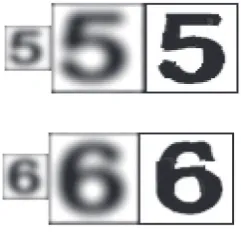
The real data set consists of blurred binary registration plate images. The registration plates are segmented using the algorithm discussed in Section 3.1. To evaluate the results of the restoration algorithm, we subjectively inspect the vi-sual quality of the restored images. The spatial zoom has been fixed to a factor of 2 in both directions. Zoom factors less than 2 can be easily achieved, but for higher zooming levels, the patch sizes for the sharp images have to be very large and hence block effects would start appearing in the in-ferred high-resolution image. Additionally, we measure the improvement in the recognition rate and recognition confi-dence after performing restoration and recognition in a loop. In the first experiment, we perform a “sanity check” to determine the restoration performance for a test image, where the potentials are learned using images from the train-ing set which correspond to the digit in the test image. In Figure 8, we illustrate the restoration of blurred digits “5” and “6.” The reconstructed high-resolution images were al-most indistinguishable from the originals (for digit “5”) or very close to the original (for digit “6”). The zoom factor is 2 in both directions.
In the second experiment, we trained the potentials on a set of 150 synthetic images consisting of 15 images for each digit. The testing set consists of 50 images consisting of 5 im-ages for each digit. We inspected the improvement of visual quality of reconstructed images after each of five iterations of NBP algorithm (Figure 9). We note that the vertical and hor-izontal lines of digit “5” become thinner and clearer as the iterations proceed. For the digit “9,” the reconstruction be-comes less spiky and the semicircular regions become thin-ner and smoother.
Figure8: Left image is the input to the system. Center image is sharpened using deconvolution methods and then zoomed using interpolation methods. Right image is the output of our algorithm. Testing samples are taken from the training ensemble.
Figure9: Restoration result obtained after second, third, fourth, and fifth iterations of the NBP algorithm for “5” and “9.” Zooming factor is equal to 2.
(a) (b)
Figure10: Segmentation results for original license plates: (a) orig-inal plates, (b) segmented digits.
The segmentation routine is tested on actual license plates as shown in theFigure 10. In spite of the very simple segmentation algorithm, the results were near optimum for most cases. In some cases the digits are a little thinner than necessary, but this can be overcome by appropriate padding with the boundary pixels. The individual digit images are resized before they are input to the restoration/super-reso-lution recognition loop.
0 1 2 3 4 5 6 7 8 9 Digits
0 0.1 0.2 0.3 0.4 0.5 0.6 0.7 0.8 0.9
C
o
nfidenc
e
sc
o
re
Original Restored
Figure 11: Confidence scores versus digits. Original confidence scores denote the recognition confidence for the blurred digits, the darker bars show the recognition confidence for restored digits.
this experiment, the training set consists of 200 synthetic im-ages and the test set is composed of 200 real imim-ages from the blurred license plates. We present results of recognition accuracy and the improvement in confidence scores (before and after restoration) after 5 runs of the restoration/super-resolution and recognition loop. There was a significant im-provement in recognition rate from 40% to 92% because of restoration. In Figure 11, we present the average confi-dence scores corresponding to the true digit class before and after restoration. We observe that there is a clear im-provement in the confidence score for most of the digits (“0,” “3,” “4,” “5,” “6,” “8”). In some cases (“1,” “7”), we ob-serve that the gain is not significant, as the confidence scores are already high.
Finally we present test results on real license plates images as shown inFigure 12. The original license plate, the blurred version of the digits, the deconvolution-based deblurring re-sults upsampled by using interpolation methods, as well as our results are shown. It is fairly clear that our method works well for this scenario.
5. CONCLUSION AND FUTURE WORK
In this work, we use nonparametric belief propagation to perform restoration of images of digits which have been blurred using an unknown kernel. We incorporate zooming in our learning-based framework, and hence super-resolu-tion is also achieved along with deblurring. We introduce the notion of partial messages and extend the NBP approach to handle them. The main contribution of this work is the framework where the confidence scores of recognition are fed back to the restoration/super-resolution algorithm. The con-fidence scores are used to generate samples from the train-ing data set based on which the potentials of the field are learned. This results in a boosting of the restoration perfor-mance. We achieve a spatial zooming up to 2 times in both directions. Further, we show significant improvement in recognition performance for synthetic images and digits in
Figure12: Left: the original license plate. Right: (top to bottom) blurred input, deblurred, and zoomed using deconvolution meth-ods followed by interpolation, our method. Note the addition of noise in the 4th test case.
license plates. Another important feature of this work is the integration of an LPR system, which is fully automated, ro-bust, and self boosting.
This work primarily focusses on single frame super-resolution. The model can easily be extended to handle tra-ditional multiframe super-resolution [23].
Another promising direction of future research is to ex-tend the above framework for real scenes and other con-strained domains like faces for applications like tracking and surveillance. Another challenging field where we can extend this framework is time super-resolution. Inter-frame rela-tionships can be learnt for applications like frame rate en-hancement. This learning-based framework can easily be extended to handle different kinds and levels of blurs.
ACKNOWLEDGMENT
This work was supported in part by Advanced Research and Development Activities (ARDA) under Contract MDA904-03-C-1787.
REFERENCES
[1] B. Bascle, A. Blake, and A. Zisserman, “Motion deblurring and super-resolution from an image sequence,” inProceedings of 4th European Conference on Computer Vision (ECCV ’96), vol. 2, pp. 573–582, Cambridge, UK, April 1996.
a sequence of undersampled images,”IEEE Transactions on Im-age Processing, vol. 6, no. 12, pp. 1621–1633, 1997.
[3] M. Irani and S. Peleg, “Improving resolution by image reg-istration,” CVGIP: Graphical Models and Image Processing, vol. 53, no. 3, pp. 231–239, 1991.
[4] S. P. Kim, N. K. Bose, and H. M. Valenzuela, “Recursive recon-struction of high resolution image from noisy undersampled multiframes,”IEEE Transactions on Acoustics, Speech and Sig-nal Processing, vol. 38, no. 6, pp. 1013–1027, 1990.
[5] R. R. Schultz and R. L. Stevenson, “Extraction of high-re-solution frames from video sequences,”IEEE Transactions on Image Processing, vol. 5, no. 6, pp. 996–1011, 1996.
[6] H. Stark and P. Oskoui, “High-resolution image recovery from image-plane arrays, using convex projections,”Journal of the Optical Society of America. A, Optics and image science., vol. 6, no. 11, pp. 1715–1726, 1989.
[7] M.-C. Chiang and T. E. Boult, “Local blur estimation and super-resolution,” in Proceedings of IEEE Computer Society Conference on Computer Vision and Pattern Recognition (CVPR ’97), pp. 821–826, San Juan, Puerto Rico, USA, June 1997. [8] S. Baker and T. Kanade, “Limits on super-resolution and how
to break them,”IEEE Transactions on Pattern Analysis and Ma-chine Intelligence, vol. 24, no. 9, pp. 1167–1183, 2002. [9] C. M. Bishop, A. Blake, and B. Marthi, “Super-resolution
en-hancement of video,” inProceedings of 9th International Work-shop on Artificial Intelligence and Statistics (AISTATS ’03), Key West, Fla, USA, January 2003.
[10] D. Capel and A. Zisserman, “Super-resolution from multi-ple views using learnt image models,” inProceedings of IEEE Computer Society Conference on Computer Vision and Pat-tern Recognition (CVPR ’01), vol. 2, pp. II-627–II-634, Kauai, Hawaii, USA, December 2001.
[11] W. T. Freeman, E. C. Pasztor, and O. T. Carmichael, “Learn-ing low-level vision,”International Journal of Computer Vision, vol. 40, no. 1, pp. 25–47, 2000.
[12] C. Liu, H.-Y. Shum, and C.-S. Zhang, “A two-step approach to hallucinating faces: global parametric model and local non-parametric model,” inProceedings of IEEE Computer Society Conference on Computer Vision and Pattern Recognition (CVPR ’01), vol. 1, pp. I-192–I-198, Kauai, Hawaii, USA, December 2001.
[13] G. Dedeoglu, T. Kanade, and J. August, “High-zoom video hal-lucination by exploiting spatio-temporal regularities,” in Pro-ceedings of IEEE Computer Society Conference on Computer Vi-sion and Pattern Recognition (CVPR ’04), vol. 2, pp. II-151–II-158, Washington, DC, USA, June—July 2004.
[14] M. D. Gupta, S. Rajaram, N. Petrovic, and T. S. Huang, “Restoration and recognition in a loop,” inProceedings of IEEE Computer Society Conference on Computer Vision and Pattern Recognition (CVPR ’05), vol. 1, pp. 638–644, San Diego, Calif, USA, June 2005.
[15] J. Pearl,Probabilistic Reasoning in Intelligent Systems: Networks of Plausible Inference, Morgan Kaufmann, San Francisco, Calif, USA, 1988.
[16] J. S. Yedidia, W. T. Freeman, and Y. Weiss, “Understanding be-lief propagation and its generalizations,” inExploring Artifi-cial Intelligence in the New Millennium, pp. 239–269, Morgan Kaufmann, San Francisco, Calif, USA, 2003.
[17] E. B. Sudderth, A. T. Ihler, W. T. Freeman, and A. S. Willsky, “Nonparametric belief propagation,” in Proceedings of IEEE
Computer Society Conference on Computer Vision and Pattern Recognition (CVPR ’03), vol. 1, pp. I-605–I-612, Madison, Wis, USA, June 2003.
[18] M. Isard, “PAMPAS: real-valued graphical models for com-puter vision,” inProceedings of IEEE Computer Society Confer-ence on Computer Vision and Pattern Recognition (CVPR ’03), vol. 1, pp. I-613–I-620, Madison, Wis, USA, June 2003. [19] S. Geman and D. Geman, “Stochastic relaxation, Gibbs
distri-butions, and the Bayesian restoration of images,”IEEE Trans-actions on Pattern Analysis and Machine Intelligence, vol. 6, no. 6, pp. 721–741, 1984.
[20] G. E. Hinton, “Training products of experts by minimizing contrastive divergence,”Neural Computation, vol. 14, no. 8, pp. 1771–1800, 2002.
[21] B. W. Silverman, Density Estimation for Statistics and Data Analysis, Chapman & Hall/CRC, Boca Raton, Fla, USA, 1986. [22] R. L. Hoffman and J. W. McCullough, “Segmentation methods
for recognition of machine-printed characters,”IBM Journal of Research and Development, vol. 15, no. 2, pp. 153–165, 1971. [23] M. D. Gupta, S. Rajaram, N. Petrovic, and T. S. Huang,
“Non-parametric image super-resolution using multiple images,” in Proceedings of IEEE International Conference on Image Process-ing (ICIP ’05), Genova, Italy, September 2005.
Shyamsundar Rajaram received the B.S. degree in electrical engineering from the University of Madras, India, in 2000, and the M.S. degree in electrical engineering from the University of Illinois at Chicago in 2002. He is currently working on his Ph.D. thesis at the University of Illinois at Urbana-Champaign under Professor Thomas S. Huang. He has published several papers in the field of machine learning and its
ap-plications in signal processing, computer vision, information re-trieval, and other domains.
Mithun Das Gupta received his B.S. de-gree in instrumentation engineering from the Indian Institute of Technology, Kharag-pur, in 2001, and his M.S. degree in electri-cal engineering from the University of Illi-nois at Urbana-Champaign in 2003. He is currently pursuing his Ph.D. degree under the guidance of Professor Thomas S. Huang at the University of Illinois at Urbana-Champaign. His research interests include
learning-based methods for image and video understanding and enhancement.
Thomas S. Huangreceived his B.S. degree in electrical engineering from the National Taiwan University, Taipei, Taiwan, China; and his M.S. and Sc.D. degrees in electri-cal engineering from the Massachusetts In-stitute of Technology (MIT), Cambridge, Massachusetts. He was at the faculty of the Department of Electrical Engineering at MIT from 1963 to 1973; and at the faculty of the School of Electrical Engineering and