Performance Analysis of OFDM-Based Decode-and-Forward Relay Network with Multiple Interferers over Rayleigh Fading Channels

(1)

Volume 2011, Article ID 202549,15pages doi:10.1155/2011/202549

Research Article

Performance Analysis of OFDM-Based

Decode-and-Forward Relay Network with Multiple

Interferers over Rayleigh Fading Channels

Jia Tu,

1

_{Yueming Cai,}

1, 2

_{and Weiwei Yang}

1

1_{Institute of Communications Engineering, PLA University of Science and Technology, Nanjing 210007, China} 2_{National Mobile Communications Research Laboratory, Southeast University, Nanjing 210096, China}

Correspondence should be addressed to Jia Tu,tujia [email protected]

Received 1 June 2010; Revised 19 August 2010; Accepted 8 October 2010

Academic Editor: Robert Schober

Copyright © 2011 Jia Tu et al. This is an open access article distributed under the Creative Commons Attribution License, which permits unrestricted use, distribution, and reproduction in any medium, provided the original work is properly cited.

We consider an OFDM-based decode-and-forward relay network with multiple uncorrelated equal power interferers over frequency-selective Rayleigh fading channels and derive a unified closed-form expression of average symbol-error ratio forM -ary phase-shift-keying (M-PSK) modulation. Simulations are carried out to validate our analyses.

1. Introduction

Relay communications, as a promising technique to help in attaining broader coverage and combating the impairments of the wireless channel, have gained significant interests at the beginning of this century [1–3]. Recently, various cooperation protocols, for example, amplify-and-forward (AF) and decode-and-forward (DF) [2], have been proposed for cooperative wireless networks. Subsequently, the perfor-mance analysis of the relay network has attracted a lot of interest, considering diﬀerent issues, such as cooperation protocols [4], channel models [5], power allocation schemes [6], and so on.

Due to aggressive reusing of frequency channels for high-spectrum utilization, the cochannel interference (CCI) is unavoidable in the cellular system. By now, many excellent works have investigated the performance of the traditional point-to-point wireless system in the presence of CCI [7–9]. However, in the relay network, the CCI also appears, due to reusing the same frequency channel for both the competing users and the relays. In [10], the authors examine the feasibil-ity of applying collaborative relays to the large-scale wireless network for the throughput improvement by modeling the interference-sensitive region. In [11], the authors consider a time-division multiple-access (TDMA) system in which a single time slot is shared by many relays and employ dual-hop relays to improve its throughput. Based on the

model in [11], the authors in [12] consider the case where the destination is corrupted by a number of CCIs, while the relay is only perturbed by an additive white Gaussian noise (AWGN) and obtain the closed-form expression of the outage probability for the dual-hop relay system.

It should be pointed out that all the aforementioned papers are confined to the single relay, the flat-fading channel, or the special case in which the interference only aﬀects the destination node. In practice, most wireless trans-missions experience the scattered and delayed propagation paths, which result in the so-called frequency-selective fading channels. For multiple relays and frequency-selective fading channels, more should be considered involving the selection of the relays, the combiner for combating multiple interferers at the relays and the destination, and so on.

For frequency-selective channels, the orthogonal fre-quency division multiplexing (OFDM) is often employed in practice. Hence, many works which have been provided are focusing on OFDM-based relay networks [13–15]. It remains an open problem to determine the performance of OFDM-based relay networks over frequency-selective fading channels. The performance of OFDM-based relay networks is a significative work for the system design.

(2)

S

Phase I Phase II

· · ·

. . .

Interferer

I1

I2

INI . ._.

.. .

RK

R1

D

Figure1: System model.

employed to combat multiple uncorrelated equal power interferers at the relays and the destination. Based on the work of [16], we derive an unified closed-form expression of average SER for this relay network withM-PSK modulation. The paper is organized as follows. Section 2 describes the system and channel models. The performance analysis is presented inSection 3. InSection 4, simulation results are given. Finally, some conclusions are drawn inSection 5.

Notation. The N × N identity matrix is denoted by IN. CN(0,R) denotes a circularly symmetric complex normal zero mean random vector with covariance matrix R. (•)T and (•)H denote the transpose and conjugate transpose of a vector/matrix, respectively.

2. System Model

In this paper, we consider a half-duplex relay network depicted inFigure 1, which is composed of one source node

S, one destination node D, and a set of K relays SR = {R1,. . .,RK}. Both the source node and the destination node are equipped with one antenna, while each relay has L antennas in order to combat the multiple interferers in the network, but only one antenna is utilized at each relay for forwarding. In fact, such system architecture is also discussed in [17, 18]. The relay nodes, which are fixed, are located between the source and the destination. It is assumed that there is no direct link between the source and the destination because of long distance or obstacles. An OFDM transceiver withNsubsubcarriers is available at each

node. Perfect time and frequency synchronization among nodes are assumed. We also assume that a cyclic prefix (CP) is long enough to accommodate the channel delay spread.

We adopt an OFDM-based DF relaying strategy, and the transmission is divided into two distinct phases. In the first phase, the source node broadcasts the OFDM symbols to the K relays. In the second phase, the relays, which can decode the signals properly (judged by the

signal-to-noise ratio (SNR) threshold [19]), retransmit the corresponding subcarriers to the destination in a time-division-multiplex (TDM) mode. We consider that there are otherNI sources (e.g., other users in the cellular network) as distinct interference sources in the relay network, and these interferers aﬀect both the received signals at the relays and the destination (as Figure 1). Under such conditions, OC, which is a well-known method to combat fading and suppress the CCI in wireless communication systems with reception diversity, is employed to maximize the signal-to-interference plus noise ratio (SINR) at the relays and the destination.

In order to simplify the analysis, we suppose that each relay uses one antenna to retransmit the signal, andK(K∈ [0,K]) relays can properly decode the received signal from the source node amongKrelays. Further, the fading channels from any node to the lth antenna of the kth relay node or the destination node are all assumed to be quasistatic frequency-selective fading; that is, they do not change within one OFDM symbol, but vary from one symbol to another.

In this paper, hSRk,l = [

hSRk,l(0),. . .,

hSRk,l(Ltap −1)]

T

and

hImRk,l =[

hImRk,l(0),. . .,

hImRk,l(Ltap−1)]

T _{are assumed to be}

the channel impulse response (CIR) vectors from the source node and themth interferer to thelth antenna of thekth relay node, respectively, while hRkD = [

hRkD(0),. . .,

hRkD(Ltap −

1)]T and hImDk = [

hImDk(0),. . .,

hImDk(Ltap −1)]

T

are the CIR vectors from the kth relay and mth interferer to the destination node at the subslot of kth relay node retrans-mitting, respectively, where Ltap represents the number of

the taps of the corresponding channel. Each element of

hSRk,l,

hImRk,l,

hRkD, and

hImDk is modeled as a zero-mean

complex Gaussian random variable with varianceσ2 x,l, x ∈

{SRk,l, ImRk,l,RkD, ImD, l=1,. . ., L, m=1,. . .,NI, k= 1,. . .,K}.

In the first phase, the source node broadcasts the OFDM symbols to theK relays, while each relay is corrupted by a number of CCIs. DenotesS=[sS(0),. . .,sS(Nsub−1)]Tas the

frequency-domain symbol transmitted by the source node and sIm = [sIm(0),. . ., sIm(Nsub− 1)]

T

as the frequency-domain interference symbol of themth interferer normalized such that PS andPIm represent their corresponding

trans-mitting powers, respectively. The CP is added to the top of each signal vector after taking IFFT, respectively. Consider that the kth (k ∈ [1,K]) relay receiver provides space diversity via an L-element antenna array, and assume that the antenna elements of the array are placed suﬃciently far apart so as to provide independent fading paths. Here, we assume that all interference sources have equal transmitting powers PI PI1 = · · · = PINI, and the interference signalsIm(n) is Gaussian distributed with zero mean and unit

variance. This assumption is widely used in the literature, as in [8]. Thus, the received time-domain signal after moving the CP at the lth antenna of kth relay can be expressed as

y_r_k_,_l=

PS

HSRk,lF

H_s

S+

PI NI

m=1

HImRk,lF

H_s

Im+

(3)

whereHSRk,land

HImRk,lare twoNsub×Nsubcirculant matrices

with [h

T

SRk,l, 01×(Nsub−Ltap−1)]

T

and [h

T

ImRk,l, 01×(Nsub−Ltap−1)]

T

as their first columns, respectively,Fis the unitary discrete Fourier transform matrix with [F]p,q =1/

Nsube−j2π pq/Nsub,

andnrk,lis an AWGN vector with zero mean and covariance

matrixE{nrk,l

nHrk,l} =σ

2_I

Nsub.

After taking FFT toy_r_k_,_l, the received frequency-domain signal at the lth antenna of kth relay can be written as follows:

yrk,l =

PSF

HSRk,lF

H_s

S+

PI NI

m=1

FHImRk,lF

H_s

Im+F

nrk,l

=PSHSRk,lsS+

PI

NI

m=1

HImRk,lsIm+nrk,l,

(2)

wherenrk,lis an AWGN vector with zero mean and covariance

matrix E{nrk,lnHrk,l} = σ

2_I

Nsub,HSRk,l = F

HSRk,lFH,HImRk,l =

FHImRk,lF

H_{. Under the assumption that CP is long enough,}

we haveHSRk,l =diag(hSRk,l(0), hSRk,l(1),. . ., hSRk,l(Nsub−1))

andHImRk,l =diag(hImRk,l(0), hImRk,l(1),. . ., hImRk,l(Nsub−1)),

where hx(n) =

Ltap

p=0

hx(p)e−j2πnp/Nsub, x ∈ {SRk,l,ImRk,l,

l = 1,. . ., L, m = 1,. . .,NI, k = 1,. . .,K}is the channel-frequency response on thenth subcarrier of corresponding channel. From (2), it can be found that when the CP is long enough to accommodate the channel delay spread and the channel is quasistatic frequency-selective fading, these subcarriers are orthogonal to each other absolutely, and the transmission on each subcarrier is parallel. For the sake of simplicity, we focus the performance of this system at thenth subcarrier.

Associate with L antennas of the kth relay node, and denote the channel response vectors of the nth subcarrier from the source and the mth interference node to the kth relay node as hSRk(n) = [hSRk,1(n),. . .,hSRk,L(n)]

T

and hImRk(n) = [hImRk,1(n),. . .,hImRk,L(n)]

T

, respectively. The complex array output vector at thekth relay can be written as

yrk(n)=

PShSRk(n)sS(n) +

NI

m=1

PImhImRk(n)sIm(n) +nrk(n),

(3)

where nrk(n) represents the AWGN with zero mean and

varianceσ2_.

In order to combat the interferers, some alternatives can be used at the receiver, such as minimum mean-square error (MMSE) [20] and OC. In [20], the authors prove that MMSE and OC receivers are equivalent. We, however, focus on the OC receiver in this paper due to the feasibility of the analysis. At thekth relay, the weights are selected to maximize the instantaneous SINRγk(n) at the combiner, and thuswk(n)=

R−1

nIk(n)hSRk(n), whereRnIk(n) is the noise-plus-interference

covariance matrix of thenth subcarrier

RnIk(n)=E

⎧ ⎨ ⎩ ⎛ ⎝NI

m=1

PIhImRk(n)sIm(n) +nrk(n)

⎞ ⎠

× ⎛ ⎝NI

n=1

PIhImRk(n)sIm(n) +nrk(n)

⎞ ⎠

H⎫_⎪_⎬

⎪ ⎭

=PI NI

m=1

hImRk(n)h

H

ImRk(n) +σ

2_I L.

(4)

For the OC receiver,γk(n) is given by [21]

γk(n)=PShHSRk(n)R

−1

nIk(n)hSRk(n)=

L

l=1

σ2

λk,l(n)γk,l

(n), (5)

whereγk,l(n)|hSRk,l(n)|

2

PS/σ2is the instantaneous SNR of lth antenna,λk,1(n),. . .,λk,L(n) are the eigenvalues ofRnIk(n).

In the second phase, the kth relay checks whether its decoded symbols are correct. As we know, diﬀerent ways can be used to do the judgment, such as using cyclic redundancy code (CRC) [22] or utilizing SNR threshold. In our paper, we use the SNR threshold method. That is to say, after OC, the relay checks the SNR of the received signal against a preset threshold. The relay decodes and forwards only when this SNR is greater than the threshold. Suppose that K

(K ∈ [0,K]) relays, which are Rz1,Rz2,. . .,RzK, can be selected to retransmit the decoded symbols using the SNR threshold, so the set of these relays can be denoted asS1 =

{Rz1,Rz2,. . ., RzK}. Then, these K

_{relays will retransmit} the information to the destination in the TDM mode. Although the relays have been equipped with L antennas, we consider that each relay uses one antenna to send the signal to the destination. As mentioned in [17], a single transmitting antenna is adopted to keep the cost comparable to a conventional single-antenna relay network, where one receiver chain is required. Similar to the channel from the source to thekth relay in (1), there areNIinterferers between each selected relay and the destination. At the destination, the time-domain received signal fromkth relay (Rk∈S1) is

y_D_k=PRk

HRkDF

H_s

S+

PI NI

m=1

HImDkF

H_s

Im+

nDk, (6)

where PRk represents the transmitting power at the kth

relay, andnDk represents an AWGN vector with zero mean

and covariance matrix σ2_I

Nsub at the destination. HRkD

and HImDk are two Nsub × Nsub circulant matrices with

[h

T

RkD,01×(Nsub−Ltap−1)]

T

and [h

T

ImDk,01×(Nsub−Ltap−1)]

T

(4)

Taking FFT toy_D_k, the received frequency-domain signal at the destination is

yDk=

PRkF

HRkDF

H_s

S+

PI NI

m=1

FHImDkF

H_s

Im+F

nDk

=PSHRkDsS+

PI

NI

m=1

HImDksIm+nDk,

(7)

where nDk is an AWGN vector with zero mean and

covariance matrix σ2_I

Nsub. HRkD = FHRkDF

H ₌

diag(hRkD(0),. . .,hRkD(Nsub − 1)) and HImDk =

FHImDkF

H ₌ _diag(_h

ImDk(0),. . .,hImDk(Nsub − 1)), where

hx(n) =

Ltap

p=0

hx(p)e−j2πnp/Nsub, x ∈ {RkD,ImDk, m =

1,. . .,NI, k = 1,. . .,K}is the channel frequency response on thenth subcarrier of corresponding channel.

After receiving the signals from allKrelays, the OC is employed by the destination to obtain the final signal. Similar to the first phase, we denote the CIR vectors of thenth sub-carrier from the selected relays and themth interferer to the destination node ashRD(n) = [hR1D(n),. . .,hRKD(n)]

T

and hImD(n)=[hImD1(n),. . .,hImDK(n)]

T

, respectively. LetPR = diag(PR1,. . .,

PRK), the output vector at the destination is

yD(n)=

PRhRD(n)sS(n) +

PI NI

m=1

hImD(n)sIm(n) +nD(n),

(8)

whereyD(n)=[yD1(n),. . .,yDK(n)]

T

andnD(n)=[nD1(n), . . .,nDK(n)]

T

.

Comparing (8) with (3), there are some diﬀerences listed as follows. (a) The elements ofhSRk(n) in (3) are i.i.d because

they represent the channel responses of diﬀerent antennas on the same relay, while the elements of hRD(n) in (8) are independent but not necessarily identically distributed (i.n.i.d). (b) The transmitting powerPSfrom the source to each antenna of thekth relay is equal, but the transmitting power PRk from the kth relay to the destination is not

necessary to be equal. Due to these practical limitations, the analysis is somewhat diﬀerent. In the following section, we will discuss them in detail.

At the destination,RnID(n) is given by

RnID(n)=PI NI

m=1

hImD(n)h

H

ImD(n) +σ

2_I

K. (9)

With the OC receiver, the maximum instantaneous SINR at the destination combiner output is similar to (5), which is given by

γD(n)=PRhHRD(n)R−nI1D(n)hRD(n)= K

k=1

σ2

λDk(n)

γDk(n), (10)

where γDk |hRkD(n)|

2

PRk/σ

2_, _λ

D1(n),. . .,λDK(n) are the eigenvalues ofRnID(n).

Sincehx(p),p =0,. . .,Ltap−1,x ∈ {SRk,l,ImRk,l,RkD, ImDk,l = 0,. . .,L −1,m = 1,. . .,NI,k = 1,. . .,K} are

mutually independent, all the subcarriers hx(n), n =

0,. . .,Nsub−1 have the same distributions [23]. Hence, we

assume in this paper thathSRk,l(n)∈CN(0,σ

2

SRk),hRkD(n)∈

CN(0,σ2

RkD), hImRk,l(n) ∈ CN(0,σ

2

ImRk), and hImDk(n) ∈

CN(0,σ2

ImD), whereσ

2

SRk =

Ltap−1

l=0 σSR2k,l = (dSRk)

−μ

,σ2

RkD =

Ltap−1

l=0 σR2kD,l=(dRkD)

−μ

,σ2

ImRk =

Ltap−1

l=0 σI2mRk,l=(dImRk)

−μ

, σI2mD =

Ltap−1

l=0 σI2mD,l = (dImD)

−μ

,dAB denotes the distance

between node A and node B, andμis the path loss exponent. To be convenient for analysis, we assumeNI interferers are all located nearly (e.g., at the edge of the cell), so the distance between each of them to any node (relay or destination) can be considered to be approximately equal, that is,σ2

I1D . = · · · =. σ2

INID σ

2

ID = (dI1D) −μ

andσ2

I1Rk =σ

2

I2Rk = · · · =

σ2

INIRkσ

2

IRk=(dI1Rk)

−μ

.

3. Performance Analysis

As mentioned above, these subcarriers are orthogonal to each other. For the sake of simplicity, we assume that all subcarriers experience independent flat Rayleigh fading similar to [24]. Without loss of generality, the analysis will be aimed at thenth subcarrier.

Suppose that in the second phase K(K ∈ [0,K]) relays, which can properly decode the received signal, would be selected to retransmit to the destination node, and the other K −K relays will keep silence. Utilizing the total probability formula, the average SER of the nth subcarrier at the destination node with M-PSK modulation can be expressed as

Pe(n)=

K

K₌₀ Pn

e|Krelays are right

·Pn

Krelays are right,

(11)

where Pn(e|K relays are right) is the conditional SER of

the nth subcarrier at the destination, conditioned on the situation that onlyKrelays can decode the signal properly on thenth subcarrier.Pn(Krelays are right) represents the

probability of onlyKrelays decoding the signal properly on thenth subcarrier. In what follows, we will discuss the two phases, respectively.

3.1. The First Phase. In order to obtain Pn(Krelays are

right), let us consider the SER of thenth subcarrier at the kth relay. Similar to [16], the interference correlation matrix RIk(n) is defined as

RIk(n) =

NI

m=1

hImRk(n)h

H

ImRk(n). (12)

(5)

matrix [16, Eq.6, Eq.8]. In order to make full use of these facts, we can rewrite (4) and (12) as follows:

RnIk(n)=PIσ

2

IRk

NI

m=1

hImRk(n)h

H

ImRk(n) +σ

2_I

L, (13)

RIk(n) =

NI

m=1

hImRk(n)h

H

ImRk(n), (14)

wherehImRk(n)=hImRk(n)/|hImRk(n)|,hImRk(n)∈CN(0,IL).

Let Nmin min{L,NI}, Nmax max{L,NI}, and Ak(n)

be the Nmin × Nmin Vandermonde matrix [25], whose

determinant is

|Ak(n)| =

1 1 · · · 1

λIk,1(n) λIk,2(n) · · · λIk,Nmin(n) ..

. ... · · · ... λNmin−1

Ik,1 (n) λ

Nmin−1

Ik,2 (n) · · · λ

Nmin−1 Ik,Nmin(n)

=

1≤i< j≤Nmin

λIk,j(n) −λIk,i(n)

.

(15)

Then, the joint pdf of eigenvaluesλIk,1(n),. . .,λIk,Nmin(n) ofRIk(n) can be written as

pλI_k,1(n),...,λI_k,N_min(n)

λIk,1(n),. . .,λIk,Nmin(n)

= Nmin

l=1 λIk,l(n)

Nmax−Nmin

exp−Nmin

l=1 λIk,l(n)

Nmin!

Nmin

l=1 (Nmin−l)!(Nmax−l)!

|Ak(n)|2,

(16)

whereλIk,1(n),. . .,λIk,Nmin(n) > 0. It is clear from (14) that the rank ofRIk(n) is min{L,NI}whenNI≥L,RIk(n) is full

rankLand hasLeigenvalues, but whenNI < L,RIk(n) is

rank-deficient and itsL−NIeigenvalues are zero.

For M-PSK modulation in the presence of Rayleigh fading, the conditional SER at thekth relay can be written as [21]

Pk,n

e|λIk,1(n),. . .,λIk,Nmin(n)

= 1 π

(M−1)π/M

0 Mγk(n)|λIk,1(n),...,λIk,Nmin(n)

−gPSK

sin2_θ

dθ,

(17)

where Mγk(n)|λIk,1(n),...,λIk,Nmin(n) is the conditional moment generating function (MGF) of γk(n), gPSK = sin2π/M.

From the foregoing analysis, λk,1(n),. . .,λk,Nmin(n) and λIk,1(n),. . .,λIk,Nmin(n) are the nonzero eigenvalues ofRnIk(n)

andRIk(n), respectively. From (13) and (14), it can be shown

that RnIk(n) = (PI/σ

2

IRk)RIk(n) +σ2IL. Then, λk,j(n) and

λIk,j(n) can be related as

λk,j(n)=PIσIR2kλIk,j(n) +σ

2 _j_∈_[1,_N min]

, (18)

Substituting (18) into (5), we obtain

γk(n)=PS Nmin

l=1

hSRk,l(n)

2 PIσIR2kλIk,l(n) +σ2

+PS

L

l=Nmin+1 hSRk,l(n)

2

σ2 .

(19)

Since hSRk(n) has a CN(0,σ

2

SRkIL) distribution,

Mγk(n)|λIk,1(n),...,λIk,Nmin(n)can be expressed as [16]

Mγk(n)|λIk,1(n),...,λIk,Nmin(n)(s)

= 1

1−sPSσSR2k/σ2

L−Nmin

×Nmin 1

l=1

1−sPSσSR2k/

PIσIR2kλIk,l(n) +σ2

. (20)

Substituting (20) into (17), we obtain

Pk,n

e|λIk,1(n),. . .,λIk,Nmin(n)

= 1 π

(M−1)π/M

0

⎛

⎝ sin2θ sin2_θ₊_g

PSKPSσSR2k/σ

2

⎞ ⎠

L−Nmin

×Nmin

l=1

⎛

⎝ sin2θ

sin2_θ₊_g

PSKPSσSR2k/

PIσIR2kλIk,l(n)+σ2

⎞ ⎠_dθ.

(21)

So the average SER of thenth subcarrier at thekth relay can be expressed as

Pk,n(e)=

_∞

0 · · ·

_∞

0 Pk,n

e|λIk,1(n),. . .,λIk,Nmin(n)

×pλI_k,1(n),...,λI_k,N_min(n)

λIk,1(n),. . .,λIk,Nmin(n)

×dλIk,1(n),. . .,λIk,Nmin(n).

(22)

Equation (23) is the SER for M-PSK with OC at the kth relay in the presence of NI interferers. But it requires to evaluate an Nmin-fold integral. In [16], by utilizing

(6)

3.1.1. NI ≥ L. Let Nmin = L, Nmax = NI. Pk,n(e |

λIk,1(n),. . .,λIk,Nmin(n)) in (21), be rewritten using partial fraction expansion, that is

Pk,n

e|λIk,1(n),. . .,λIk,Nmin(n)

= 1 π

(M−1)π/M

0

Nmin

l=1

× ⎛

⎝ sin2θ

sin2_θ₊_g

PSKPSσSR2k/

⎞ ⎠_dθ = L

l=1

⎡ ⎢ ⎢ ⎢ ⎢ ⎢ ⎢ ⎢ ⎢ ⎣ L

j=1 j /=l

PIσIR2kλIk,j(n) +σ2

PIσIR2k

λIk,j(n)−λIk,l(n)

⎤ ⎥ ⎥ ⎥ ⎥ ⎥ ⎥ ⎥ ⎥ ⎦ × ⎡ ⎣1 π

(M−1)π/M

0

× ⎛

⎝ sin2θ

sin2_θ₊_g

PSKPSσSR2k/

⎞ ⎠_dθ ⎤ ⎦_. (23)

Using the [21, 5A.15], (23) can be rewritten as

Pk,n

e|λIk,1(n),. . .,λIk,Nmin(n)

=M−1 M

L

l=1

⎡ ⎢ ⎢ ⎢ ⎢ ⎢ ⎢ ⎢ ⎢ ⎣ L

j=1 j /=l

PIσIR2kλIk,j(n) +σ

2

PIσIR2k

⎤ ⎥ ⎥ ⎥ ⎥ ⎥ ⎥ ⎥ ⎥ ⎦ × $ 1− % c 1 +c

M (M−1)π

$ π

2 + arctan %

c 1 +ccot

π M

&& ,

(24)

wherec=gPSKPSσSR2k/(PIσ

2

IRkλIk,l(n) +σ

2_).

Following the same line in [16], we can obtain that

Pk,n(e)

=M−1 M

1 L

l=1(L−l)!(NI−l)!

×

L−1

p=0

βp

$∞

0 λ

NI−L+p Ik (n) exp

−λIk(n)

dλIk(n)

− M

2(M−1) ' ( (

)gPSKPSσSR2k

PIσIR2k

× _∞

0

λNI−L+p Ik (n) exp

−λIk(n)

%

λIk(n) +

gPSKPSσSR2k+σ

2_/P

IσIR2k

dλIk(n)

− M

(M−1)π ' ( (

)gPSKPSσSR2k

PIσIR2k

× _∞

0

λNI−L+p Ik (n) exp

−λIk(n)

%

λIk(n) +

gPSKPSσSR2k+σ

2_/P

IσIR2k

×arctan ⎛ ⎜ ⎜ ⎝

gPSKPSσSR2k/PIσ

2

IRkcot(π/M)

% λIk(n) +

gPSKPSσSR2k+σ

2_/P

IσIR2k

⎞ ⎟ ⎟ ⎠

×dλIk(n)

& ,

(25)

where,

βp=

⎡ ⎣L

l=1

(L−1−l)!(NI−1−l)! ⎤ ⎦

×(−1)p ⎛ ⎝L−1

p ⎞

⎠ (NI−1)!

NI−L+p

!

×

L−1

l=0

αp,l

, σ2

PIσIR2k

-l

,

αp,l=

min(p,L−1−l)

i=0

(−1)i ⎛ ⎝p i ⎞ ⎠ ⎛

⎝L−1−i l

⎞ ⎠

× i!NI! (NI−L+l+i+ 1)!.

(26)

The functiongm(a) is defined in [16] as

gm(a)=

∞

0

λmIk(n) exp

−λIk(n)

λIk(n) +a

dλIk(n)

=

m

i=0

Γ(i+ 0.5) ⎛ ⎝m

i ⎞ ⎠₍_−a₎m−i

× ⎡

⎣_{2 exp(}_a₎_Q√₂_a₊i

j=1

aj−0.5

Γj+ 0.5 ⎤ ⎦_.

(27)

In this paper, we introduce the functionsϕm(a,b) as

ϕm(a,b)=

_∞

0

λmIk(n) exp

−λIk(n)

λIk(n) +a

×arctan ⎛ ⎝ b

λIk(n) +a

⎞ ⎠_dλ_I_k(n),

a >0, m=0, 1, 2,. . . .

(7)

Its closed-form expression is given by (A.11) of Appendix A. Thus, (25) can be rewritten as

Pk,n(e)

=M−1 M

1 L

l=1(L−l)!(NI−l)!

×

L−1

p=0

βp

⎡

⎣_N_I₋_L₊_p_!₋ M 2(M−1)

× ' ( (

)gPSKPSσSR2k

PIσIR2k

gNI−L+p ,

gPSKPSσSR2k+σ

2

PIσIR2k

-− M

(M−1)π ' ( (

)gPSKPSσSR2k

PIσIR2k

×φNI−L+p ⎛

⎝gPSKPSσSR2k+σ

2

PIσIR2k

, ' ( (

)gPSKPSσSR2k

PIσIR2k

cotπ M ⎞ ⎠ ⎤ ⎦ (29)

which is the closed-form SER expression of thenth subcar-rier at thekth relay whenNI≥L.

3.1.2. NI < L. Let Nmin = NI, Nmax = L. Pk,n(e |

λIk,1(n),. . .,λIk,Nmin(n)) in (21) be rewritten using partial fraction expansion, that is,

Pk,n

e|λIk,1(n),. . .,λIk,Nmin(n)

= 1 π

(M−1)π/M

0

⎛

PSKPSσSR2k/σ2

⎞ ⎠

L−NI

×NI

l=1

⎛

⎝ sin2θ

sin2_θ₊_g

PSKPSσSR2k/

⎞ ⎠_dθ = NI

l=1

⎡ ⎢ ⎢ ⎢ ⎢ ⎢ ⎢ ⎢ ⎢ ⎢ ⎢ ⎣ NI

j=1

j /=l

PIσIR2kλIk,j(n) +σ

2

PIσIR2k

⎤ ⎥ ⎥ ⎥ ⎥ ⎥ ⎥ ⎥ ⎥ ⎥ ⎥ ⎦ × ⎡ ⎢ ⎣1 π

(M−1)π/M

0

⎛

PSKPSσSR2k/σ

2

⎞ ⎠

L−NI

× ⎛

⎝ sin2θ

sin2_θ₊_g

PSKPSσSR2k/

⎞ ⎠_dθ ⎤ ⎦_. (30)

Hence,Pk,n(e) can be written as (detailed derivations can

be seen inAppendix B)

Pk,n(e)

=_N 1

I

l=1(NI−l)!(L−l)!

× NI−1

p=0

βp

⎧ ⎨ ⎩IL−NI

(M−1)π

M ;c1

×L−NI+p

! +T1 π

. c1

1 +c1 L−NI−1

q=0

⎛ ⎝2q

q ⎞ ⎠

×

q+p! [4(1 +c1)]q

, − σ2

PIσIR2k

-L−NI−q

+ 2 π

. c1

1 +c1 L−NI−1

q=0 q−1

t=0

⎛ ⎝2q

t ⎞ ⎠

×(−1)

t+q_q

+p! [4(1 +c1)]q

sin/2q−2tT1

0

2q−2t

× ,

− σ2 PIσIR2k

-L−NI−q

− ∞

0 λ p

Ik,l(n) exp

−λIk,l(n)

T2

π ' ( (

)gPSKPSσSR2k

PIσIR2k

× ' ( (

) 1

λIk,l(n) +

gPSKPSσSR2k+σ2

/PIσIR2k

× ,

− σ2 PIσIR2k

-L−NI dλIk,l(n)

⎫ ⎬ ⎭.

(31)

Now, we focus on the evaluation of the integralBdefined as

B= −

_∞

0 λ p

Ik,l(n) exp

−λIk,l(n)

T2

π ' ( (

)gPSKPSσSR2k

PIσIR2k

× ' ( (

) 1

λIk,l(n) +

gPSKPSσSR2k+σ2

/PIσIR2k

× ,

− σ2 PIσIR2k

-L−NI

dλIk,l(n).

(32)

(8)

whenNI< Las follows:

Pk,n(e)

= NI 1

l=1(NI−l)!(L−l)!

× NI−1

p=0

βp

⎧ ⎪ ⎨ ⎪ ⎩IL−NI

(M−1)π

M ;c1

L−NI+p

!

+T1 π

. c1

1 +c1 L−NI−1

q=0

⎛ ⎝2q

q ⎞ ⎠

q+p! [4(1 +c1)]q

× ,

− σ2 PIσIR2k

-L−NI−q + 2

π .

c1

1 +c1

×

L−NI−1

q=0 q−1

t=0

⎛ ⎝2q

t ⎞

⎠_×(−1)t+qq+p! [4(1 +c1)]q

×sin /

2q−2tT1

0

2q−2t ,

− σ2 PIσIR2k

-L−NI−q

−1 2 $

1 2sgn

sgn

N2

D2

+1

2

+1 2

−sgn(N2)

1 + sgn(D2)

2 &

× ' ( (

)gPSKPSσSR2k

PIσIR2k

gp

,

gPSKPSσSR2k+σ

2

PIσIR2k

-× ,

− σ2 PIσIR2k

-L−NI − 1

2π ' ( (

)gPSKPSσSR2k

PIσIR2k

× ,

− σ2 PIσIR2k

-L−NI

×ϕp

⎛

⎝gPSKPSσSR2k+σ

2

PIσIR2k

, sin 2φ cos 2φ−1

' ( (

)gPSKPSσSR2k

PIσIR2k

⎞ ⎠

+ 1 2π

' ( (

)gPSKPSσSR2k

PIσIR2k

, − σ2

PIσIR2k

-L−NI

×ϕp

⎛

⎝gPSKPSσSR2k+σ

2

PIσIR2k

,cos 2φ+1 sin 2φ

' ( (

)gPSKPSσSR2k

PIσIR2k

⎞ ⎠ ⎫ ⎪ ⎬ ⎪ ⎭. (33)

Combining (29) and (33), we obtain the closed-form SER expression of thenth subcarrier at thekth relay. Thus, Pn(K relays are right) in (11) can be expressed as

Pn

Krelays are right

=

k1+k2+···+kK=K,ki∈{0,1}

K

m=1

P1−km

m,n (e)

1−Pm,n(e)

km

, (34)

whereki(i∈[1,K]) represents whether the decoded symbol

of thenth subcarrier at theith relay is right or not; that is, ki=1 represents right decoding and vice versa.

3.2. The Second Phase. As mentioned before, there are some important diﬀerences between these two phases, as just did inSection 3.1,RnID(n) andRID(n) in (9) can be rewritten as

RnID(n)=PIσ

2

ID NI

m=1

hImD(n)h

H

ImD(n) +σ

2_I

K,

RID(n) =

NI

m=1

hImD(n)h

H

ImD(n),

(35)

wherehImD(n)=hImD(n)/|hImD(n)|,hImD(n)∈CN(0,IK).

LetλID,1(n),. . .,λID,Nmin(n) be the nonzero eigenvalues of

RID(n) , soMγD(n)|λID,1(n),...,λID,N_min(n)(s) can be expressed as [16]

MγD(n)|λID,1(n),...,λID,Nmin(n)(s)

=K 1

k=Nmin+1

1−sPRkσ

2

RkD/σ

2

×Nmin 1

k=1

1−sPRkσ

2

RkD/

PIσID2 λID,k(n) +σ2 .

(36)

For convenience, we suppose each relay has its corre-sponding transmitting powerPRk = PS/σ

2

RkD, and (36) can

be rewritten as

MγD(n)|λID,1(n),...,λID,Nmin(n)(s)

= 1

(1−s(PS/σ2))K _−N_min

×Nmin 1

k=1

1−sPS/

PIσID2 λID,k(n) +σ2 .

(37)

Comparing (37) with (20), it can be found that the analysis for the second phase can be simplified to the situation with i.i.d channel responses because of utilizing this kind of simple power allocation. Therefore, Pn(e | Krelays are right) can be calculated by the same analytical method which is used at thekth relay node. By using K

instead ofL,σ2

ID, instead ofσIR2kandσ

2

SRk=1, the closed-form

expression forPn(e|Krelays are right) whenNI ≥Kand

NI<Kis given by (29) and (33), respectively.

Now, we can obtain the average SER of thenth subcarrier at the destination withM-PSK modulation as follows:

Pe(n)=

K

K₌0

Pn

e|Krelays are right

·

k1+k2+···+kK=K,ki∈{0,1}

K

m=1

P1−km

m,n (e)

1−Pm,n(e)

km

.

(38)

(9)

Thus, the average SER of the whole system is

PSER=

1

Nsub

n=1

Pe(n). (39)

Since all the subcarriers of one OFDM symbol have the same distributions [23], Pe(n) of all subcarriers at the

destination are equal. It means that

PSER=Pe(n). (40)

When a Gray code is used in the mapping, the equivalent bit error probability forM-PSK is well approximated as [26]

Pb≈

1

log₂MPSER. (41)

As mentioned above, because of OFDM technology, the frequency-selective fading channel is converted toNsub

flat-fading channels, and all subcarriers are assumed to experience independent flat Rayleigh fading similar to [24]. Thus, no frequency diversity can be observed in this system, and the diversity order of the whole system is equal to that of thenth subcarrier.

According to [27], the diversity order d of the nth subcarrier is defined as

d= − lim

SNR→ ∞

logPe(n)

log SNR. (42)

Intuitively, the definition can be understood as following. The term log SNR is the capacity of a single-antenna channel. Spatial diversitydis the SNR exponent of the error probability and corresponds to the number of independently faded paths that a symbol passes through. In this paper, because we use multiple DF relays with SNR threshold, the selected relays retransmit the same signals to the destination node in the TDM mode. It can be well understood that this cooperative transmission is similar to the single-input-multiple-output (SIMO) channel. The diversity order of traditional SIMO channel is discussed in many papers, such as [16,21,28]. So, in this paper, the diversity order of thenth subcarrier can be considered to be equal to the number of the selected relaysK, whereK ∈[0,K]. IfPS PI, we can ignore the eﬀects of the interferers and get the diversity order d = K. However, ifPI is comparable withPS, the situation becomes complicated, we discuss it in following two aspects. Firstly, we consider that NI < L. When SNR → ∞, the term σ2_/P

IσIR2k in (33) can be approximated as

σ2_/P

IσIR2k →0. SoPk,n(e) in (33) is approximately to be zero.

SubstitutePk,n(e) into (38), we can get thatPe(n) =. Pn(e | K relays are right). That is to say,Krelays will be selected to retransmit the signals. Hence, the diversity order of thenth subcarrier is equal toK.

Secondly, we consider thatNI≥L. Although it is diﬃcult for us to calculate the asymptotic value ofPk,n(e) in (29), we

can find thatPk,n(e) in (29) increases as the value ofNI−L increases. That is to say, the number of the selected relays is smaller thanK, and it becomes smaller and smaller as the value ofNI−Lincreases. Hence, the diversity order of the nth subcarrier isK∈[0,K).

0 2 4 6 8 10 12 14 16 18 20 10−8

10−6 10−4 10−2 100

NI=2 theoretical NI=3 theoretical NI=4 theoretical

NI=5 theoretical NI=7 theoretical NI=8 theoretical NI=2 simulation

NI=3 simulation NI=4 simulation

NI=5 simulation NI=7 simulation NI=8 simulation SNR (dB)

SER

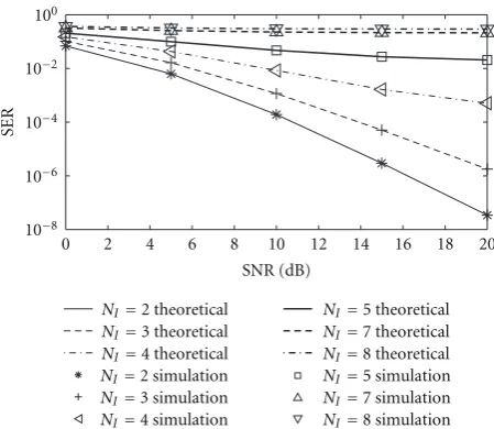
Figure2: SER versus average SNR with diﬀerent values ofNIwhen L=4,K=6, and SIR=0 dB.

We conclude that the diversity order of the whole system is aﬀected by the number of the interferersNI, the number of the relay nodesK, and the number of the relay antennasL. In Section 4, we show how these parameters aﬀect the diversity order through simulations.

4. Numerical Results

In this section, we verify our theoretical results through Monte-Carlo simulations. Simulations are carried out under the following settings: (1) the pathloss exponent is μ = 2, (2) the SNR in the simulations is defined as Ps/σ2 and

σ2 ₌ _{1, (3) it is assumed that one OFDM symbol has} Nsub = 64 subcarriers, and (4) we also assume thatLtap =

6 and the power delay profile of each channel is uniform; that is, the tap of each channel is modeled as a zero-mean Gaussian random variable with varianceσ2

x/Ltap, where

x ∈ {SRk,ImRk,RkD,ImD, m = 1,. . .,NI,k =1,. . .,K}. A pseudorandom frequency interleaver [29] is used, so after deinterleaving adjacent subcarriers become approximately uncorrelated.

For various values of NI,L, and K, average signal-to-interference ratio (SIR) per branchPs/PI and average SNR per branch Ps/σ2, we compare the simulation values with

our theoretical results, using QPSK modulation as one case of M-PSK. Meanwhile, we compare the SER performance of diﬀerent modulation such as BPSK, QPSK, and 8PSK. In Figures 2–4 and Figure 6, we assume all interferers are generated as Gaussian distribution, but inFigure 5, both the desired signal and the interference signal are assumed to be QPSK. From these figures, we can find that the theoretical results match the simulation results well.

Figure 2shows the SER performance of the considered system versus average SNR per branchPs/σ2with diﬀerent

(10)

2 3 4 5 6 8 K

NI=2 theoretical NI=4 theoretical NI=6 theoretical NI=8 theoretical

NI=2 simulation NI=4 simulation NI=6 simulation NI=8 simulation 10−6

10−5 10−4 10−3 10−2 10−1 100

SER

7

Figure3: SER versusKwith diﬀerent values ofNI whenL = 6,

SIR=0 dB, and SNR=10 dB.

2 3 4 5 6 7 8

L

NI=2 simulation NI=4 simulation NI=6 simulation NI=8 simulation 10−4

10−3 10−2 10−1

SER

NI=2 theoretical

Figure4: SER versusLwith diﬀerent values ofNIwhenK=6 and

SIR=0 dB, and SNR=10 dB.

SNR, the SER increases as the number of the interferersNI increases and (2) whenNI < L,NI <K, for example,NI = 2 or 3, the performance of the system is satisfactory, but the performance of the system is the worst whileNI> L, NI>K. We plot the SER versus the number of the relay nodesK

with SIR = 0 dB, SNR = 10 dB forL = 6 inFigure 3. In this figure, we considerNI = 2, 4, 6, 8. From this figure, it can be shown that: (1) for a given working SNR, the more relays there are, the smaller the SER is and (2) for a givenK, whenL >NI, the SER is smaller than that whenL≤NI, and the space between these two kinds of curves (e.g.,NI =2, 4 andNI=6, 8) becomes wider when the number of the relays becomes larger. That is to say, the increment of the number of the relay nodes can improve the SER performance of system with multiple interferers. Especially when the number of the relay antennas is large enough to combat the interferers at the relay node (i.e.,L >NI), the eﬀect of increasing the number

−4 −2 0 2 4 6

SIR (dB)

NI=2 simulation NI=5 simulation NI=8 simulation 10−4

10−3 10−2 10−1

SER

SNR=10 dB 100

Figure5: SER versus SIR with diﬀerent values ofNIwhenL=4, K=6, QPSK interferers.

0 2 4 6 8 10 12 14 16 18 20 10−12

10−10 10−8 10−6 10−4 10−2 100

SER

NI=2 BPSK theoretical NI=2 QPSK theoretical NI=2 8PSK theoretical NI=2 BPSK simulation NI=2 QPSK simulation NI=2 8PSK simulation

NI=5 BPSK theoretical NI=5 QPSK theoretical NI=5 8PSK theoretical NI=5 BPSK simulation NI=5 QPSK simulation NI=5 8PSK simulation SNR (dB)

NI=5

NI=2

Figure6: SER versus SNR with diﬀerent kinds of modulation when

L=4,K=6.

of the relay nodes to combat the interferers will become more eﬀective.

(11)

Combining Figures 3 and 4, we can get the fact that increasing the number of the relay nodes, and the number of both relay antennas can improve the SER performance of the system because of increasing diversity order, but the effect of the former is more evident. That is to say, the number of the relay nodes affects the diversity order of the system more greatly. From Figures3and4, we find that the diversity order can combat the interferers effectively, so if we can not utilize enough numbers of the relays and relay antennas simultaneously, it had better to utilize as many as possible relay nodes to increase the diversity order of the system for improving the SER performance.

In Figure 5, we plot the SER versus average SIR per branch Ps/PI with SNR = 10 dB, L = 4 and K = 6, using diﬀerent values ofNI, and the interference signals are generated as QPSK symbols. From this figure, it can be seen that: (1) although the interference signals are not Gaussian distributed, the simulation results are still very close to the theoretical results. That is to say, the Gaussian assumption for the interference which is necessary for obtaining the theoretical results is not critical for the accuracy of the SER expressions. A similar conclusion was drawn in [30]. In fact, it is well known that OC maximizes the SINR, irrespective of the density function governing the interference [30]; (2) it is obvious that the increase of SIR can improve the SER performance of the system. Although the SER increases with the increase ofNIfor a given SIR, the more interferers there are in the system, the faster the rate at which the SER falls with the increase in SIR is.

The SER performances of the system versus SNR with

M-PSK (M =2, 4, 8) modulation are presented inFigure 6. Among BPSK, QPSK, and 8PSK modulation modes, the SER performance of 8PSK is worst while that of BPSK is best.

5. Conclusion

In this paper, we consider an OFDM-based multiple DF relays network over frequency-selective Rayleigh fading channels and derive an unified closed-form expression of average SER for M-PSK modulation in the presence of multiple interferers. Monte-Carlo simulations are carried out to verify our theoretical results.

In the practical OFDM-based relay network, the corre-lation among the subcarrier channels is unavoidable, and the performance analysis becomes more diﬃcult. Hence, we consider it as a future work.

Appendices

A. ϕ

m

(

a

,

b

)

ϕm(a,b) is defined as follows:

ϕm(a,b)=

_∞

0

λmIk(n) exp

−λIk(n)

λIk(n) +a

×arctan ⎛ ⎝ b

λIk(n) +a

⎞ ⎠_dλ_I_k(n),

a >0, m=0, 1, 2,. . . .

(A.1)

In order to evaluateϕm(a,b), we first change the variable

of integration tov=λIk(n) +a, so

ϕm(a,b)=

∞

a

(v−a)mexp(a−v) √

v arctan

b √ v

dv. (A.2)

Using the binomial expansion of (v−a)m, (A.2) can be rewritten as

ϕm(a,b)=exp(a) m

i=0

⎛ ⎝m

i ⎞ ⎠₍_−a₎m−i

× _∞

a v

i−1/2_exp(_−v_{) arctan}_bv−1/2_dv.

(A.3)

Now, let us focus on the evaluation ofRi(a,b) which is

defined as follows:

Ri(a,b)=

_∞

a v

i−1/2_exp(_−v_{) arctan}_bv−1/2_dv. _(A.4)

Integrating by parts, we obtain the following expression from (A.4):

Ri(a,b)=ai−1/2arctan

ba−1/2_exp(_−a₎

+

i−1 2

∞

a

exp(−v)vi−3/2_arctan_bv−1/2_dv

−b 2

_∞

a exp(−v)

vi−2

1 +b2_v−1dv

=ai−1/2_arctan_ba−1/2_exp(_−a₎

+

i−1 2

Ri−1(a,b)−b

2Fi(a,b),

(A.5)

whereFi(a,b)=

1∞

a exp(−v)(vi−2/(1 +b2v−1))dv.

Now, our task is to obtain the closed-form expression of Fi(a,b). Because

Fi(a,b)=

_∞

a exp(−v)

vi−1

v+b2dv

=

i

j=2

(−1)j−2b2(j−2)

_∞

a exp(−v

)vi−j_dv

+ (−1)i−1b2(i−1)

∞

a

exp(−v) v+b2 dv.

(A.6)

With the help of [31, 8.350.2.11],1a∞exp(−v)vi−jdvin (A.6)

can be expressed as _∞

a exp(−v)v

i−j_dv₌_Γ_i₋_j_{+ 1,}_a_. _(A.7)

And with the help of [31, 3.352.2],1_a∞(exp(−v)/(v+b2₎₎_dv

in (A.6) can be expressed as ∞

a

exp(−v)

v+b2 dv= −e b2

(12)

Thus, (A.6) can be rewritten as

Fi(a,b)= i

j=2

(−1)j−2b2(j−2)Γi−j+ 1,a

−(−1)i−1b2(i−1)eb2Ei−a−b2.

(A.9)

After obtaining the closed-form expression ofFi(a,b), we

can solve the diﬀerence equation (A.5) to yield [32]

Ri(a,b)=Γ(_Γi+ 0.5)

(0.5) R0(a,b) + arctan

ba−1/2_exp(_−a₎

×

i

p=1

Γ(i+ 0.5) Γp+ 0.5a

p−1/2

−b 2

i

p=1

Γ(i+ 0.5)

Γp+ 0.5Fp(a,b),

(A.10)

whereΓ(·) denotes the gamma function, andR0(a,b), which is the value of (A.4) wheni=0, can be calculated beforehand and used as the known constant value.

Substituting (A.9) and (A.10) into (A.3), we can obtain the closed-form expression forϕm(a,b)

ϕm(a,b)=exp(a) m

i=0

⎛ ⎜ ⎝ m

i ⎞ ⎟

⎠(−a)m−iRi(a,b). (A.11)

B. P

k,n

(

e

)

Let

IL−NI

(M−1)π M ;c1,c2

= 1 π

(M−1)π/M

0

⎛

PSKPSσSR2k/σ

2

⎞ ⎠

L−NI

× ⎛

⎝ sin2θ

sin2_θ₊_g

PSKPSσSR2k/

PIσI2RkλIk,l(n) +σ2

⎞ ⎠_dθ_,

(B.1)

wherec1 =gPSKPSσSR2k/σ

2_,_c

2 = gPSKPSσSR2k/(PIσ

2

IRkλIk,l(n) +

σ2_{), using the same technique as in the case of}_N

I ≥ L, we

can get the following expression:

Pk,n(e)=

1

NI NI

l=1(NI−l)!(L−l)!

× NI

l=1

∞

0 λ L−NI Ik,l (n) exp

−λIk,l(n)

×IL−NI

(M−1)π M ;c1,c2

⎡ ⎣NI−1

p=0

βpλIpk,l(n)

⎤ ⎦_dλ_I

k,l(n),

(B.2)

whereβp (p=0, 1,. . .,NI−1) are the same form as (26) with LandNIexchanged.

From [21, 5A.17] and [21, 5A.56], we know that

IL−NI

(M−1)π

M ;c1

= 1 π

(M−1)π/M

0

, sin2_θ

sin2_θ₊_c 1

-L−NI dθ

=(M−1)

M −

1 π

. c1

1 +c1

× ⎧ ⎨ ⎩

_π

2+ arctanα

×

m−1

p=0

⎛ ⎝2p

p ⎞

⎠ 1

(4(1 +c1))p

+ sin(arctanα)×

m−1

p=1 p

t=1

Ttp

(1 +c1)p

×[cos(arctanα)]2(p−t)+1 ⎫ ⎬ ⎭,

IL−NI

(M−1)π M ;c1,c2

=IL−NI

(M−1)π

M ;c1

−T2

π .

c2

1 +c2

c2

c2−c1

L−NI

+T1 π

. c1

1 +c1 L−NI−1

q=0

c2

c2−c1

L−NI−q ⎛ ⎝2q

q ⎞ ⎠

× 1

[4(1 +c1)]q

+ 2 π

. c1

1 +c1 L−NI−1

q=0 q−1

t=0

c2

c2−c1

L−NI−q

× ⎛ ⎝2q

t ⎞

⎠_× (−1)t+q [4(1 +c1)]q

sin/2q−2tT1

0

2q−2t ,

(B.3)

where Tt p = (2pp)/((2(pp−−tt))4t[2(p − t) + 1]), α =

c1/(1 +c1)cot (π/M),Tp=(1/2) arctan(Np/Dp)+(π/2)[1−

sgn(Np)((1 + sgn(Dp))/2)],Np =2

cp(1 +cp) sin 2φ,Dp =