A Robust Statistical-Based Speaker's Location Detection Algorithm in a Vehicular Environment

(1)

Volume 2007, Article ID 13601,11pages doi:10.1155/2007/13601

Research Article

A Robust Statistical-Based Speaker’s Location Detection

Algorithm in a Vehicular Environment

Jwu-Sheng Hu, Chieh-Cheng Cheng, and Wei-Han Liu

Department of Electrical and Control Engineering, National Chiao Tung University, Hsinchu 300, Taiwan

Received 1 May 2006; Revised 27 July 2006; Accepted 26 August 2006

Recommended by Aki Harma

This work presents a robust speaker’s location detection algorithm using a single linear microphone array that is capable of detect-ing multiple speech sources under the assumption that there exist nonoverlapped speech segments among sources. Namely, the overlapped speech segments are treated as uncertainty and are not used for detection. The location detection algorithm is derived from a previous work (2006), where Gaussian mixture models (GMMs) are used to model location-dependent and content and speaker-independent phase diﬀerence distributions. The proposed algorithm is proven to be robust against the complex vehicular acoustics including noise, reverberation, near-filed, far-field, line-of-sight, and non-line-of-sight conditions, and microphones’ mismatch. An adaptive system architecture is developed to adjust the Gaussian mixture (GM) location model to environmental noises. To deal with unmodeled speech sources as well as overlapped speech signals, a threshold adaptation scheme is proposed in this work. Experimental results demonstrate high detection accuracy in a noisy vehicular environment.

Copyright © 2007 Jwu-Sheng Hu et al. This is an open access article distributed under the Creative Commons Attribution License, which permits unrestricted use, distribution, and reproduction in any medium, provided the original work is properly cited.

1. INTRODUCTION

Electronic systems, such as mobile phones, global position-ing systems (GPS), CD or VCD players, air conditioners, and so forth, are becoming increasingly popular in vehicles. In-telligent hands-free interfaces, including human-computer interaction (HCI) interfaces [1–3] with speech recognition, have recently been proposed due to concerns over driving safety and convenience. Speech recognition suﬀers from en-vironmental noises, explaining why speech enhancement ap-proaches using multiple microphones [4–7] have been intro-duced to purify speech signals in noisy environments. For example, in vehicle applications, a driver may wish to exert a particular authority in manipulating the in-car electronic systems. Additionally, for speech signal purification, a better receiving beam using a microphone array can be formed to suppress the environmental noises if the speaker’s location is known.

The concept of employing a microphone array to localize sound source has been developed over 30 years [8–15]. How-ever, most methods do not yield satisfactory results in highly reverberating, scattering or noisy environments, such as the phase correlation methods shown in [16]. Consequently, Brandstein and Silverman proposed Tukey’s Biweight to the

(2)

Mi

cr

oph

o

n

e

ar

ra

y

Digitalized

data Voice activity detector

VAD=1

VAD=0

Speech stage

Speech detected

Y1(ω)

Y2(ω)

YM(ω)

Location detector .

. .

Silent stage

Nonspeech detected

N1(ω)

N2(ω)

NM(ω)

X1(ω)

X2(ω)

XM(ω)

S1(ω)S2(ω) SM(ω) +

+

+ .

. .

. . .

Prerecorded speech database

Location model training procedure

Model parameters Detection

result

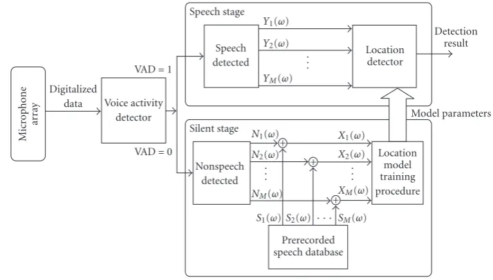
Figure1: Overall system architecture.

Our previous work [27] utilizes Gaussian mixture model (GMM) [28] to model the phase diﬀerence distributions of the desired locations as location-dependent features for speaker’s location detection. The proposed method in [27] is able to overcome the nonideal properties mentioned above and the experimental results indicate that the GMM is very suitable for modeling these distributions under both non-line-of-sight and non-line-of-sight conditions. Additionally, the proposed system architecture can adapt the Gaussian mix-ture (GM) location models to the changes in online envi-ronmental noises even under low-SNR conditions. Although the work in [27] proved to be practical in vehicular environ-ments, it still has several issues to be solved.

First, the work in [27] assumed that the speech signal is emitted from one of the previously modeled locations. In practice, we may not want to or could not model all posi-tions. In this case, an unexpected speech signal which is not emitted from one of the modeled locations, such as the radio broadcasting from the in-car audio system and the speaker’s voices from unmodeled locations, could trigger the voice ac-tivity detector (VAD) in the system architecture, resulting in an incorrect detection of the speaker location. Second, if the speech signals from various modeled locations are mixed together (i.e., the speech signals are overlapped speech seg-ments), then the received phase diﬀerence distribution be-comes an unmodeled distribution, leading to a detection er-ror. Therefore, this work proposes a threshold-based location detection approach that utilizes the training signals and the trained GM location model parameters to determine a suit-able length of testing sequence and then obtain a threshold of thea posterioriprobability for each location to resolve the two issues. Experimental results show that the speaker’s loca-tion can be accurately detected and demonstrate that sound sources from unmodeled locations and multiple modeled locations can be discovered, thus preventing the detection error.

The remainder of this work is organized as follows. Section 2discusses the system architecture and the relation-ship between the selected frequency and microphone pairs. Section 3 presents the training procedure of the proposed GM location model and the location detection method. Section 4 shows the detection performance in single and multiple speakers’ cases, and the cases of radio broadcast-ing and speech from unmodeled locations. Conclusions are made inSection 5.

2. SYSTEM ARCHITECTURE AND MICROPHONE PAIRS SELECTION

2.1. Overall system architecture

(3)

1 2 3 M

d

2d

. . .

(M 1)d

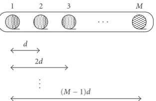
Figure2: Uniform linear microphone array geometry.

Environmental noises without speech are recorded on-line in the silent stage. Given that the environmental noises are assumed to be additive, the signals received when a speaker is talking in a noisy vehicular environment can be expressed as a linear combination of the speech sig-nal and the environmental noises. Therefore, in this stage, the system combines the online recorded environmental noise, N1(ω),. . .,NM(ω), and the pre-recorded speech sig-nals, S1(ω),. . .,SM(ω), to construct the training signals, X1(ω),. . .,XM(ω), whereMdenotes the number of micro-phones. The training signal is transmitted to the location model training procedure described inSection 3to extract the corresponding phase diﬀerences and then derive the GM location models. Since the acoustical characteristics of the environmental noises may change, the GM location model parameters are updated in this stage to ensure the detection accuracy and robustness. In the speech stage, the GM loca-tion model parameters derived from the silent stage are du-plicated into the location detector to detect the speaker’s lo-cation.

2.2. Frequency band divisions based on a uniform

linear microphone array

With the increase of the distances between microphones, the phase diﬀerences of the received signals become more sig-nificant. However, the aliasing problem occurs when this distance exceeds half of the minimum wavelength of the received signal [31]. Therefore, the distance between pairs of microphones is chosen according to the selected fre-quency band to obtain representative phase diﬀerences to en-hance the accuracy of location detection and prevent alias-ing.

Figure 2illustrates a uniform linear microphone array withMmicrophones and distanced. According to the geom-etry, the processed frequency range is divided into (M−1) bands listed in Table 1, where m denotes the mth micro-phone;brepresents the band number,νdenotes the sound velocity, and Jb is the number of microphone pairs in the band of b. The phase diﬀerences measured by the micro-phone pairs at each frequency component,ω(belonging to a specific band,b) are utilized to generate a GM location model with the dimension ofJb. An example of the frequency band selection can be found inSection 4.

3. GAUSSIAN MIXTURE LOCATION MODEL TRAINING PROCEDURE AND LOCATION DETECTION METHOD

3.1. GM location model description

If the GM location model at location l is represented by the parameter λλλ(l) = {λλλ(ω,b,l)}|M−1

b=1, then a group ofL GM location models can be represented by the parameters, {λλλ(1),. . .,λλλ(L)}. A Gaussian mixture density in the bandb at locationlcan be denoted as a weighted sum ofNGaussian component densities:

Gb

θX(ω,b,l)|λλλ(ω,b,l)

= N

i=1

ρi(ω,b,l)gi

θX(ω,b,l)

,

(1)

whereρi(ω,b,l) is theith mixture weight,gi(θX(ω,b,l)) de-notes theith Gaussian component density, andθX(ω,b,l)= [θX(ω, 1,l)· · ·θX(ω,Jb,l)]T is a Jb-dimensional training phase diﬀerence vector derived from the training signals, X1(ω),. . .,XM(ω), as shown in the following equation:

θX(ω,j,l)= phase

Xj+M−Jb(ω)

−phaseXj(ω)

with 1≤j≤Jb. (2)

The GM location model parameter in the bandbat loca-tionl,λλλ(ω,b,l), is constructed by the mean matrix, covari-ance matrices, and mixture weights vector fromNGaussian component densities

λλλ(ω,b,l)=ρ(ω,b,l),μμμ(ω,b,l),Σ(ω,b,l), (3)

whereρ(ω,b,l)=[ρ1(ω,b,l)· · ·ρN(ω,b,l)] denotes the mix-ture weights vector in the bandbat locationl.μμμ(ω,b,l) = [μ1(ω,b,l)· · ·μN(ω,b,l)] denotes the mean matrix in the bandbat locationl.Σ(ω,b,l)=[Σ1(ω,b,l)· · ·ΣN(ω,b,l)] denotes the covariance matrix in the bandbat locationl.

Theith corresponding vector and matrix of the parame-ters defined above are

μi(ω,b,l)=

μi(ω, 1,l)· · ·μi

ω,Jb,l T

,

Σi(ω,b,l)= ⎡ ⎢ ⎢ ⎢ ⎣

σi2(ω, 1,l) 0 0

0 . .. 0

0 0 σ2

i

ω,Jb,l

⎤ ⎥ ⎥ ⎥ ⎦.

(4)

Notably, the mixture weight must satisfy the constraint that

N

i=1

ρi(ω,b,l)=1. (5)

(4)

Table1: Relationship of frequency bands to the microphone pairs.

Frequency band Microphone pairs The number of microphone pairs The range of frequency band

Band 1 (b=1) (m,m+M−1) withm=1 Jb=J1=1 0< ω≤ ν

2(M−1)d

Band 2 (b=2) (m,m+M−2) with 1≤m≤2 Jb=J2=2 ν

2(M−1)d < ω≤

ν

2(M−2)d

..

. ... ... ...

BandM−1 (b=M−1) (m,m+ 1) with 1≤m≤M−1 Jb=JM−1=M−1 ν

4d < ω≤

ν

2d

3.2. GM location models training procedure and

parameters estimation

Several techniques are available for determining the param-eters of the GMM,{λλλ(1),. . .,λλλ(L)}, from the received phase diﬀerences. The most popular method is the EM algorithm [33] that estimates the parameters by using an iterative scheme to maximize the log-likelihood function shown as follows:

log₁₀pθX(ω,b,l)|λλλ(ω,b,l)

= T

t=1

log₁₀pθX(t)(ω,b,l)|λλλ(ω,b,l)

, (6)

whereθθθX(ω,b,l)= {θX(1)(ω,b,l),. . .,θX(T)(ω,b,l)}is a se-quence ofTinput phase diﬀerence vectors.

The EM algorithm can guarantee a monotonic increase in the model’s log-likelihood value and its iterative equations corresponding to frequency band selection can be arranged as follows.

Expectation step

Gb

i|θX(t)(ω,b,l),λλλ(ω,b,l)

= ρi(ω,b,l)gi

θX(t)(ω,b,l) N

i=1ρi(ω,b,l)gi

θX(t)(ω,b,l)

, (7)

whereGb(i|θX(t)(ω,b,l),λλλ(ω,b,l)) is aposteriori probabil-ity.

Maximization step

(i) Estimate the mixture weights

ρi(ω,b,l)= 1 T

T

t=1 Gb

. (8)

(ii) Estimate the mean vector

μi(ω,b,l)= T

t=1Gb

θX(t)(ω,b,l) T

t=1Gb

.

(9)

(iii) Estimate the variances

σ2 i(ω,j,l)

= T

t=1Gb

θX(t)2(ω,j,l) T

t=1Gb

−μi2(ω,j,l) with 1≤ j≤Jb,

(10)

wherei= {1,. . .,N}.

According to the work in [27], the location can be de-termined by finding the GM location model which has the maximumposterioriprobability for a given phase diﬀerence testing sequences:

l=arg max 1≤l≤L

M−1

b=1

log₁₀Gb

λλλ(ω,b,l)|θθθY(ω,b)

=arg max 1≤l≤L

M−1

b=1 log₁₀Gb

θθθY(ω,b)|λλλ(ω,b,l)

pλλλ(ω,b,l) pθθθY(ω,b)

,

(11)

where θθθY(ω,b) = {θY(1)(ω,b),. . .,θY(Q)(ω,b)} is a phase diﬀerence testing sequence derived fromY1(ω),. . .,YM(ω), andQdenotes the length of the testing sequence. However, (11) only suits for the speech signals that are emitted from one of the previously modeled locations. An unexpected speech signal which is not emitted from one of the modeled locations or a speech signal combined by the signals from various modeled locations could trigger the VAD, resulting in an incorrect detection of the speaker location. Furthermore, how to find a suitable length of the testing sequence is also an important issue.

(5)

threshold identifies the segments in which probably only one speaker in a modeled location is talking, and returns a valid location detection result.

The lengths of testing sequences and thresholds can be derived using the estimated parameters of theLGM loca-tion models. The most suitable length of testing sequences at locationl is denoted asQ(l), the threshold at locationl is denoted asζ(l), and the possible searching range of the length of the testing sequence is set to [Q−,Q+].T denotes the total length of the training phase difference sequence. θθθX,Q(ω,b,l,t)= {θX(t)(ω,b,l),. . .,θX(t+Q−1)(ω,b,l)}is a se-quence ofQtraining phase difference vectors, where 1≤t≤ T−Q+ 1. The threshold varies with different length of test-ing sequences, soQ(l) should be determined first. To obtain a representative threshold for each location, the length of test-ing sequence is decided first. A suitable length of testtest-ing se-quence should provide a robust characteristic under the GM location model, and a clear discrimination level between the locationland the other modeled or unmodeled GM loca-tions. Consequently,Q(l) andζ(l) can be obtained using the following criteria:

Q(l)=arg max Q−≤Q≤Q+

C(Q), (12)

where

C(Q)=αP−λλλ(l),θθθX(l),Q

−P+

λλλ(l),θθθX(l),Q

+β L

i=1 i=l

IP−λλλ(l),θθθX(l),Q

−P+

λλλ(i),θθθX(l),Q

+γP−λλλ(l),θθθX(l),Q

withα+β+γ=1 (13)

ζ(l)=P−

λλλ(l),θθθX(l),Q(l)

Q(l) , (14)

whereα,β,γare weights and

I(k)= ⎧ ⎨ ⎩k

ifk≥0,

−∞ ifk <0. (15)

P+(λλλ(l),θθθX(l),Q) andP−(λλλ(l),θθθX(l),Q) denote the proba-bility upper bound and lower bound when the length of the training phase diﬀerence sequence is Q. They are derived from the following equations:

P+

=max

∀t M−1

b=1

log₁₀Gb

λλλ(ω,b,l)|θθθX,Q(ω,b,l,t)

P−λλλ(l),θθθX(l),Q

=min

∀t M−1

b=1

log₁₀Gb

,

(16)

where

log₁₀Gb

=log₁₀

Gb

θθθX,Q(ω,b,l,t)|λλλ(ω,b,l)

pλλλ(ω,b,l) pθθθX,Q(ω,b,l,t)

.

(17)

The term p(λλλ(ω,b,l)) could be eliminated because p(λλλ(ω, b,l)) is independent to t and the probability p(θθθX,Q(ω,b, l,t)) is the same for allt. Therefore, (16) can be rewritten as

P+

=max

∀t M−1

b=1 Q−1

q=0 log₁₀Gb

θX(t+q)(ω,b,l)|λλλ(ω,b,l)

,

P−λλλ(l),θθθX(l),Q

=min

∀t M−1

b=1 Q−1

q=0 log₁₀Gb

θX(t+q)(ω,b,l)|λλλ(ω,b,l)

.

(18)

The first term of (13) represents the negative maximum probability variation of the trained model when the length of the training phase diﬀerence sequence isQ. As the value of this term increases, the corresponding selection ofQyields a more robust result under the trained GM location model. The second term of (13) is the sum of the probability dif-ferences of the locationlversus other locations and a larger value means the corresponding selection ofQhas a higher discrimination level between the location l and the other trained GM locations. Finally, a high discrimination level be-tween the locationland other unmodeled locations can be achieved if the third term of (13) is large.Figure 3shows the GM location model training procedure with the total loca-tion numberL.

3.3. Location detection method

The location is detected as

l=arg max 1≤l≤L

1 Q(l)

M−1

b=1

log₁₀Gb

λλλ(ω,b,l)|θθθY(ω,b,l)

=arg max 1≤l≤L

M−1

b=1

log₁₀Gb

θθθY(ω,b,l)|λλλ(ω,b,l)

pλλλ(ω,b,l)

Q(l)pθθθY(ω,b,l) (19) if ζ arg max 1≤l≤L

1 Q(l)

M−1

b=1

log₁₀Gb

≤max 1≤l≤L

1 Q(l)

M−1

b=1

log₁₀Gb

,

(6)

X1(ω)

X2(ω)

XM(ω) . . .

Phase diﬀerence extraction

Band 1 Band 2

Band (M 1)

Location model training procedure

θ (1)

X (ω,b, 1)θX(2)(ω,b, 1) M 1

b=1

θ (1)

X (ω,b, 2)θX(2)(ω,b, 2) M 1

b=1

. . .

θ (1)

X (ω,b,L)θX(2)(ω,b,L) M 1

b=1

Location models estimation Location 1

λλλ(ω,b, 1) M 1

b=1

Location 2

λλλ(ω,b, 2) M 1

b=1

. . . LocationL

λλλ(ω,b,L) M 1

b=1

Location 1

Q(1),ζ(1)

Location 2

Q(2),ζ(2)

LocationL

Q(L),ζ(L)

. . . . . .

Thresholds and the most suitable lengths of testing sequence estimation

Figure3: GM location model training procedure.

whereθθθY(ω,b,l)= {θY(1)(ω,b),. . .,θY(Q(l)) (ω,b)}is a test-ing sequence derived from Y1(ω),. . .,YM(ω). If the proba-bility densities at all locations are equally likely, then p(λλλ(ω, b,l)) could be chosen as 1/L. The probabilityp(θθθY(ω,b,l)) is the same for all location models and then the detection rule can be rewritten as

l=arg max 1≤l≤L

1 Q(l)

M−1

b=1 Q(l)

q=1

log₁₀Gb

θY(q)(ω,b)|λλλ(ω,b,l)

(21)

if

ζ

arg max 1≤l≤L

1 Q(l)

M−1

b=1 Q(l)

q=1

log₁₀Gb

≤max 1≤l≤L

1 Q(l)

M−1

b=1 Q(l)

q=1

log₁₀Gb

.

(22)

If the value of

max 1≤l≤L

M−1

b=1 Q(l)

q=1 log₁₀

Gb

Q(l) (23)

is not larger than the corresponding threshold, then the seg-ments may contain speech components that come simultane-ously from multiple modeled locations or from unmodeled locations.

4. EXPERIMENTAL RESULTS

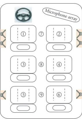
The experiment was performed in a minivan with six seats [34] (L =6).Figure 4shows the locations of the six in-car loudspeakers and the locations that are tested for the exper-iment. The first six locations correspond to modeled loca-tions, and the radio broadcasting emits from the six in-car loudspeakers, locations no. 7, 8, and 9 correspond to unmod-eled locations. A uniform linear array of six oﬀ-the-shelf, low-cost and noncalibrated microphones with 5 cm spacing

Microphone array

1 7 2

3 8 4

5 9 6

Figure4: Locations number of the seats.

is mounted in front of location no. 2. Additionally, the dis-tance between the microphone array and the mouth of the speaker who sits in location no. 2 is about 0.62 m. In this ex-periment, locations no. 1 and 2 are in the near-field condi-tion, and the signals from locations no. 3 and 5 are regarded as the far-field source according to the definition in [35]. Moreover, locations no. 4 and 6 are under the non-line-of-sight condition because the direct paths to the microphone array are sheltered by the speaker at location no. 2. The sam-pling rate is 8 kHz, and the A/D resolution is 16 bits. The processing window for calculating phase diﬀerences contains 256 zero-padded samples, and 32 milliseconds speech signals (512 samples in total). All windows are closed during the ex-periment to protect the microphones from saturation, and the cabinet temperature was set to 24◦C using the in-car air conditioner.

(7)

4 3 2 1 0 1 2 3 4 0 5 10 15 20 25 30 35 40

Phase diﬀerence (rad)

Hi

st

o

gr

am

(a) Location number 1

4 3 2 1 0 1 2 3 4

0 5 10 15 20 25 30 35 40

Hi

st

o

gr

am

(b) Location number 2

4 3 2 1 0 1 2 3 4

0 5 10 15 20 25 30 35 40

Hi

st

o

gr

am

(c) Location number 3

4 3 2 1 0 1 2 3 4

0 5 10 15 20 25 30 35 40

Hi

st

o

gr

am

(d) Location number 4

4 3 2 1 0 1 2 3 4

0 5 10 15 20 25 30 35 40

Hi

st

o

gr

am

(e) Location number 5

3 2 1 0 1 2 3 4

0 5 10 15 20 25 30 35 40

Hi

st

o

gr

am

(f) Location number 6

4 3 2 1 0 1 2 3 4

0 5 10 15 20 25 30 35 40

Hi

st

o

gr

am

(g) Location number 7

4 3 2 1 0 1 2 3 4

0 5 10 15 20 25 30 35 40

Hi

st

o

gr

am

(h) Location number 8

4 3 2 1 0 1 2 3 4

0 5 10 15 20 25 30 35 40

Hi

st

o

gr

am

(i) Location number 9

4 3 2 1 0 1 2 3 4

0 5 10 15 20 25 30 35 40

Hi

st

o

gr

am

(j) Radio broadcasting

4 3 2 1 0 1 2 3 4

0 5 10 15 20 25 30 35 40

Hi

st

o

gr

am

(k) Locations numbers 1 and 2 Figure5: Various histograms of phase diﬀerences.

which is in the third frequency band. The histogram of phase diﬀerence in an overlapped speech segment derived when two passengers at locations no. 1 and 2 speak simultane-ously is also shown inFigure 5. These phase diﬀerences are

(8)

Table2: SNR ranges at various speeds.

SNR ranges (dB)

Speed (km/h) Multiple speakers at locations

no. 1 to 6 (1–5 speakers)

Radio broadcasting

Single speaker at location no. 7

Speed=0 km/h 10.81–18.15 dB 13.10 dB 14.96 dB 13.18 dB 17.31 dB

Speed=60 km/h −0.54–6.81 dB 1.75 dB 3.81 dB 2.03 dB 5.16 dB

Speed=80 km/h −5.32–2.02 dB −3.04 dB −0.98 dB −2.76 dB 1.37 dB

Speed=100 km/h −7.28–0.07 dB −5.99 dB −2.93 dB −4.71 dB −0.58 dB

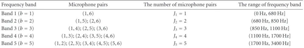
Table3: The frequency bands correspond to the microphone pairs.

Frequency band Microphone pairs The number of microphone pairs The range of frequency band

Band 1 (b=1) (1, 6) J1=1 (0 Hz, 680 Hz]

Band 2 (b=2) (1, 5); (2, 6) J2=2 (680 Hz, 850 Hz]

Band 3 (b=3) (1, 4); (2, 5); (3, 6) J3=3 (850 Hz, 1100 Hz]

Band 4 (b=4) (1, 3); (2, 4); (3, 5); (4, 6) J4=4 (1100 Hz, 1700 Hz]

Band 5 (b=5) (1, 2); (2, 3); (3, 4); (4, 5); (5, 6) J5=5 (1700 Hz, 3400 Hz]

phase difference distributions are quite different, as indicated by several research reports [36, 37]. Even locations no. 2, 4, and 6 which have the same angle to the microphone ar-ray cannot provide the similar distributions; given why these locations are distinguishable by pattern matching methods. Notably, the phase difference distribution from two simulta-neously speaking passengers at locations no. 1 and 2 is not similar to the one from location no. 1 or 2, and thus may lead to a detection error. This phenomenon indicates that a properly selected threshold for each location can avoid the detection error caused by unmodeled locations and the over-lapped speech segments.

The environmental noises are varied as the vehicle runs at various speeds of 0, 20, 40, 60, 80, and 100 km/h.Table 2lists the SNR ranges at various speeds andTable 3presents the fre-quency bands that correspond to the pairs of microphones. The voice activity detection algorithm in [29] is utilized in this experiment. The total length of the training phase diﬀ er-ence sequer-enceTis set to 300 (3-second duration). The values ofQ−,Q+,α,β, andγare set to 10, 35, 0.3, 0.4, and 0.3, re-spectively.

The mixture number of GMM model has six choices, 1, 3, 5, 7, 9, and 11. The trial number for localization detec-tion is 300 for each mixture number at each speed. For the condition of a single speaker,Figure 6plots the average cor-rect rates versus mixture numbers and indicates that a single Gaussian distribution,M =1, could not yield a satisfactory performance, and that increasing the mixture number im-proves the performance.

Fifteen possible combinations, such as locations no. 1 and 2, locations no. 1 and 3, exist with two speakers talk-ing. Three, four, and five speakers talking yield 20, 15, and

6 possible combinations, respectively.Table 4lists the aver-age error rates of these conditions with a mixture number of 11. Notably, an error is defined as a detection result that does not give the location of any of these speakers. For example, if the speech signals come from locations no. 2 and 3, then an error occurs when the detection result is neither 2 nor 3. Table 5lists the average error rates of radio broadcasting and the speech signals coming from locations no. 7, 8, and 9 with a mixture number of 11. The error in the table is defined as the detection result pointing to one of the modeled locations. The work in [27] cannot deal with multiple speakers and un-modeled speech sources because the detection result is deter-mined as the location with maximum aposteriori probabil-ity. However, the experimental results inTable 5indicate that the method proposed in this work can successfully deal with these two conditions.

5. CONCLUSION

(9)

1 3 5 7 9 11 65

70 75 80 85 90 95 100

Mixture number

Cor

re

ct

ra

te

(%

)

Location one Location two Location three

(a) Locations numbers 1 to 3

1 3 5 7 9 11

60 65 70 75 80 85 90 95 100

Mixture number

Cor

re

ct

ra

te

(%

)

Location four Location five Location six

(b) Locations numbers 4 to 6 Figure6: Average correct rates versus the mixture numbers.

Table4: Average error rates at various speeds under multiple speakers’ conditions.

Speaker number

Average error rates (%)

Speed=0 km/h Speed=20 km/h Speed=40 km/h Speed=60 km/h Speed=80 km/h Speed=100 km/h

2 0.67% 1.11% 0.44% 0.67% 1.56% 1.78%

3 0.50% 1.00% 0.67% 0.50% 1.17% 1.83%

4 0.89% 0.89% 0.66% 0.44% 1.11% 1.56%

5 0.11% 0.05% 0% 0% 0.05% 0.11%

Table5: Average error rates of unmodeled locations at various speeds.

Speed (km/h)

Average error rates (%)

Radio broadcasting Single speaker at

location no. 7

Speed=0 km/h 0.22% 0% 0.06% 0.22%

Speed=20 km/h 0.28% 0% 0.17% 0%

Speed=40 km/h 0% 0% 0% 0%

Speed=60 km/h 0.06% 0% 0% 0.33%

Speed=80 km/h 0.28% 0.33% 0.33% 0.33%

Speed=100 km/h 0.33% 0% 0.39% 0.67%

ACKNOWLEDGMENTS

This work is supported in part by the National Science Coun-cil of Taiwan under Grant no. NSC 93-2218-E-009-031 and the Ministry of Education, Taiwan, under Grant no. 91-1-FA06-4-4.

REFERENCES

[1] J. G. Ryan and R. A. Goubran, “Application of near-field op-timum microphone arrays to hands-free mobile telephony,”

IEEE Transactions on Vehicular Technology, vol. 52, no. 2, pp. 390–400, 2003.

[2] K. Pulasinghe, K. Watanabe, K. Izumi, and K. Kiguchi, “Mod-ular fuzzy-neuro controller driven by spoken language

com-mands,”IEEE Transactions on Systems, Man, and Cybernetics,

Part B, vol. 34, no. 1, pp. 293–302, 2004.

[3] W. Herbordt, T. Horiuchi, M. Fujimoto, T. Jitsuhiro, and S. Nakamura, “Noise-robust hands-free speech recognition on

PDAs using microphone array technology,” inAutumn

Meet-ing of the Acoustical Society of Japan, pp. 51–54, Sendai, Japan, September 2005.

[4] S. Gannot, D. Burshtein, and E. Weinstein, “Signal enhance-ment using beamforming and nonstationarity with

appli-cations to speech,” IEEE Transactions on Signal Processing,

(10)

[5] P. Aarabi and G. Shi, “Phase-based dual-microphone robust

speech enhancement,”IEEE Transactions on Systems, Man, and

Cybernetics, Part B, vol. 34, no. 4, pp. 1763–1773, 2004. [6] J.-S. Hu and C.-C. Cheng, “Frequency domain microphone

ar-ray calibration and beamforming for automatic speech

recog-nition,” IEICE Transactions on Fundamentals of Electronics,

Communications and Computer Sciences, vol. E88-A, no. 9, pp. 2401–2411, 2005.

[7] S. Ahn and H. Ko, “Background noise reduction via dual-channel scheme for speech recognition in vehicular

environ-ment,” IEEE Transactions on Consumer Electronics, vol. 51,

no. 1, pp. 22–27, 2005.

[8] G. C. Carter, A. H. Nuttall, and P. G. Cable, “The smoothed

coherence transform,”Proceedings of the IEEE, vol. 61, no. 10,

pp. 1497–1498, 1973.

[9] C. H. Knapp and G. C. Carter, “The generalized correlation

method for estimation of time delay,”IEEE Transactions on

Acoustics, Speech, and Signal Processing, vol. 24, pp. 320–327, 1976.

[10] G. Bienvenu, “Eigensystem properties of the sampled space

correlation matrix,” inProceedings of the IEEE International

Conference on Acoustics, Speech and Signal Processing (ICASSP

’83), vol. 8, pp. 332–335, Boston, Mass, USA, 1983.

[11] M. Wax, T.-J. Shan, and T. Kailath, “Spatio-temporal

spec-tral analysis by eigenstructure methods,”IEEE Transactions on

Acoustics, Speech, and Signal Processing, vol. 32, no. 4, pp. 817– 827, 1984.

[12] H. Wang and M. Kaveh, “Coherent signal-subspace process-ing for the detection and estimation of angles of arrival of

multiple wide-band sources,”IEEE Transactions on Acoustics,

Speech, and Signal Processing, vol. 33, no. 4, pp. 823–831, 1985. [13] J. O. Smith and J. S. Abel, “Closed-form least-squares source location estimation from range-diﬀerence measurements,”

IEEE Transactions on Acoustics, Speech, and Signal Processing, vol. 35, no. 12, pp. 1661–1669, 1987.

[14] J.-S. Hu, C.-C. Cheng, W.-H. Liu, and T. M. Su, “A speaker tracking system with distance estimation using microphone

array,” inProceedings of the IEEE/ASME International

Confer-ence on Advanced Manufacturing Technologies and Education, pp. 485–494, Chiayi, Taiwan, August 2002.

[15] J.-S. Hu, T. M. Su, C.-C. Cheng, W.-H. Liu, and T. I. Wu, “A self-calibrated speaker tracking system using both audio and

video data,” inProceedings of the IEEE Conference on Control

Applications, vol. 2, pp. 731–735, Glasgow, Scotland, Septem-ber 2002.

[16] M. Omologo and P. Svaizer, “Acoustic source location in noisy

and reverberant environment using CSP analysis,” in

Proceed-ings of the IEEE International Conference on Acoustics, Speech and Signal Processing (ICASSP ’96), pp. 901–904, Atlanta, Ga, USA, May 1996.

[17] M. S. Brandstein and H. F. Silverman, “A robust method for speech signal time-delay estimation in reverberant rooms,” in

Proceedings of the IEEE International Conference on Acoustics, Speech and Signal Processing (ICASSP ’97), vol. 1, pp. 375–378, Munich, Germany, April 1997.

[18] N. Strobel and R. Rabenstein, “Classification of time delay

es-timates for robust speaker localization,” inProceedings of the

IEEE International Conference on Acoustics, Speech and Signal Processing (ICASSP ’99), vol. 6, pp. 3081–3084, Phoenix, Ariz, USA, March 1999.

[19] S. Mavandadi and P. Aarabi, “Multichannel nonlinear phase

analysis for time-frequency data fusion,” inMultisensor,

Mul-tisource Information Fusion: Architectures, Algorithms, and Ap-plications 2003, vol. 5099 ofProceedings of SPIE, pp. 222–231, Orlando, Fla, USA, April 2003.

[20] P. Aarabi and S. Mavandadi, “Robust sound localization using

conditional time-frequency histograms,”Information Fusion,

vol. 4, no. 2, pp. 111–122, 2003.

[21] D. B. Ward and R. C. Williamson, “Particle filter beamform-ing for acoustic source localization in a reverberant

environ-ment,” inProceedings of the IEEE International Conference on

Acoustics, Speech and Signal Processing (ICASSP ’02), vol. 2, pp. 1777–1780, Orlando, Fla, USA, May 2002.

[22] I. Potamitis, H. Chen, and G. Tremoulis, “Tracking of

multi-ple moving speakers with multimulti-ple microphone arrays,”IEEE

Transactions on Speech and Audio Processing, vol. 12, no. 5, pp. 520–529, 2004.

[23] J. C. Chen, K. Yao, and R. E. Hudson, “Acoustic source

localiza-tion and beamforming: theory and practice,”EURASIP

Jour-nal on Applied SigJour-nal Processing, vol. 2003, no. 4, pp. 359–370, 2003.

[24] P.-J. Chung, J. F. B¨ohme, and A. O. Hero, “Tracking of

multi-ple moving sources using recursive EM algorithm,”EURASIP

Journal on Applied Signal Processing, vol. 2005, no. 1, pp. 50– 60, 2005.

[25] B. C. Ng and C. M. S. See, “Sensor-array calibration using a

maximum-likelihood approach,”IEEE Transactions on

Anten-nas and Propagation, vol. 44, no. 6, pp. 827–835, 1996. [26] D. B. Ward, E. A. Lehmann, and R. C. Williamson, “Particle

filtering algorithms for tracking an acoustic source in a

rever-berant environment,”IEEE Transactions on Speech and Audio

Processing, vol. 11, no. 6, pp. 826–836, 2003.

[27] J.-S. Hu, C.-C. Cheng, and W.-H. Liu, “Robust speaker’s loca-tion detecloca-tion in a vehicle environment using GMM models,”

IEEE Transactions on Systems, Man, and Cybernetics, Part B, vol. 36, no. 2, pp. 403–412, 2006.

[28] D. A. Reynolds and R. C. Rose, “Robust text-independent speaker identification using Gaussian mixture speaker

mod-els,”IEEE Transactions on Speech and Audio Processing, vol. 3,

no. 1, pp. 72–83, 1995.

[29] J. Ram´ırez, J. C. Segura, C. Ben´ıtez, A. De la Torre, and ´A. Ru-bio, “Eﬃcient voice activity detection algorithms using

long-term speech information,” Speech Communication, vol. 42,

no. 3-4, pp. 271–287, 2004.

[30] I. Potamitis, “Estimation of speech presence probability in

the field of microphone array,”IEEE Signal Processing Letters,

vol. 11, no. 12, pp. 956–959, 2004.

[31] M. Brandstein and D. Ward,Microphone Arrays: Signal

Pro-cessing Techniques and Applications, chapter 2, Springer, New York, NY, USA, 2001.

[32] D. A. Reynolds and R. C. Rose, “Robust text-independent speaker identification using Gaussian mixture speaker

mod-els,”IEEE Transactions on Speech and Audio Processing, vol. 3,

no. 1, pp. 72–83, 1995.

[33] G. Xuan, W. Zhang, and P. Chai, “EM algorithms of Gaussian

mixture model and hidden Markov model,” inProceedings of

the IEEE International Conference on Image Processing (ICIP

’01), vol. 1, pp. 145–148, Thessaloniki, Greece, October 2001.

[34] Mitsubishi Motors - Savrin (http://www.sym-motor.com.tw/

savrin-1.htm).

[35] J. G. Ryan and R. A. Goubran, “Near-field beamforming for

microphone arrays,” inProceedings of the IEEE International

Conference on Acoustics, Speech and Signal Processing (ICASSP

(11)

[36] D. D. Vries, E. M. Hulsebos, and J. Bann, “Spatial fluctuations

in measures for spaciousness,”Journal of the Acoustical Society

of America, vol. 110, no. 2, pp. 947–954, 2001.

[37] X. Pelorson, J.-P. Vian, and J.-D. Polack, “On the variability of room acoustical parameters: reproducibility and statistical

validity,”Applied Acoustics, vol. 37, no. 3, pp. 175–198, 1992.

Jwu-Sheng Huwas born in Taipei, Taiwan, in 1962. He received the B.S. degree from the Department of Mechanical Engineer-ing, National Taiwan University, Taiwan, in 1984, and the M.S. and Ph.D. degrees from the Department of Mechanical Engineering, University of California at Berkeley, in 1988 and 1990, respectively. He is currently a Pro-fessor in the Department of Electrical and Control Engineering, National Chiao Tung

University, Taiwan, His current research interests include micro-phone array signal processing, active noise control, embedded sys-tem design, and robotics.

Chieh-Cheng Cheng was born in 1978. He received the B.S. and Ph.D. degrees in electrical and control engineering from National Chiao Tung University, Taiwan, in 2000 and 2006, respectively. He is the Championship of TI DSP Solutions Design Challenge in 2000 and of the national com-petition held by Ministry of Education Ad-visor Oﬃce in 2001. His research interests include sound source localization,

micro-phone array signal processing, adaptive signal processing, pattern recognition, speech signal processing, and echo and noise cancella-tions.

Wei-Han Liuwas born in Kaohsiung, Tai-wan, in 1977. He received the B.S. and M.S. degrees in electrical and control engineering from National Chiao Tung University, Tai-wan, in 2000 and 2002, respectively. He is currently a Ph.D. candidate in Department of Electrical and Control Engineering at Na-tional Chiao Tung University, Taiwan. He is the Championship of TI DSP Solutions De-sign Challenge in 2000 and of the national