Volume 2006, Article ID 38412, Pages1–11 DOI 10.1155/ASP/2006/38412
Speech Source Separation in Convolutive Environments
Using Space-Time-Frequency Analysis
Shlomo Dubnov,1Joseph Tabrikian,2and Miki Arnon-Targan2
1CALIT 2, University of California, San Diego, CA 92093, USA
2Department of Electrical and Computer Engineering, Ben-Gurion University of the Negev, Beer-Sheva 84105, Israel
Received 10 February 2005; Revised 28 September 2005; Accepted 4 October 2005
We propose a new method for speech source separation that is based on directionally-disjoint estimation of the transfer functions between microphones and sources at different frequencies and at multiple times. The spatial transfer functions are estimated from eigenvectors of the microphones’ correlation matrix. Smoothing and association of transfer function parameters across different frequencies are performed by simultaneous extended Kalman filtering of the amplitude and phase estimates. This approach allows transfer function estimation even if the number of sources is greater than the number of microphones, and it can operate for both wideband and narrowband sources. The performance of the proposed method was studied via simulations and the results show good performance.
Copyright © 2006 Shlomo Dubnov et al. This is an open access article distributed under the Creative Commons Attribution License, which permits unrestricted use, distribution, and reproduction in any medium, provided the original work is properly cited.
1. INTRODUCTION
Many audio communication and entertainment applications deal with acoustic signals that contain combinations of sev-eral acoustic sources in a mixture that overlaps in time and frequency. In the recent years, there has been a growing in-terest in methods that are capable of separating audio signals from microphone arrays using blind source separation (BSS) techniques [1]. In contrast to most of the research works in BSS that assume multiple microphones, the audio data in most practical situations is limited to stereo recordings. Moreover, the majority of the potential applications of BSS in the audio realm consider separation of simultaneous au-dio sources in reverberant or echo environments, such as a room or inside a vehicle. These applications deal with convo-lutive mixtures [2] that often contain long impulse responses that are difficult to estimate or invert.
In this paper, we consider a simpler but still practical and largely overlooked situation of mixtures that contain a combination of source signals in weak reverberation envi-ronments, such as speech or music recorded with close mi-crophones. The main mixing effect in such a case is direct path delay and possibly a small combination of multipath delays that can be described by convolution with a relatively short impulse response. Recently, several works proposed separation of multiple signals when additional assumptions
property of the signals for purposes of detecting and sepa-rating the individual sources. Recent reported results of BSS using various single-TF detection functions show excellent performance for instantaneous mixtures.
In this paper, we propose a new method for source sepa-ration in the echoic or slightly reverberant case that is based on estimating and clustering the spatial signatures (trans-fer functions) between the microphones and the sources at different frequencies and at multiple times. The trans-fer functions for each source-microphone pair are derived from eigenvectors of correlation matrices between the micro-phone signals at each frequency, and are determined through a selection and clustering process that creates disjoint sets of eigenvector candidates for every frequency at multiple times. This requires solving the permutation problem [7], that is, association of transfer function values across different fre-quencies into a single transfer function. Smoothing and asso-ciation are achieved by simultaneous Kalman filtering of the noisy amplitude and phase estimates along different frequen-cies for each source. This differs from association methods that assume smoothness of spectra of the separated signals, rather than smoothness of the transfer functions. Even when notches in room response occur due to signal reflections, these are relatively rare compared to the inherent sparseness of the source signals, which is inherent in the W-disjoint as-sumption.
Our approach allows estimation of the transfer functions between each source and every microphone, and is capable of operating for both wideband and narrowband sources. The proposed method can be used for approximate signal sepa-ration in undercomplete cases (more than two sources in a stereo recording) using filtering or time-frequency masking [8], in a manner similar to that of the W-disjoint situation.
This paper is structured in the following manner: in the next section, we review some recent state-of-the-art algo-rithms for BSS, specifically considering the nonstationary methods of independent component analysis (ICA) and the W-disjoint approaches.Section 3presents our model and the details of the proposed algorithm. Specifically, we will de-scribe the TF analysis and representation and its associated eigenvector analysis of the correlation matrices at different frequencies and multiple times. Then, we proceed to derive a criterion for identification of the single-source TF cells and clustering the spatial transfer functions. Details of the ex-tended Kalman filter (EKF) tracking, smoothing, and across-frequency association of the transfer function amplitudes and phases conclude this section. The performance of the proposed method for source separation is demonstrated in Section 5. Finally, our conclusions are presented inSection 6.
2. BACKGROUND
The problem of multiple-acoustic-source separation using multiple microphones has been intensively investigated dur-ing the last decade, mostly based on independent compo-nent analysis (ICA) methods. These methods, largely driven by advances in machine learning research, treat the separa-tion issue broadly as a density estimasepara-tion problem. A com-mon assumption in ICA-based methods is that the sources
have a particular statistical behavior, such that the sources are random stationary statistically independent signals. Us-ing this assumption, ICA attempts to linearly recombine the measured signals so as to achieve output signals that are as independent as possible.
The acoustic mixing problem can be described by the equation
x(t)=As(t), (1)
where s(t) ∈ RM denotes the vector of M source signals,
x(t)∈RNdenotes the vector ofNmicrophone signals, andA stands for the mixing matrix with constant coefficientsAnm describing the amplitude scaling between sourcemand mi-crophonen. Naturally, this formulation describes only an in-stantaneous mixture with no delays or convolution effects. In a multipath environment, each sourcemcouples with sen-sornthrough a linear time-invariant system. Using discrete timetandτ, and assuming impulse responses not exceeding lengthL, the microphone signals are
xn(t)=
M
m=1 L
τ=1
Anm(τ)sm(t−τ). (2)
Note that the mixing is now a matrix convolution between the source signals and the microphones, whereAnm(·) rep-resents the impulse response between source nand micro-phonem. We can rewrite this equation by applying the dis-crete Fourier transform (DFT):
x(ω)=A(ω)s(ω), (3)
wheredenotes the DFT of the signal. This notation assumes that either the signals and the mixing impulse responses are of short duration (shorter than the DFT length), or that an overlap-add formulation of the convolution process is as-sumed, which allows infinite duration fors(t) andx(t), but requires a short duration of theAnm(·) responses. From now on we will consider the convolutive problem by assuming separate instantaneous mixing problemsx(ω)=A(ω)s(ω) at every frequencyω. The aim of the convolutive BSS is to find filtersWmn(t) that when applied tox(t) result in new signals
y(t) that are approximately independent. In the frequency-domain formulation we have
y(ω)=W(ω)x(ω), (4)
so thaty(t) corresponds to the original sourcess(t), up to some allowed transformation such as permutation, that is, not knowing which source sm(t) appears in which output ym(t), and amplitude scaling (relative volume).
of vectorsx =(x1,x2,. . .,xN)T, whose coordinates or com-ponents correspond to the signals at theNmicrophones, we seek to find a matrixW and vectory = (y1,y2,. . .,yM)T, whose components are “as independent as possible.” Saying so, it is assumed that there exists a multivariate process with independent componentss, which correspond to the actual independent acoustic sources, such as speakers or musical instruments, and a matrix A = W−1 that corresponds to the mixing condition (up to permutation and scaling), so that x = As. Note that here and in the following we will at times drop the frequency parameterωfrom the problem formulation.
Since the problem consists of finding an inverse matrix to the modelx=As, any solution of this problem is possible only by using some prior information ofAands. Consider-ing a pairwise independence assumption, the relevant crite-rion can be described by considering the following:
∀t,k,l,τ,i= j:Esk
i(t)slj(t+τ)
=Esk i(t)
Esm
j(t+τ)
. (5)
The parameterization of different ICA approaches can be written now as different conditions on the parameters of the independence assumption. For stationary signals, the time indices are irrelevant and higher-order statistical criteria in the form of independence conditions withk,l > 1 must be considered. For stationary colored signals, it has been shown that decorrelation of multiple timestfork = l =1 allows recovery of the sources in the case of an instantaneous mix-ture, but is insufficient for the general convolutive case. For nonstationary signals, decorrelation at multiple times,t, can be used (fork=l=1) to perform the separation.
The idea behind decorrelation at multiple timestis basi-cally an extension of decorrelation at two time instances. In the case of nonmoving sources and microphones, the same linear model is assumed to be valid at different time instances with different signal statistics, with the same orthogonal sep-arating matrixW:
Wxtj,ω
=ytj,ω
, j=1,. . .,J, (6)
where the additional indexωofWimplies that we are deal-ing with multiple separation problems for different values of ω. The same formulation can be used withoutωfor a time-domain problem, which gives a solution to the instantaneous mixture problem. Considering autocorrelation statistics at time instancest1,. . .,tJ we obtainJsets of matrix equations:
Rx,tj =W− 1Λ
y,tjW−T, j=1,. . .,J, (7)
where we assume that{Λy,tj} J
j=1are diagonal since the com-ponents of yare independent. This problem can be solved using a simultaneous diagonalization of{Rx,tj}
J
j=1, without knowledge of the true covariances of y at different times. A crucial point in implementation of this method is that it works only when the eigenvalues of the matricesRx,t are
all distinct. This case corresponds in physical reality to suf-ficiently unequal powers of signals arriving from different directions, a situation that is likely to be violated in prac-tical scenarios. Moreover, since the covariance matrices are estimated in practice from short time frames, the averaging time needs to correspond to the stationarity time. An addi-tional difficulty occurs specifically for the TF representation: independence between two signals in a certain band around ωcorresponds to independence between narrowband pro-cesses, which can be revealed at time scales that are signifi-cantly longer than the window size or the effective impulse response of the bandpass filter used for TF analysis. This in-herently limits the possibility of averaging (taking multiple frames or snapshots of the signal in one time segment) with-out exceeding the stationarity interval of the signal. In the following we will show how our method solves the eigenvalue indeterminacy problem by choosing those time segments where only one significant eigenvalue occurs. Our “segmen-tal” approach actually reduces the generalized (or multiple) eigenvalue problem into a set of disjoint eigenvalue problems that are solved separately for each source. The details of our algorithm will be described in the next section. In the fol-lowing, we will consider the “directionally-disjoint” sources case in which the local covariance matricesRx,tj have a single large eigenvalue at sufficiently many time instancestj. The precise definition and the amount of times that are sufficient for separation will be discussed later.
3. PROPOSED SOURCE SEPARATION METHOD
Consider anN-channel sensor signal x(t) that arises from M unknown scalar source signalssm(t), corrupted by zero-mean, white Gaussian additive noise. In a convolutive en-vironment, the signals are received by the array after delays and reflections. We consider the case where each one of the sources has a different spatial transfer function. Therefore, the signal at thenth microphone is given by
xn(t)=
M
m=1 L
l=1
anmlsm(t−τnml) +vn(t), n=1,. . .,N,
(8)
in whichτnmlandanmlare the delay and gain of thelth path between source signal mand microphonen, andvn(t) de-notes the zero-mean white Gaussian noise. The STFT of (8) gives
Xn(t,ω)=
M
m=1
Anm(ω)Sm(t,ω) +Vn(t,ω), n=1,. . .,N,
(9)
whereSm(t,ω) andVn(t,ω) are the STFT ofsm(t) andvn(t), respectively, and the transfer function between themth signal to thenth sensor is defined as
Anm(ω)=
L
l=1
In matrix notation, the model (9) can be written in the form
X(t,ω)=A(ω)S(t,ω) +V(t,ω). (11)
Our goal here is to estimate the spatial transfer function matrix,A(ω), and the signal vector,s(t), from the measure-ment vectorx(t). For estimation of the signal vector, we will assume that the number of sources,M, is not greater than the number of sensors,N. This assumption is not required for estimation of the spatial transfer function matrix,A(ω).
The proposed approach seeks time-frequency cells in which only one source is present. At these cells, it is pos-sible to estimate the unstructured spatial transfer function matrix for the present source. Therefore, we will first iden-tify the single-source TF cells and calculate the spatial trans-fer functions for the sources present in those cells. In the second stage, the spatial transfer functions are clustered using a Gaussian mixture model (GMM). The frequency-permutation problem is solved by considering the spatial transfer functions as a frequency-domain Markov model and applying an EKF to track it. Finally, the sources are separated by inverse filtering of the measurements using the estimated transfer function matrices.
The autocorrelation matrix at a given time-frequency cell is given by
Rx(t,ω)=EX(t,ω)XH(t,ω)
=A(ω)Rs(t,ω)AH(ω) +Rv(t,ω), (12)
whereRx,Rs, andRvare the time-frequency spectra of the measurements, source signals, and sensor noises, respec-tively. We assume that the noise is stationary, and there-fore its covariance matrix is independent of timet, that is,
Rv(t,ω)=Rv(ω). Furthermore, the noise spectrum is usually known, so (12) can be spatially prewhitened by left multiply-ing (11) byR−1/2
v (ω). Thus, we can assumeRv(ω)=σv2IN for allωwhereINis the identity matrix of sizeN.
3.1. Identification of single-source TF cells
Each time-frequency window is tested in order to identify the time-frequency windows in which a single signal is present. In these cells, the unstructured spatial transfer function can be easily estimated. Consider a time segment consisting of T time cells in which the signals are stationary. Then, (12) becomes time-independent:
Rx(ω)=A(ω)Rs(ω)AH(ω) +σ2
vIN. (13)
If only themth source is present, (13) becomes
Rxm(ω)=am(ω)aHm(ω)σs2m(ω) +σ 2
vIN, (14)
where am(ω) is the mth column of the matrix A(ω) and
σ2
sm(ω) denotes themth signal power spectrum. In this case, the rank of the (noiseless) signal covariance matrix is 1 and
am(ω) is proportional to the eigenvector of the
autocorre-lation matrixRxm(ω) associated with the maximum eigen-value:λ1,m(ω)=σs2m(ω)am(ω)
2+σ2
v. This property allows us to derive a test for identification of the single-source seg-ments and estimate the corresponding spatial transfer func-tionam(ω). We will denote the eigenvector corresponding to the maximum eigenvalue of the matrixRx(ω) byu(ω), disre-garding the source indexm.
The three hypotheses for each time-frequency cell in a stationary segment, which indicate the number of active sources in this segment, are
H0:X(t,ω)∼Nc
0,σ2 vIN
,
H1:X(t,ω)∼Nc
0,u(ω)uH(ω)σ2
s(ω) +σv2IN
,
H2:X(t,ω)∼Nc
0,Rx(ω),
(15)
where H0, H1, H2 indicate noise-only, single-source, and multiple-source hypotheses, respectively, withX ∼Nc(·,·) denoting the complex Gaussian distribution. Under hypoth-esis H0, the model parameters are known. Under hypoth-esis H1, the vector u(ω) is the normalized spatial transfer function of the present source in the segment (i.e., one of the columns of the matrixA(ω)) andσ2
s(ω) represents the corresponding signal power spectrum. We assume thatu(ω) andσ2
s(ω) are unknown. In hypothesisH2, it is assumed that the data model is complex Gaussian-distributed and spatially colored with unknown covariance matrixRx(ω), which rep-resents the contribution of several mixed sources. Usually, the Gaussian distribution assumption for hypothesesH1and H2does not hold, and in fact leads to suboptimal solutions. However, this assumption enables obtaining a simple and meaningful result for source separation.
In order to identify the case of a single source, two tests are performed. In the first, the hypotheses H0 andH1 are tested, while in the second, hypothesesH1andH2are tested. A time-frequency cell is considered as a single-source cell if in both tests it is decided that a single source is present. These tests are carried out between hypotheses with unknown pa-rameters, and therefore the generalized likelihood ratio test (GLRT) is employed, that is,
H1
GLRT1=max
u,σ2
s
logfX|H1;u,σs2−logfX|H0≷γ1,
H0
H2
GLRT2=max
Rx
logfX|H2;Rx−max
u,σ2
s
logfX|H1;u,σs2≷γ2,
H1
(16)
where fX|H0, fX|H1;u,σs2, and fX|H2;Rx denote the probability density functions (pdf ’s) of each time-frequency segment under the three hypotheses.
X(t,ω)∼Nc[0,Rx(ω)]. The model ofRx(ω) differs between the three hypotheses. The log-likelihood of the dataX(ω) un-der the joint model is
logfX|Rx= −Tlog πRx(ω) − T
t=1
XH(t,ω)Rx−1(ω)X(t,ω)
= −Tlog πRx(ω) + trRx(ω)R−1
x (ω)
,
(17)
where Rx (ω) is the sample covariance matrix Rx (ω) 1/TTt=1X(t,ω)XH(t,ω). For simplicity of notation, we will drop the dependence on frequencyω.
Under hypothesisH0,Rx = σ2
vI, and therefore the log-likelihood from (17) becomes
logfX|H0= −T
Nlogπσ2
v
+ 1
σ2
v
trRx. (18)
Under hypothesisH1,Rx=σ2
suuH+σv2IN, for which the following equations are satisfied:
R−1
x =
1
σ2
v
IN− SNR 1 + SNRuu
H
, Rx =σ2N
v (1 + SNR),
(19)
where SNRσ2
s/σv2. Substitution of (19) into (17) yields
logfX|H1,u,σs2= −T
logπσ2 v
N
(1 + SNR)
+ 1
σ2
v tr
Rx
IN− SNR 1 + SNRuu
H
= −T
Nlogπσv2
+ 1
σ2
v
trRx+ log(1 + SNR)
− SNR
σ2
v(1 + SNR)
uHRxu
.
(20)
Maximization of (20) with respect to σ2
s can be replaced by maximization with respect to SNR. This operation can
be performed by calculating the derivative of (20) with re-spect to SNR and equating it to zero, resulting inSNR( u)= uHRxu /σ2
v−1 orσs2(u)=uHRxu −σv2. Thus,
max σ2
s
logfX|H1,u,σ2s
= −T
Nlogπσv2
+ 1
σ2
v
trRx+ 1 + logη−η
,
(21)
whereη uHRxu /σ2
v. We seek to maximize (21) with re-spect tou, whereuis constrained to unity norm. Since (21) is monotonically increasing withη, forη > 1, then the log-likelihood is maximized when η is maximized. Let λ1 ≥
· · · ≥λNdenote the eigenvalues ofRx . Then, maxuuHRxu = λ1, and
max
u,σ2
s
logfX|H1,u,σs2= −T
Nlogπσ2
v
+ 1 + 1
σ2
v trRx
+ logλ1
σ2
v
−λ1
σ2
v
= −T
Nlogπσv2
+ 1 +
N
i=2
λi
σ2
v
+ logλ1
σ2
v
.
(22)
Under hypothesisH2, the matrixRxis unstructured and
assumed to be unknown. Equation (17) is maximized for
Rx=Rx[9]. The resulting log-likelihood under this
hypoth-esis is
max
Rx
logfX|H2,Rx= −T
log πRx +N
= −T
Nlogπ+
N
i=1
logλi+N
. (23)
Now, the two GLRTs for decision between (H0,H1) and (H1,H2) can be derived by subtracting the corresponding log-likelihood functions:
H1
GLRT1=max
u,σ2
s
logfX|H1;u,σs2−logfX|H0=T
λ1
σ2
v
−logλ1
σ2
v
−1
≷γ1,
H0
H2
GLRT2=max
Rx
logfX|H2;Rx−max
u,σ2
s
logfX|H1;u,σs2=T N
i=2
λi
σ2
v
−log λi
σ2
v
−N+ 1
≷γ2.
H1
Finally, after dropping the constants, and modifying the thresholds accordingly, the two tests can be stated as
H1
T1=
λ1
σ2
v
−logλ1
σ2
v
≷γ1,
H0
H2
T2=
N
i=2
λi
σ2
v
−log λi
σ2
v
≷γ2.
H1
(25)
The thresholdsγ1 andγ2 in the two tests should be set according to the following considerations. Large values for γ1 and small values forγ2will lead to missed detections of single-source TF cells, and therefore lead to a lack of data for calculation of the spatial transfer function. On the other hand, small values forγ1 or large values forγ2 will lead to false detections of single-source TF cells, which can cause er-roneous estimation of the spatial transfer function. Gener-ally, larger amounts of data will enable us to increaseγ1and decreaseγ2.
In the case of stereo signals (N =2), both tests could be expressed fori=1, 2 andλ2≥λ1≥σv2as
Hi
Ti=
λi
σ2
v
−log λi
σ2
v
≷γi.
Hi−1
(26)
3.2. Spatial transfer function estimation
In the TF cells that are identified to be single-source cells, the ML estimator for the normalized spatial transfer function of the present source at the given frequencyωis given by the eigenvector associated with the maximum eigenvalue of the autocorrelation matrixRxm. It is important to note that a sin-gle amplitude-delay pair is sufficient to describe the spatial transform for a sufficiently narrow frequency band represen-tation and assuming a linear spatial system. We can rewrite the model (11) for the case of two sources and two micro-phones as
X1(ω)
X2(ω)
=
1 1
a1e−jωδ1 a2e−jωδ2
S1(ω)
S2(ω)
(27)
in which case, the mixing matrix column, corresponding to one of the sources, say sourcem, can be directly estimated from the eigenvector,am(ω), associated with the maximum eigenvalue of the autocorrelation matrixRxmunder hypoth-esisT1, that is, a single-sourcemis present in this TF region. Thus,
ame−jωδm=am,2(ω)
am,1(ω), (28)
wheream,idenotes theith component ofam, or more specif-ically
am=
aam,2(m,1(ωω)) ,
δm=
1 ω
logam,2(ω)
am,1(ω)
,
(29)
where denotes taking the imaginary part.
Having different amplitude and delay values for each source at every frequency, we need to associate the different amplitude and delay values across frequency to their corre-sponding source. If we assume that the amplitude and de-lay are constant over different frequencies, occurring in the case of a direct path effect only, the association can be per-formed by clustering the amplitude and phase values around their mean value. In the case of multipath, the amplitude and delay values may differ across frequencies. Using smooth-ness considerations, one could try to associate the parame-ters across different frequencies by assuming proximity of pa-rameter values across frequency bins for the same source. It should be also noted that smoothness of delay values requires unwrapping of the complex logarithm before dividing byω. This is limited by spatial aliasing for high frequencies, that is, if the spacingdbetween the sensors is too large, the delayd/c wherecis the speed of sound, might be larger than the max-imum permissible delay 2π/ωs, withωs denoting the sam-pling frequency. In other words, it might not be possible to uniquely solve the permutation problem if the delay between two microphones is more than one sample. Moreover, sepa-rate clustering or associating amplitude and delay parameters also looses information about the relations between the real and imaginary components of the spatial transfer function vector. In the following section, we will describe an optimal tracking and frequency association based on Kalman mod-eling, which addresses these problems assuming smoothness of the amplitude and phase of the spatial transfer function across frequency.
4. TRACKING AND FREQUENCY ASSOCIATION ALGORITHM
parameters across frequency is performed by operating sep-arate EKFs on the cluster means, one for each source.
4.1. Gaussian mixture model and extended
Kalman filter
The GMM assumes that the observationszare distributed according to the following density function
pz(z)=
M
m=1
πmN
z|Θm
, (30)
whereπmare the weights of the Gaussian distributionN(· |
Θm), andΘm= {μm,Σm}are its mean and covariance matrix parameters, respectively. In our case, the observations,z, are estimates of the real and imaginary parts of the transfer func-tion over frequency (see previous secfunc-tion). The parameters of the GMM are obtained using an expectation-maximization (EM) procedure. The estimated mean and covariance matrix at each frequency are used for tracking the spatial transfer function.
An EKF is used for tracking and association of the trans-fer functions, whose mean and variance are estimated by the EM algorithm. The idea here is that the spatial transfer func-tion between each source and microphone is smooth over frequency. Notches that occur in the transfer function due to signal reflections will be smoothed by the EKF, causing errors in the estimation (29), which color the signal but do not in-terfere with the association process since one of the sources in this case has small or zero amplitude. Therefore, the spa-tial transfer functions are modeled as first-order Markov se-quences. It is natural to use the magnitude and phase of each spatial transfer function for the state vector, because in sim-ple scenarios with no multipath, the absolute value of the transfer function is constant over frequency, while its phase linearly varies with frequency. Thus, the state vector of each EKF includes the magnitude (ρ), phase (α), and phase rate ( ˙α) of the transfer function. The presence of multipath causes deviation from this model, which can be represented by a noise model. Thus, the state vector dynamics across neigh-boring frequencies (frequency smoothness constraint) are modeled as
φk= ⎛ ⎜ ⎝αρkk
˙
αk
⎞ ⎟ ⎠=
⎛ ⎜ ⎝
1 0 0 0 1 1 0 0 1 ⎞ ⎟ ⎠ ⎛ ⎜ ⎝ρk−
1
αk−1
˙
αk−1
⎞ ⎟ ⎠+nφk,
μk=
am
ωk
am
ωk
=
ρkcosαk
ρksinαk
+nμk,
(31)
in which the noise covariance ofnμkis taken from the above-mentioned clustering algorithm, and the model noise covari-ance ofnφkis set according to the expected dynamics of the spatial transfer function.
For tracking theM transfer functions,M independent EKFs are implemented in parallel. At each frequency step, the data is associated with the EKFs according to the criterion of minimum-norm distance between the clustering estimates and theMKalman predictions.
4.2. The separation algorithm
The various steps of the algorithm can be summarized as fol-lows.
(i) Given a two-channel recording, perform a separate STFT analysis for every channel, resulting in the sig-nal model (11).
(ii) Perform an eigenvalue analysis of the cross-channel correlation matrix at each frequency, as described in Section 3, where (12) and (26) determine the transfer function.
(iii) At each frequency, determine the cluster centers of the set of amplitude ratio measurements using the GMM. (iv) Perform EKF tracking of the cluster means across fre-quency for each source to obtain an estimate of the mixing matrix as a function of frequency.
(v) If the mixing matrix is invertible, recover the signals by multiplying the STFT channels at each frequency by the inverse of the estimated mixing matrix. In case of more microphones than sources, the pseudoinverse of the mixing matrix should be used. In case of more sources than microphones, source separation can be approximately performed using time-frequency mask-ing method of [8].
(vi) Perform an inverse STFT using the associated frequen-cies for each of the sources.
Since the mixing matrix can be determined only up to a scaling factor, we assume a unit relative magnitude for one of the sources and use the amplitude ratios to determine the mixing parameters of the remaining source. This problem of scale invariance may cause a “coloration” of the recovered signal (over frequency) and is one of the possible sources of error, being common to most convolutional source separa-tion methods. Another typical problem is that the narrow-band processing corresponds to circular convolution rather than the desired linear convolution. This effectively restricts the length of the impulse response between the microphones to be less than half of the analysis window length, or in fre-quency it restricts the spectral smoothness to that of the DFT length. Since speech sources are sparse in frequency (at least for the voiced segments), it is assumed that spectral peaks of speech harmonics would not be seriously influenced by spec-tral detail smaller than one FFT bin.
5. EXPERIMENTAL RESULTS
Separation experiments were carried out for simulated mix-ing conditions. We tested the proposed algorithm under dif-ferent conditions, such as relative amplitudes of the sources, angles and amplitudes of the multipath reflections, and dif-ferent types of sound sources.
3500 3000 2500 2000 1500 1000 500 0
Frequency (Hz) 0
0.2 0.4 0.6 0.8 1 1.2 1.4
a2 /a1
Measured values
Smoothed transfer function values (a)
3500 3000 2500 2000 1500 1000 500 0
Frequency (Hz) 1
0.5 0 0.5 1 1.5 2 2.5 3
∠
a2 /a1
Measured values
Smoothed transfer function values (b)
Figure1: Amplitude and phase of two female speaker sources with nearly equal amplitude mixing conditions.
is possible due to the different phase behavior of the sig-nals, which is properly detected using the EKF tracking. The EKF parameters were set as follows. The system noise covariance matrix was set according to standard deviation (STD) of 0.1/sample in the transfer function amplitude and 0.1 rad/sample for phase. The measurement covariance ma-trices were set based on the results of the EM algorithm for GMM parameters estimation. The measurement STDs are in fact the widths of the Gaussians. The EKF parameters were also fixed in the following examples.
InFigure 2the SNR improvement for different relative positions of the sources with different relative amplitudes is presented. The SNR improvement was calculated according to the method described in [10]. The separation quality of themth source is evaluated by the ratio of the maximal en-ergy output signal and sum of energies of the remaining out-put signals when only sourcemis present at the input. One of the sources was fixed at 0◦while the other source was shifted from−40◦to 40◦. The amplitude ratio of the sources at the microphones varied from 0.8 to equal amplitude ratios. The multipath reflections occurred at constant angles of 60◦and
−40◦ with relative amplitudes of a few percent of the orig-inal. For equal amplitudes, we achieve up to 10 dB of im-provement when the sources are 40◦ apart. The angle sensi-tivity disappears when sufficient amplitude difference exists
40 30 20 10 0 10 20 30 40
DOA of source 2 (deg) 0
5 10 15 20 25 30
Improvement for source 1
SNR
impr
o
ve
ment
(dB)
Amp. ratio=0.8 Amp. ratio=0.9
Amp. ratio=0.95 Amp. ratio=1 (a)
40 30 20 10 0 10 20 30 40
DOA of source 2 (deg) 5
0 5 10 15 20 25
Improvement for source 2
SNR
impr
o
ve
ment
(dB)
Amp. ratio=0.8 Amp. ratio=0.9
Amp. ratio=0.95 Amp. ratio=1 (b)
Figure2: Improvement in SNR as a function of source angle for different relative amplitudes under weak multipath conditions.
between the sources. For an amplitude ratio of 0.8 (i.e., each microphone receives its main source at amplitude 1 and the interfering source at amplitude 0.8), we achieved 20–30 dB improvement. One should note that the above results con-tain weak multipath components. Even better improvement (50 dB or more) can be achieved for cases when no multipath is present.
The performance of the proposed method was tested also under strong multipath conditions. In this test, the two microphones measured signals from two sources. Each source signal arrives at the microphones through six diff er-ent paths. The paths of the first source are from 0◦, −5◦,
−10◦, −20◦, −30◦,−40◦, with strengths 0, −6, −7.5, −9,
−11, and−13.5 dB. The paths of the second source are from 60◦, 50◦, 40◦, 30◦, 20◦, with strengths−7.5,−9,−11,−13.5, and −17 dB, where the main path was at 0 dB with vary-ing direction. The relative amplitude of the received paths at the microphones was randomly chosen between 0.67–0.86. Figure 3shows the SNR improvement for both sources as a function of the main path direction for different relative am-plitudes.
40 30 20 10 0 10 20 30 40
DOA of source 2 (deg) 0
5 10 15 20
Improvement for source 1
SNR
impr
o
ve
ment
(dB)
Amp. ratio=0.8 Amp. ratio=0.9
Amp. ratio=0.95 Amp. ratio=1 (a)
40 30 20 10 0 10 20 30 40
DOA of source 2 (deg) 0
5 10 15 20
Improvement for source 2
SNR
impr
o
ve
ment
(dB)
Amp. ratio=0.8 Amp. ratio=0.9
Amp. ratio=0.95 Amp. ratio=1 (b)
Figure3: Improvement in SNR under strong multipath conditions as a function of source angle for different relative amplitudes.
direction. The microphones were positioned within a linear, equally spaced (LES) array with 4.5 cm intersensor spacing. The performance in this case is slightly lower than the case of two microphones versus two sources, mainly because there are fewer TF cells in which a single source is present. Ob-viously, longer data can significantly improve the results in cases of multiple sources and multiple microphones.
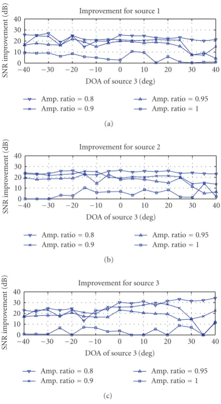
As mentioned above, the proposed method is able to esti-mate the spatial transfer function in the case of more sources than sensors.Figure 5shows the magnitude and phase of the true and estimated channel transfer functions of the three sources where only two microphones were used. The sources were located at−40◦,−10◦, and 30◦with relative amplitudes of the different sources of 4, 2, and 0.5 between the micro-phones.
Figure 6shows the amplitude of the spatial transfer func-tion obtained by the inverse mixing matrix over frequency for the case of two sources located at 0◦ and 60◦, without multipath. One can observe that the spatial pattern gen-erated by the inverse of the estimated mixing matrix in-troduces a null in the direction of the interfering source. Figure 6(a)shows the null generated around 60◦ for recov-ering the source at 0◦, whileFigure 6(b)shows the null gen-erated around 0◦for recovering the source at 60◦.
40 30 20 10 0 10 20 30 40
DOA of source 3 (deg) 0
10 20 30 40
Improvement for source 1
SNR
impr
o
ve
ment
(dB)
Amp. ratio=0.8 Amp. ratio=0.9
Amp. ratio=0.95 Amp. ratio=1 (a)
40 30 20 10 0 10 20 30 40
DOA of source 3 (deg) 0
10 20 30 40
Improvement for source 2
SNR
impr
o
ve
ment
(dB)
Amp. ratio=0.8 Amp. ratio=0.9
Amp. ratio=0.95 Amp. ratio=1 (b)
40 30 20 10 0 10 20 30 40
DOA of source 3 (deg) 0
10 20 30 40
Improvement for source 3
SNR
impr
o
ve
ment
(dB)
Amp. ratio=0.8 Amp. ratio=0.9
Amp. ratio=0.95 Amp. ratio=1 (c)
Figure4: Improvement in SNR for the case of three microphones and three sources as a function of the third source angle for different relative amplitudes.
The proposed method for estimating the spatial transfer functions using the correlation matrix of the TF representa-tion can be compared to the method for estimarepresenta-tion of mixing and delay parameters from the STFT, as reported in [3,8]. The basic assumption of that approach is the orthogonality of the “W-disjoint,” which requires that part of TF the cells in the TF representation of the sources do not overlap. The derivation of the relative amplitude and delay parameters as-sociated with sourcembeing active at (t,ω) is done using
am,δm
= X2(t,ω)
X1(t,ω)
,1
ω∠
X2(t,ω)
X1(t,ω)
. (32)
4000 3500 3000 2500 2000 1500 1000 500 0
Frequency (Hz) 0
1 2 3 4 5
The measured versus smoothed spatial transfer functions
a2 /a1
Estimated for source 1 Estimated for source 2 Estimated for source 3
Original for source 1 Original for source 2 Original for source 3 (a)
4000 3500 3000 2500 2000 1500 1000 500 0
Frequency (Hz) 1.5
1 0.5 0 0.5 1 1.5 2
∠
a2 /a1
Estimated for source 1 Estimated for source 2 Estimated for source 3
Original for source 1 Original for source 2 Original for source 3 (b)
Figure5: Channel transfer function estimation for three sources using two microphones.
and phase of the spatial transfer function for a single-source TF cell containing additive white noise. A central step in the W-disjoint approach is the clustering of the parameters in amplitude and delay space so as to identify separate sources in the mixtures. Usually this clustering step is performed un-der the assumption of constant amplitude and delay over fre-quency and is possible for speech signals when the sources are distinctly localized both in amplitude and delay. It should be noted that these methods can not handle multipath, that is, when more than one peak in the amplitude and delay space corresponds to a single source.Figure 7shows the distribu-tion of the ratio of spatial transfer funcdistribu-tion valuesa2/a1in the complex plane for two real sources over different fre-quencies at TF points that have been detected as single-TFs. It can be seen from the figure that these values have signifi-cant overlap in amplitude and phase. It is evident that simple clustering can not separate these sources and more sophisti-cated methods are required.
6. CONCLUSIONS
In this paper, we presented a new method for speech source separation based on directionally-disjoint estimation of the
80 60 40 20 0 20 40 60 80
DOA (deg) 0
5 10 15 20 25 30 35 10
2
Fre
q
u
en
cy
(H
z)
dB
60 40 20 0 20
(a)
80 60 40 20 0 20 40 60 80
DOA (deg) 0
5 10 15 20 25 30 35 10
2
F
requency
(Hz)
dB
60 40 20 0 20
(b)
Figure6: Spatial pattern obtained by the inverse of the mixing ma-trix for each frequency in the case of two sources at 0◦and 60◦.
1.5 1
0.5 0
0.5 1 1.5
Real (a2/a1) 2
1.5 1 0.5 0 0.5 1 1.5
Im
ag
e
(
a2 /a1
)
Figure7: Distribution of the ratio of spatial transfer function values
a2/a1in the complex plane for two real sources (indicated by circles
and asterisks) over different frequencies at TF points that have been detected as single-TFs.
spatial correlation matrix at single-TF instances. The advan-tage of our approach is that it allows transfer function esti-mation even in difficult conditions where the amplitudes of the mixed signals are approximately equal, and it can operate for both wideband and narrowband sources. The current work successfully extends common BSS methods that use a single-TF detection criterion to the convolutive case. The pa-per formulates single-TF detection and transfer function pa- per-mutation problems in a principled and optimal manner.
ACKNOWLEDGMENT
This work was partially supported by the Israeli Science Foundation (ISF).
REFERENCES
[1] K. Torkkola, “Blind separation for audio signals—are we there yet?” in Proceedings of 1st International Workshop on Independent Component Analysis and Blind Signal Separation (ICA ’99), pp. 239–244, Aussois, France, January 1999. [2] L. Parra and C. Spence, “Convolutive blind separation of
non-stationary sources,”IEEE Transactions on Speech and Audio Processing, vol. 8, no. 3, pp. 320–327, 2000.
[3] A. Jourjine, S. Rickard, and O. Yilmaz, “Blind separation of disjoint orthogonal signals: demixing N sources from 2 mixtures,” inProceedings of IEEE International Conference on Acoustics, Speech, and Signal Processing (ICASSP ’00), vol. 5, pp. 2985–2988, Istanbul, Turkey, June 2000.
[4] N. Roman, D. L. Wang, and G. J. Brown, “Speech segregation based on sound localization,”The Journal of the Acoustical So-ciety of America, vol. 114, no. 4, pp. 2236–2252, 2003. [5] C. Fevotte and C. Doncarli, “Two contributions to blind
source separation using time-frequency distributions,”IEEE Signal Processing Letters, vol. 11, no. 3, pp. 386–389, 2004. [6] Y. Deville, “Temporal and time-frequency correlation-based
blind source separation methods,” in Proceedings of 4th In-ternational Workshop on Independent Component Analysis and Blind Signal Separation (ICA ’03), pp. 1059–1064, Nara, Japan, April 2003.
[7] M. Z. Ikram and D. R. Morgan, “Permutation inconsistency in blind speech separation: investigation and solutions,”IEEE Transactions on Speech and Audio Processing, vol. 13, no. 1, pp. 1–13, 2005.
[8] O. Yilmaz and S. Rickard, “Blind separation of speech mix-tures via time-frequency masking,”IEEE Transactions on Sig-nal Processing, vol. 52, no. 7, pp. 1830–1847, 2004.
[9] A. Steinhardt, “Adaptive multisensor detection and estima-tion,” inAdaptive Radar Detection and Estimation, S. Haykin and A. Steinhardt, Eds., pp. 91–160, John Wiley & Sons, New York, NY, USA, 1992.
[10] D. W. E. Schobben, K. Torkkola, and P. Smaragdis, “Evalu-ation of blind signal separ“Evalu-ation methods,” inProceedings of 1st International Workshop on Independent Component Analy-sis and Blind Signal Separation (ICA ’99), Aussois, France, Jan-uary 1999.
Shlomo Dubnov received the Ph.D. de-gree in computer science from Hebrew Uni-versity of Jerusalem, Jerusalem, Israel. He holds also a B.A. degree in music composi-tion from the Rubin Academy of Mu-sic and Dance, Jerusalem. From 1996 to 1998, he worked as Invited Researcher at IRCAM, Centre Pompidou, Paris. During 1998–2003, he was a Senior Lecturer in the Department of Communication
Sys-tems Engineering at Ben-Gurion University of the Negev, Beer-Sheva, Israel. He is now an Associate Professor in the Department of Music and a Researcher at New Media Arts, CALIT2, University of California, San Diego.
Joseph Tabrikian received the B.S., M.S., and Ph.D. degrees in electrical engineering from the Tel-Aviv University, Tel-Aviv, Is-rael, in 1986, 1992, and 1997, respectively. During 1996–1998, he was with the De-partment of Electrical and Computer Engi-neering, Duke University, Durham, NC, as an Assistant Research Professor. He is now a Faculty Member in the Department of Electrical and Computer Engineering,
Ben-Gurion University of the Negev, Beer-Sheva, Israel. His research in-terests include statistical signal processing, source detection and lo-calization, and speech and audio processing. He served as an Asso-ciate Editor of the IEEE Transactions on Signal Processing during 2001–2004.