Analysis of Spaceborne Tandem Configurations for Complementing COSMO with SAR Interferometry

Analysis of Spaceborne Tandem Configurations for

Complementing COSMO with SAR Interferometry

A. Moccia

Dipartimento di Scienza e Ingegneria dello Spazio “L.G. Napolitano,” Universit`a degli Studi di Napoli “Federico II,” Piazzale Tecchio 80, 80125 Napoli, Italy

Email:[email protected]

G. Fasano

Dipartimento di Scienza e Ingegneria dello Spazio “L.G. Napolitano,” Universit`a degli Studi di Napoli “Federico II,” Piazzale Tecchio 80, 80125 Napoli, Italy

Email:[email protected]

Received 29 June 2004; Revised 22 December 2004

This paper analyses the possibility of using a fifth passive satellite for endowing the Italian COSMO-SkyMed constellation with cross- and along-track SAR interferometric capabilities, by using simultaneously flying and operating antennas. Fundamentals of developed models are described and potential space configurations are investigated, by considering both formations operating on the same orbital plane and on separated planes. The study is mainly aimed at describing achievable baselines and their time histories along the selected orbits. The effects of tuning orbital parameters, such as eccentricity or ascending node phasing, are pointed out, and simulation results show the most favorable tandem configurations in terms of achieved baseline components, percentage of the orbit adequate for interferometry, and covered latitude intervals.

Keywords and phrases:spaceborne SAR interferometry, multiplatform interferometry, cross-track interferometry, along-track interferometry, mission analysis.

1. INTRODUCTION

COSMO-SkyMed is the Italian constellation for high spatial and temporal resolution SAR imaging of the Earth [1,2]. COSMO stands for COnstellation of small Satellites for Mediterranean basin Observation and, basically, it consists of four satellites in sun-synchronous orbit, orbiting in the same plane and phased at 90◦, each equipped with an advancedX -band SAR (synthetic aperture radar). Constellation orbital parameters are reported inTable 1.

The program has been approved and founded, the devel-opment is carried out by Alenia Spazio as prime contractor, under management of the Italian Space Agency (ASI), and the launch of the first satellite is scheduled in 2006.

The possibility of flying a passive satellite, that is equipped with a receiving-only antenna, in formation with COSMO-SkyMed for bistatic applications has been investi-gated in [3,4]. The study has been conducted assuming that no modifications should be included in design and

opera-This is an open access article distributed under the Creative Commons Attribution License, which permits unrestricted use, distribution, and reproduction in any medium, provided the original work is properly cited.

tion of the main mission, in order to avoid both expensive redesign and checkout phases at this stage of COSMO devel-opment, and degradations of its nominal performance. This fifth satellite, named BISSAT (BIstatic Sar SATellite), could fulfill also interferometric applications, by selecting adequate tandem orbits, thus obtaining interferometric pairs without time decorrelation [5].

This paper analyses various tandem configurations of the proposed COSMO-BISSAT formation, aimed at cross-track (XTI) and along-track (ATI) interferometry. Several possi-ble orbits have been considered for BISSAT, evaluating their characteristics versus potential interferometric applications.

Table1: COSMO orbital parameters.

Semimajor axis (a) 6997.940 km

Eccentricity (e) 0.00118

Argument of perigee (ω) 90◦

Inclination (i) 97.87◦

carried out to investigate radial velocity measurement capa-bilities.

The first part of the paper is devoted to the analysis of the critical baselines for SAR interferometry since they constitute the basic requirements to be fulfilled by the formation. Then, the model developed for propagating baseline components along the orbit is described in more detail. Finally, the pro-posed tandem configurations are introduced and simulation results indicate achievable performance in terms of baseline components, percentage of the orbit adequate for interfer-ometry, covered latitude intervals. For the sake of presen-tation clarity, considered orbits have been divided in two groups: the coplanar tandem configurations, which apply when COSMO and BISSAT orbital planes are coincident and include the well-known cartwheel [8,9], and pendu-lum tandem configurations [10,11,12], which refer to non-coincident orbital planes.

2. CRITICAL BASELINES FOR SAR INTERFEROMETRY Some values of baseline components, which are critical for interferometric processing, exist both in along- and cross-track direction. A thorough analysis of these aspects can be found in [13,14].

Objective of this paragraph is to review and apply these models to the system under study in order to define the base-line intervals which tandem on-orbit configurations must at-tain.

Letxyz be a right-handed, Cartesian orbiting reference frame (ORF) whose origin coincides with COSMO position, withz-axis towards the geometrical center of the Earth, and

y-axis opposite to the angular momentum vector, as shown inFigure 1. The interferometric baseline components,Bx,By,

andBz, coincide with BISSAT’s coordinates in the ORF:Bxis

the along-track baseline, By andBz are the horizontal and

vertical components of the cross-track baseline.

As for cross-track interferometry is concerned, the min-imum baseline condition has been calculated by imposing that the interferometric phase variation dΦ12 between ad-jacent targets is equal to the expected interferometric phase uncertainty σΦ. As shown in [15,16,17,18], it is possible to set up a phase error model that accounts for baseline sep-aration, in particular; interferometric phase uncertainty de-creases with baseline, due to an increasing capability in an-gular separation measurement. For the sake of consistency, it has been assumed a theoretical limit in baseline reduction: when the unavoidable phase noise consequent to signal-to-noise ratio (σΦ) is equal to the minimum phase measurement requirement, that is, the capability to detect the phase diff er-ence existing between adjacent targets at the same height.

COSMO

BISSAT

θ B

Bx By

Bz x

y

z

R

To

w

ar

d

s

E

ar

th

ce

n

te

r

Figure1: Orbiting reference frame and interferometric baseline.

The interferometric phase can be expressed as

Φ12∼= 2π

λ

Bzcosθ−Bysinθ

, (1)

whereθrepresents the look angle.

Thus, the above phase variation can be computed as

dΦ12∼= ∂Φ12

∂θ dθ=

2π λ

−Bzsinθ−Bycosθ

dθ. (2)

Since

dθ∼= dRgcosθ

R , (3)

wheredRg is the ground-range resolution andRis the slant

range, the condition to be satisfied is

_Bzsinθ+Bycosθ≥ λR

2πdRgcosθσΦ.

(4)

To express interferometric phase uncertainty (σΦ) as a func-tion of signal-to-noise ratio (SNR), it has been assumed [5]

γ0= SNR

1 + SNR, (5)

and the phase standard deviation as a function of coherence (γ0) has been numerically computed, on the basis of the sta-tistical distributions reported in [19].

The maximum-baseline configuration is determined by the phenomenon of baseline decorrelation, that is, the drop or even loss of the interferometric pair correlation because of excessively large antenna separation [5,11,14,15]. Although larger baselines allow a larger height measurement sensitivity, decorrelation determines a larger phase measurement noise. It can be mitigated by making use of multilook processing and an optimal baseline can be identified, accounting for shorter baselines problems too. However, in the following only the theoretical limit on maximum-baseline consequent to decorrelation will be accounted for.

From [5], in a single-pass case like that of COSMO-BISSAT tandem, the following expression for the spatial cor-relation coefficient (ρ) can be taken:

ρ=1−cosΘ|δθ|dRg

λ , (6)

whereδθis the difference in look angle for the two antennas

andΘis the local incidence angle, in the case of the above-assumed COSMO geometry and flat terrainΘ=37.3◦.

Introducing the so-called “effective baseline”B⊥, that is, the baseline component normal to the direction of incidence [20], it results in

|δθ| = B⊥

R (7)

and so, considering a drop to 0.5 of the spatial correlation coefficient, making substitutions, we obtain

B⊥max= λR 2 cosΘdRg.

(8)

In particular, for the above system characteristics, in the case of coplanar orbits

Bzmax= λR

2dRgsinθcosΘ =2.98 km, (9)

while for pendulum configurations (cross-track baseline formed almost completely in horizontal direction),

Bymax= λR

2dRgcosθcosΘ=

1.97 km. (10)

Regarding along-track interferometry, a range of [75 m, 150 m] for Bx will be derived in the following, under the

assumption of performing oceanographic applications. Fur-thermore, since when only one of the two antennas is a trans-mitting/receiving one, the effective along-track baseline is half the along-track physical separation between the anten-nas, the time lag between the antennas must be in the range of about [5, 10] milliseconds.

In more detail, the upper limit of Bx depends on the

decorrelation of ocean echoes [20] and is obtained from

Γ(t)=γ0exp

− t

τs

, (11)

whereΓ(t) is the instantaneous interferometric data coher-ence and γ0 represents coherence for zero time lag (5), as-suming that ocean decorrelation time τsis equal to 15

mil-liseconds, and accepting a coherence drop to 0.5. Of course, larger baselines could be adopted in other applications, when decorrelation is a less stringent constraint.

The along-track baseline lower limit, instead, is related to the achievable velocity measurement accuracy, and, above all, to collision risk avoidance. In the considered case, the maxi-mum radial velocity (Vrmax) that can be measured avoiding the necessity of phase unwrapping is in the range [0.78, 1.56] m/s, and the theoretical limit of measurement accuracy, that is [21],

Vrmax

π σφ, (12)

is about 0.2 m/s adopting four looks. However, it can be greatly improved if processing is based on more looks, al-though causing a reduced geometric resolution [20].

3. INTERFEROMETRIC BASELINES EVALUATION In this section, the procedure for computing the interfero-metric baselines for any choice of the tandem orbital con-figuration will be pointed out. The inertial position of both satellites is known if the instantaneous value of six orbital parameters (right ascension of the ascending node Ω, in-clinationi, semilatus rectum p, eccentricitye, argument of perigee ω, and true anomalyν) are known. In the follow-ing the subscripts C andBwill refer to COSMO and BIS-SAT. In practice, neglecting all perturbations and assigned the initial conditions, the true anomaly is the only param-eter which varies with time, according to Kepler’s equation [22]. Knowing COSMO’s and BISSAT’s orbital parameters at a given instant, it is possible to define two useful refer-ence frames. LetXCYCZCbe a geocentric, right-handed

refer-ence frame withXC-axis directed towards COSMO ascending

node andYC-axis opposite to its angular momentum vector,

so thatXCZCplane is coincident with COSMO orbital plane,

whileXBYBZB is the same frame based on BISSAT position

(Figure 2);xyzis the orbiting reference frame previously in-troduced (Figure 3). Obviously, in the case of coplanar con-figurations,XBYBZBandXCYCZCcoincide.

BISSAT position inXBYBZBis given by

  

XB

YB

ZB

  =rB·

  

cosωB+νB

0 sinωB+νB

 

, (13)

where

rB= pB

1 +eBcosνB.

(14)

The transformation matrix from XBYBZB to XCYCZC can

Z ZC ZB

X

XC

XB Y

YC YB iC iB ΩC ΩB

Figure2: Geocentric reference frames.

ZC

XC

YC ωC+νC

x

y

z COSMO

Figure3: ORF andXCYCZC.

the first axis andΩC−ΩBaround the third axis, thus

achiev-ing

MB→C=

      

cos∆Ω −siniBsin∆Ω −cosiBsin∆Ω

siniCsin∆Ω sin_{+ cos}iCsin_i iBcos∆Ω+ CcosiB

siniCcosiBcos∆Ω+ −cosiCsiniB

cosiCsin∆Ω cos_−siniC_isiniBcos∆Ω+ CcosiB

cosiCcosiBcos∆Ω+

+ siniCsiniB

       , (15)

where∆Ω=ΩB−ΩC.

Then, the passage fromXCYCZCtoxyzis given by

   x y z   =    0 0 rC   +Mo

   XC YC ZC    (16) with

Mo=

  

−sinωC+νC

0 cosωC+νC

0 1 0

−cosωC+νC

0 −sinωC+νC

 

. (17)

This procedure allows propagation of the interferometric baselines for any initial condition. In particular, inclusion of orbital perturbations in propagating orbital parameters does not require any modification of the procedure for baselines evaluation. Furthermore, it is worth noting that COSMO-BISSAT relative position within a single orbit can be de-scribed assuming unperturbed motion, while orbital pertur-bations help to foresee the long period evolution of the con-sidered formation.

4. TANDEM FLIGHT IN COPLANAR CONFIGURATIONS

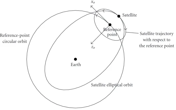
To describe the kinematics of coplanar configurations, it is useful to consider the relative motion of a satellite moving on an orbit of given eccentricity and semimajor axis, with respect to a reference point describing a reference trajectory. The selected reference trajectory is a Keplerian circular or-bit lying in the satellite oror-bital plane, sharing the same mean motion (n) of satellite elliptical orbit, hence the two orbits exhibit the same semimajor axes (i.e., the semimajor axis of the elliptical orbit is equal to the circular orbit radius) and orbital periods (T).

Now, letxozo be an orbiting reference frame (ORFO, in

the following the subscriptOwill refer to the reference or-bit) whose origin coincides with the position of the reference point (xo-axis directed as the velocity vector,zo-axis in nadir

direction); assuming that mean anomalyMinitial value is

M≡ −ω+θ0, (18)

whereθ0is the initial value of the true anomaly of the refer-ence point with respect to the ascending node, the following equations can be derived by a series expansion in powers of eccentricity [23]:

xo(t)=2aesin

nt+θ0−ω

+ae 2

4 sin 2

nt+θ0−ω

+ae 3

24

7 sin 3nt+θ0−ω

−9 sinnt+θ0−ω

+Oe4_,

zo(t)=aecos

nt+θ0−ω

+ae 2

2

1−cos 2nt+θ0−ω

+3 8ae

3_cosnt+θ 0−ω

−cos 3nt+θ0−ω

+Oe4_,

(19)

wheretis the time elapsed since initial instant. By truncating the series at first order in eccentricity, the satellite trajectory with respect to the reference point is an ellipse whose cen-ter coincides with the reference point and with principal axes directions coincident withxozodirections. In particular,

respec-Reference-point circular orbit

Earth

Satellite Reference

point

Satellite elliptical orbit

Satellite trajectory with respect to the reference point xo

zo

Figure4: Satellite and reference point motion, plotted with satellite at apogee (not in scale for clarity).

tively. The angle in the ellipse plane varies with a constant rate (coincident with the satellite mean motion), in oppo-site direction with respect to the orbital motion, as shown in Figure 4.

If the assumption (18) is discarded, the series expan-sion is more complicated, but similar concluexpan-sions can be ob-tained, with the approximated ellipse translated and rotated with respect toxozoaxes.

Obviously, the elliptical approximation is more and more inaccurate when orbit eccentricity increases [23], which is not our case.

4.1. Cartwheel

The interferometric cartwheel, introduced and patented by Massonnet [8, 9], is basically a formation of passive mi-crosatellites forming an orbiting cartwheel in the orbital plane of an active one, thanks to adequate differences in perigee positions and true anomalies synchronization. All satellites exhibit the same orbit eccentricity and semimajor

axis. Multiple along-track and vertical baselines can be si-multaneously achieved, although varying along the orbit. Obviously, increasing the number of microsatellites, forma-tion duty cycle can be greatly improved [24]. This is not ap-plicable to COSMO-BISSAT formation, since only two plat-forms are available. However, it is interesting to investigate limits and potentialities of cartwheel configuration also in this case.

First of all, considering that COSMO is in sun-synchronous low-eccentricity orbit, a Keplerian circu-lar orbit with radius equal to COSMO semimajor axis (6997.940 km) has been selected as reference. Hence, COSMO and BISSAT form a cartwheel around the circu-lar trajectory, as a consequence of their equal eccentricity (Figure 5).

From the linearized equations of motion (19), in order to obtain that the two satellites occupy the same positions in the orbiting reference frame, with a time delay∆t, we must impose

MC(0)=θ0−ωC

MB(0)=θ0−ωB

=⇒MC(0)−MB(0)=ωB−ωC=γ=n·∆t=f ·π. (20)

Considering the trajectories in the orbiting reference frame (for the sake of simplicity, it has been assumed that att =

0, COSMO is at its perigee), γ is the angular separation between the satellites (Figure 6), and it can be expressed by multiplying the reference orbit mean motion times the required time separation between the satellites, or, more

conveniently for constellation tuning, as a fraction (f) of

π.

Reference circular orbit COSMO

BISSAT

COSMO orbit

BISSAT orbit BISSAT

perigee

xo

zo

XC ZC

ωB=ωC+γ

νB(0)=νC(T−∆t)

Figure 5: Geometry adopted to describe the COSMO-BISSAT cartwheel (plotted with COSMO at perigee and not in scale for clar-ity).

20 15 10 5 0

−5

−10

−15

−20

xo(km)

−10

−8

−6

−4

−2 0 2 4 6 8 10

zo

(km)

COSMO att=0 BISSAT att=0

γ

Figure6: Motion in the ORFO.

Figure 8andTable 2summarize the main performances achievable with this configuration.

It is worth noting that adequate vertical baselines can be achieved almost along the whole orbit (only polar regions are excluded).

4.2. Alternative coplanar configurations

Two alternative solutions for baseline formation, still based on coplanar orbits, are achievable by orbiting COSMO and BISSAT with different eccentricities and equal argument of perigee and mean anomaly (Figure 9), or by choosing a

5826 5000 4000

3000 2000

1000 0

Time (s)

1 0.9 0.8 0.7 0.6 0.5 0.4 0.3 0.2 0.1 0

Orbit fraction

−4

−2 0 2 4

Baseline

co

mponents

(km)

Along-track baseline Vertical baseline

Figure7: Interferometric baseline components forf =0.0833 as a function of time along one orbit.

180 160 140 120 100 80 60 40 20 0

Perigee separation (◦) 0

0.1 0.2 0.3 0.4 0.5 0.6 0.7 0.8 0.9 1

Or

bit

fr

actions

adeq

uat

e

for

X

TI

and

A

TI

XTI ATI

Figure8: COSMO-BISSAT cartwheel performance as a function of

γ, expressed in terms of fraction of orbit where satisfactory baselines are achieved.

trajectory for BISSAT which differs from the COSMO one only in the argument of perigee (Figure 10).

In these cases, the two satellites will not move on the same ellipse, with respect to the ORFO. In the first

COSMO BISSAT xo

zo

XC ZC

ωB=ωC

Figure9: Orbits with different eccentricities (not in scale for clar-ity).

dimensions, will be translated onxo-axis (this can be shown

performing the series expansion in powers of eccentricity without the assumption (18), and supposingM(0)−θ0+ω small).

From the relative motion point of view, having two or-bits which differ only in perigee argument is equivalent to put the two satellites on the same orbit, with a short time separation: the ORFO coordinates of the ellipse origin are,

in fact, asin[M(0) +ω−θ0] and a−acos[M(0) +ω−

θ0]. The along-track baseline component is constant, and to achieve an adequate vertical baseline, a large along-track separation (> 50 km) is needed. As a consequence, this configuration can be used only for ATI; in particular, ifωB∈

[89.9988◦, 89.9994◦], the entire orbit can be exploited. In the case of different eccentricities, from the baselines’ point of view, a different behavior from the cartwheel is ex-hibited. In fact, as it is evident fromFigure 11(still supposing that att=0, COSMO is at its perigee), the vertical spacecraft separation is maximum at the poles and minimum at the as-cending/descending nodes, while the along-track baseline is maximum at the nodes.

The achievable performances are quantitatively similar to the cartwheel ones, as shown inFigure 12andTable 3, and it is interesting to point out the difference in useful latitude intervals consequent to the different trend of baseline com-ponents.

5. TANDEM FLIGHT IN PENDULUM CONFIGURATION

The wording “pendulum,” introduced in [7,10,25], refers to orbits separated in the right ascension of the ascending node and, if required, with different inclinations and true anoma-lies (Figures2and13).

COSMO

BISSAT xo

zo

XC ZC

ωC ωB

Figure10: Orbits with different arguments of perigee (not in scale for clarity).

5826 5000 4000

3000 2000 1000

0

Time (s)

1 0.9 0.8 0.7 0.6 0.5 0.4 0.3 0.2 0.1 0

Orbit fraction

−4

−2 0 2 4

Baseline

co

mponents

(km)

Along-track baseline Vertical baseline

Figure11: Interferometric baseline components along one orbit, foreB=1.5·10−3.

In order to have “J2-invariant” orbits [26,27], it is appro-priate to choose equal inclinations.

Table2: Cartwheel phasings which maximize percentage of orbit adequate for XTI and ATI and consequent latitude intervals during as-cending/descending phases.

Interferometric configuration XTI ATI

Perigee separation (◦_{) 20.74 0.52}

Time separation (s) 335.6 8.41

Minimum distance (km) 2.97 0.0749

Orbit fraction (%) 97.94 66.64

[82.13, 78.49] desc. [82.13, 29.41] desc. Latitude intervals (◦) [75.56,−78.38] desc. [−30.02,−29.52] desc/asc.

[−75.45, 82.13] asc. [29.91, 82.13] asc.

thus, recallingxyzas the orbiting reference frame whose ori-gin coincides with COSMO position, and assuming that at

t=0, COSMO is at the ascending node, the following equa-tion can be derived to express BISSAT posiequa-tion with respect to COSMO:

  

x(t)

y(t)

z(t)   ∼=

  

a(∆ν+∆Ωcosi)

asini∆Ωcos(nt) 0

 

. (21)

It is worth noting that cross-track baseline is formed in the horizontal plane and depends only on∆Ω, while along-track baseline is constant and, for the considered value of sun-synchronous inclination, depends above all on ∆ν. In this case, the two spacecrafts move along almost parallel trajecto-ries, for short orbital segments, whereas the horizontal base-line component varies as a function of latitude over longer periods [28]. In particular, from the second component of (21), the optimal value of ∆Ω for XTI can be estimated by imposing ymax = Bymax, resulting ∆Ω = 0.0163◦. The numerical simulations, performed taking into account the slight eccentricities of the orbits, confirmed this estimate, as shown inFigure 14. In order to get an adequate along-track separation,∆ν= −5·10−3◦_{has been assumed.}

As for along-track interferometry is concerned, with this configuration we can achieve an ideal observation geometry. In fact, it must be considered that Earth rotation prevents two antennas, which move on the same orbit with a time sep-aration∆t, from having the same viewing geometry.

As shown in [21], imposing the conditions (ΩEis Earth

rotation rate)

ΩB−ΩC

ΩE−Ω˙ = νC−νB

˙

M+ ˙ω =∆t, (22)

the two antennas will exhibit the same trajectory, with re-spect to an Earth-fixed, rotating reference frameFigure 15. Obviously, the two satellites will have the same ground track too, thus allowing coverage geometry adequate for ATI.

Considering, for the sake of simplicity, the unperturbed case (n=µ/a3₎

ΩB−ΩC

ΩE = νC−νB

n =∆t, (23)

2 1.8 1.6 1.4 1.2 1 0.8 0.6 0.4

×10−3 BISSAT eccentricity

0 0.1 0.2 0.3 0.4 0.5 0.6 0.7 0.8 0.9 1

Or

bit

fr

actions

adeq

uat

e

for

X

TI

and

A

TI

XTI ATI

Figure12: Configuration performances as a function of BISSAT ec-centricity, expressed in terms of fraction of orbit where satisfactory baselines are achieved.

and choosing ∆t = 10 milliseconds (corresponding to an along-track baseline of about the order of 75 m, which allows to evaluate aV rmax of the order of 1.56 m/s), the following values are derived:

ΩB−ΩC=4.18·10−5◦,

νC−νB=6.18·10−4◦. (24)

Relevant results are summarized inTable 4, showing the excellent ATI performance achievable with pendulum tan-dem configuration.

Table3: BISSAT eccentricities which maximize percentage of orbit adequate for XTI and ATI and consequent latitude intervals during ascending/descending phases.

Interferometric configuration XTI ATI

BISSAT eccentricity 7.62·10−4 _1.169·10−3

Minimum distance (km) 2.89 0.0749

Orbit fraction (%) 97.92 66.61

[82.13, 1.94] desc.

[59.02,−59, 03] desc. [−59.06, 58.99] asc. Latitude intervals (◦) [−1.77,−1.81] desc/asc.

[1.90, 82.13] asc.

Equator

Figure13: Geometry of pendulum configuration.

of different eccentricities. So, if interferometric coverage is requested at a particular latitude with a given effective base-line, proposed orbits can fulfill it either by tuning the design parameters for a certain configuration or by combining dif-ferent configurations (e.g., combining cartwheel or pendu-lum with a difference in eccentricity). Of course, identified orbital configuration will be less effective, or useless in the worst case, at other latitudes.

On the other hand, one can think of using different or-bital configurations to achieve different interferometric pairs on a given area, to combine the advantages of large and small baseline (accuracy and easier phase unwrapping), though there will be some unavoidable temporal gap between the acquisitions. To this end, optimal strategies for orbit trans-fer, accounting for spacecraft resources, will be addressed by further studies.

As a matter of fact, ATI can be achieved in a more sta-ble fashion along the orbit, although with critically short baselines, whereas XTI baselines can be achieved with safer orbital configurations, although criticality arises in this case from continuous baseline variations.

6. CONSIDERATIONS ON THE STABILITY OF COPLANAR AND PENDULUM CONFIGURATIONS So far, orbit fractions, where satisfactory baselines are achieved, have been evaluated assuming unperturbed mo-tion. However, one must consider orbital perturbations to

0.1 0.09 0.08 0.07 0.06 0.05 0.04 0.03 0.02 0.01 0

Di_fference in right ascension of the ascending node (◦) 0

0.1 0.2 0.3 0.4 0.5 0.6 0.7 0.8 0.9 1

Or

bit

fr

action

adeq

u

at

e

for

X

T

I

Figure14: Pendulum performance as a function of∆Ω, expressed in terms of fraction of orbit where a satisfactory XTI baseline is achieved.

estimate the long period evolution of designed configura-tions. To this end, it must be considered the boundary con-straint deriving from the fact that we are not dealing with an original formation, on the contrary BISSAT strategies for baseline control will strongly depend on the operative sched-ule of the active satellite, which, as previously underlined, cannot be modified.

In this context, it is evident that, being a dual-use constel-lation aimed at monitoring and surveillance for commercial, scientific, and military applications, COSMO will be char-acterized by an accurate orbit control that counteracts the effects of drag, solar radiation pressure, and third-body ac-celerations. Regarding these perturbations, it can be foreseen that, for BISSAT, the firing sequence and the propellant ex-pense should be similar to COSMO ones. It is expected that this is particularly true if the same bus of COSMO will be adopted for BISSAT.

Table4: Pendulum configurations which maximize percentage of orbit adequate for XTI and ATI and consequent latitude intervals during ascending/descending phases.

Interferometric configuration XTI ATI

∆Ω(◦_{) 0.0162 4.18·10}−5◦

∆ν(◦_{) −5·10}−3 _−6.18·10−4◦

Minimum distance (km) 0.879 0.075

Orbit fraction (%) 97.93 100

Latitude intervals (◦) [81.92,−81, 91] desc. All the achievable latitudes [−81.92, 81.91] asc.

Z

X

Y COSMO

orbit

BISSAT orbit

COSMO

BISSAT ΩE

ΩB ΩC

∆Ω i

i

∆ν

Figure15: Along-track interferometer: positions at the ascending node.

As for nonspherical Earth effects are concerned, COSMO argument of perigee will be kept in a certain range around 90◦, by nullifying the J2 induced precession of the line of apsides. This effect is moderate since COSMO orbit is frozen. From formation keeping point of view, the configuration with different eccentricities is the only one that is not J2 -invariant. However, differential secularJ2effects on the evo-lution of the interferometric baseline are negligible in the considered case, as it can be seen in Figures16and17, where relative trajectory is reported foreB =0.00140, and for 450

COSMO nodal periods. In this simulation, onlyJ2secular ef-fects have been considered (without any correction): it can be seen that the growth of baseline horizontal component is so slow that, after one month, the secular value is still smaller than 5 m.

This is due to the fact that, for near circular orbits, ˙Ω, ˙

ω, and ˙Mare much more sensitive to∆ithan to∆e(in fact,

∂Ω˙/∂e|e=0=∂M/∂e˙ |e=0=∂ω/∂e˙ |e=0=0), so the differences in mean anomaly, argument of perigee, and right ascension of the ascending node are, in the considered case, of order 10−3◦_/y.

As for latitude coverage is concerned, it is obvious that if the precession of the line of apsides were not counteracted,

the latitude intervals in which interferometry is possible, with certain baselines, would be altered. As previously stated, argument of perigee control is envisaged in COSMO opera-tive schedule because of strict repetiopera-tiveness requirements. As for BISSAT, only in the pendulum case, passive satellite or-bit is frozen; in the cartwheel case, for example, argument of perigee control will be more onerous, leading to a (presumi-bly slight) difference in fuel consumption.

To summarize, pendulum is the stablest configuration, followed by cartwheel (not frozen) and∆e(notJ2-invariant).

7. CONCLUSIONS

This paper focused on orbital configurations adequate for complementing the Italian COSMO SAR constellation with interferometry. A fifth satellite has been considered that, thanks to expectable mass reductions consequent to a sim-plified passive payload, could offer additional maneuvers ca-pabilities, thus allowing, as an example, mission changes from along-track to cross-track interferometry, depending on particular users’ requirements. To this end, further stud-ies will be addressed to characterize optimal strategstud-ies for or-bit transfer. Enlarged maneuvers capabilities could also al-low flight of the fifth satellite in formation with a varying COSMO spacecraft, thus achieving an overall reliability im-provement. In addition, it is worth noting that the proposed idea of a passive satellite can be fulfilled by considering only recurrent costs or by using most of the engineering model of the spacecraft. On the other hand, the weight, volume, and cost advantages connected with the use of a simplified, receiving-only payload could allow additional remote sens-ing systems to be embarked, such as a laser altimeter or an atmospheric profiler which could take advantage of the COSMO terminator orbit too.

4 3 2 1 0

−1

−2

−3

−4

x(along-track separation) (km)

−2

−1.5

−1

−0.5 0 0.5 1 1.5 2

z

(r

adial

separ

ation)

(km)

2.04

2.03

2.02

2.01

2

1.99

1.98

1.97

1.96

1.14

1.145

1.15

1.155

1.16

1.165

1.17

1.175

1.18

1.185

1.19

1st nodal period 450th nodal period

Figure16: In-plane relative trajectory, plotted foreB=0.00140 and 450 nodal periods.

50th nodal period

150th nodal period

250th nodal period

350th nodal period

450th nodal period Time

−5

−4

−3

−2

−1 0 1 2 3 4 5

y

(hor

iz

ontal

distanc

e)

(m)

Figure17: Secular growth of baseline horizontal component, plot-ted foreB=0.00140.

ascending node and true anomaly separations adequate to match Earth rotation. Regarding cross-track interferometry, developed model allowed identification of several solutions which enable coverage for more than 90% of the orbit. Fur-thermore, it was shown that by tuning orbital parameters such as perigee, ascending node, anomaly separation, or or-bit eccentricity, it is possible to set the latitude interval in which cross-track SAR interferometry is carried out with se-lected horizontal or vertical baseline.

ACKNOWLEDGMENT

This paper has been carried out with financial support from the Italian Space Agency and Ministry for Education, Univer-sity and Research.

REFERENCES

[1] F. Caltagirone, G. Angino, A. Coletta, F. Impagnatiello, and A. Gallon, “COSMO-SkyMed program: Status and perspectives,” inProc. 3rd International Workshop on Satellite Constellations and Formation Flying, pp. 11–16, Pisa, Italy, February 2003. [2] F. Caltagirone, P. Spera, G. Manoni, and L. Bianchi,

“COSMO-SkyMED: A dual use earth observation constella-tion,” inProc. 2nd International Workshop on Satellite Constel-lations and Formation Flying, pp. 87–94, Haifa, Israel, Febru-ary 2001.

[3] A. Moccia, N. Chiacchio, and A. Capone, “Spaceborne bistatic synthetic aperture radar for remote sensing applications,” International Journal of Remote Sensing, vol. 21, no. 18, pp. 3395–3414, 2000.

[4] M. D’Errico and A. Moccia, “Attitude and antenna pointing design of bistatic radar formations,”IEEE Trans. Aerosp. Elec-tron. Syst., vol. 39, no. 3, pp. 949–960, 2003.

[5] H. A. Zebker and J. Villasenor, “Decorrelation in interfer-ometric radar echoes,”IEEE Trans. Geosci. Remote Sensing, vol. 30, no. 5, pp. 950–959, 1992.

[6] G. Krieger, H. Fiedler, J. Mittermayer, K. Papathanassiou, and A. Moreira, “Analysis of multistatic configurations for space-borne SAR interferometry,”IEE Proceedings - Radar, Sonar and Navigation, vol. 150, no. 3, pp. 87–96, 2003.

[7] G. Krieger, M. Wendler, H. Fiedler, J. Mittermayer, and A. Moreira, “Performance analysis for bistatic interferometric SAR configurations,” inProc. IEEE International Geoscience and Remote Sensing Symposium (IGARSS ’02), vol. 1, pp. 650– 652, Toronto, Canada, June 2002.

[8] D. Massonnet, “Capabilities and limitations of the interfero-metric cartwheel,”IEEE Trans. Geosci. Remote Sensing, vol. 39, no. 3, pp. 506–520, 2001.

[9] D. Massonnet, “The interferometric cartwheel: a constellation of passive satellites to produce radar images to be coherently combined,”International Journal of Remote Sensing, vol. 22, no. 12, pp. 2413–2430, 2001.

Aperture Radar (EUSAR ’02), pp. 29–32, Cologne, Germany, June 2002.

[11] H. A. Zebker, T. G. Farr, R. P. Salazar, and T. H. Dixon, “Map-ping the world’s topography using radar interferometry: the TOPSAT mission,”Proc. IEEE, vol. 82, no. 12, pp. 1774–1786, 1994.

[12] M. D’Errico, A. Moccia, and S. Vetrella, “High frequency ob-servation by GTM antenna range beam steering,”EARSeL Ad-vances in Remote Sensing, vol. 3, no. 1-IX, pp. 60–69, 1994. [13] R. Gens and J. L. van Genderen, “SAR interferometry—

issues, techniques, applications,”International Journal of Re-mote Sensing, vol. 17, no. 10, pp. 1803–1836, 1996.

[14] P. A. Rosen, S. Hensley, I. R. Joughin, et al., “Synthetic aper-ture radar interferometry,”Proc. IEEE, vol. 88, no. 3, pp. 333– 382, 2000.

[15] A. Moccia, S. Esposito, and M. D’Errico, “Height measure-ment accuracy of ERS-1 SAR interferometry,”EARSeL Ad-vances in Remote Sensing, vol. 3, no. 1, pp. 94–108, 1994. [16] F. K. Li and R. M. Goldstein, “Studies of multibaseline

space-borne interferometric synthetic aperture radars,”IEEE Trans. Geosci. Remote Sensing, vol. 28, no. 1, pp. 88–97, 1990. [17] E. Rodriguez and J. M. Martin, “Theory and design of

in-terferometric synthetic aperture radars,” IEE Proceedings F, Radar & Signal Processing, vol. 139, no. 2, pp. 147–159, 1992. [18] A. Moccia and S. Vetrella, “A tethered interferometric

syn-thetic aperture radar (SAR) for atopographic mission,”IEEE Trans. Geosci. Remote Sensing, vol. 30, no. 1, pp. 103–109, 1992.

[19] R. Bamler and P. Hartl, “Synthetic aperture radar interferom-etry,”Inverse Problems, vol. 14, no. 4, pp. R1–R54, 1998. [20] R. Romeiser, M. Schw¨abisch, J. Schulz-Stellenfleth, et al.,

“Study on concepts for radar interferometry from satellites for ocean (and land) applications (KoRIOLiS),” Final Report, University of Hamburg, Hamburg, Germany, 2002.

[21] A. Moccia and G. Rufino, “Spaceborne along-track SAR inter-ferometry: performance analysis and mission scenarios,”IEEE Trans. Aerosp. Electron. Syst., vol. 37, no. 1, pp. 199–213, 2001. [22] V. A. Chobotov, Ed., Orbital Mechanics, AIAA Education Series, American Institute of Aeronautics and Astronautics, Washington, DC, USA, 1991.

[23] A. Miele and M. D’Errico, “A relative orbital motion model oriented to formation design,” in Proc. 3rd International Workshop on Satellite Constellations and Formation Flying, Pisa, Italy, February 2003.

[24] D. Massonnet, E. Thouvenot, S. Ramongassi`e, and L. Phalip-pou, “A wheel of passive radar microsats for upgrading exist-ing SAR projects,” inProc. IEEE International Geoscience and Remote Sensing Symposium (IGARSS ’00), vol. 3, pp. 1000– 1003, Honolulu, Hawaii, USA, July 2000.

[25] J. Mittermayer, G. Krieger, A. Moreira, and M. Wendler, “In-terferometric performance estimation of the in“In-terferometric cartwheel in combination with a transmitting SAR-satellite,” in Proc. IEEE International Geoscience and Remote Sensing Symposium (IGARSS ’01), vol. 7, pp. 2955–2957, Sydney, NSW, Australia, July 2001.

[26] H. Schaub, S. R. Vadali, J. L. Junkins, and K. T. Alfriend, “Spacecraft formation flying control using mean orbit ele-ments,” inProc. AAS/AIAA Astrodynamics Specialists Confer-ence, Girdwood, Alaska, August 1999, Paper No. AAS 99-310. [27] H. Schaub and K. T. Alfriend, “J2 invariant relative orbits for spacecraft formations,”Celestial Mechanics and Dynami-cal Astronomy, vol. 79, no. 2, pp. 77–95, 2001.

[28] A. Moccia, S. Vetrella, and M. D’Errico, “Twin satellite or-bital and doppler parameters for global topographic map-ping,”EARSeL Advances in Remote Sensing, vol. 4, no. 2-X, pp. 55–66, 1995.

A. Mocciahas been a Professor of aerospace servosystems at the Faculty of Engineer-ing, University of Naples, Naples, Italy, since 1990. His research activities deal with aerospace high-resolution remote-sensing systems, mission analysis, design, and data processing, as well as aerospace systems dy-namics and control. He has been a mem-ber of national and international commit-tees and working groups (ASI, NASA, ESA,

UE, CIRA, EARSA eL, MIUR) and principal or coinvestigator of several national and international research programs. He is the au-thor or coauau-thor of more than 100 scientific papers, and gained several references in international journals. Since 1975, he has held several grants and contracts from the National Research Council, University of Naples, Italian Space Agency, ESA, Italian Ministry for Education, University and Research, Alenia Spazio, Telespazio, and Technapoli. Since 2001, he has been the Chairman of the Ph.D. School in Aerospace Engineering at the University of Naples and President of CORISTA, Consortium for Research on Aerospace Remote Sensing Systems, a nonprofit research consortium among Universities of Naples and Bari, Alenia Spazio, and Laben.