Bootstrap Nonlinear Regression Application in a Design of an Experiment Data for Fewer Sample Size

(1)

INTERNATIONAL JOURNAL OF RESEARCH (IJR) E-ISSN: 2348-6848, P- ISSN: 2348-795X VOLUME 2, ISSUE 2, FEB. 2015

AVAILABLE AT HTTP://INTERNATIONALJOURNALOFRESEARCH.ORG

Bootstrap Nonlinear Regression Application in a Design of an

Experi-ment Data for Fewer Sample Size

Bello, Oyedele Adeshina1_{; Bamiduro, Timothy Adebayo}2_{; Chuwkwu, Unna Angela} 2_&

Osowole, Oyedeji Isola2

1. Department.of StatisticsFederal University of Technology, Minna, Niger State, Nigeria.

[email protected]

2. Department of Statistics University of Ibadan, Nigeria.

[email protected]

Abstract—

This paper reports on application of bootstrap nonlinear regression method to a design of an ex-periment dataset with fewer exex-perimental runs. Design with desired properties was augmented and verified using graphical techniques. The augment-ed design with the desiraugment-ed properties benefitaugment-ed the accuracy of the approximated function used.

The computation power of R-language and SAS for computing nonlinear function and bootstrap was also compared.

Keywords—

Bootstrap non-linear regression; Gauss Newton-Bootstrap Re-Sampling Method; Sample size; Data visualization (EDA); Graphical technique; R

programming language and SAS

Introduction

The beauty of statistics is in its ability to obtain an

approximation for the function ( f ), that is able

to describe a phenomenon of interest, but often time some phenomenon generate little or no data (insufficient information or sample size) which makes it difficult to obtain sufficient, efficient and robust estimates. Nevertheless, finding an ap-proximate function to describe the relating varia-bles in such phenomenon is still of interest. Therefore, we need to look for a way around the problem.

1.1The Problem of Data Sufficiency and the

Cost of An Experiment

The availability of sufficient information or sam-ple size about a phenomenon is not always at the researcher luxury. Some phenomenon could

(2)

sud-INTERNATIONAL JOURNAL OF RESEARCH (IJR) E-ISSN: 2348-6848, P- ISSN: 2348-795X VOLUME 2, ISSUE 2, FEB. 2015

den movement of the galaxies or earth crust in away it has never done before, the little jot of in-formation from such newly discovered phenome-non can be mimic or better still simulated to gen-erate a much larger datasets. But simulation can be highly prone to error because most of the simulation methods tell us little or nothing about the distribution of such simulated data, if at all it does, does the simulated data conform to the true distribution of the simulated phenomenon. This work shall prefer to re-sample such token infor-mation or sample to give birth to a much larger sample size using the bootstrap re-sampling method. The name “bootstrap” incidentally con-veys the impression of “something for nothing” where statisticians idly re-sampling from their samples (F.W. Scholz, 2007). Bootstrap re sam-pling method cancelled out the problem of large variance which usually arises when modelling with small set of samples.

1.2 Data Visualization:

The first step to computing in statistics is to look at your data and ask researchable questions on it. The method of data visualization can aid in look-ing indept into the data so as to be able to ask necessary questions about the phenomenon of study. The failure of taking advantage of the ex-ploratory data analyses (EDA) or any other meth-od of data visualization usually results to using a correct answer to answer a wrong question. The method of data visualization helps to suggest the possible relationship existing between variables involved and in generality a close and relevant function can be approximate. According to Julian J. Faraway (2002) “Statistics starts with a prob-lem, continues with the collection of data,

pro-ceeds with the data analysis and finishes with conclusions. It is a common mistake of inexperi-enced Statisticians to plunge into a complex anal-ysis without paying attention to what the objec-tives are or even whether the data are appropriate for the proposed analysis. Look before you leap!” One important way to look before leaping is to visualize your data so you don’t prescribe a linear function for a non-linear relationship.

1.2Exploratory Data Analysis (EDA):

This method of analysis uses visualization tools and computes synthetic descriptors. EDA is re-quired at the beginning of the statistical analysis of multidimensional data, in order to get an over-view of the data, transform or recode some varia-bles orient further analyses (Daniel Borcard et al, 2011). Data visualization helps to detect outliers, spotting local structures, systematic errors in the data, skewed or unusual distributions trends, clus-ters, and for evaluating modelling output and pre-senting results. Note, deciding on which graphics to use is often research and researchers view de-pendent. Most importantly, EDA is a major way of suspecting a nonlinear dataset in a regression problem.

1.3Exactness VS. Approximate Function-The

Avoidance Of Nonlinear Problems

(3)

In a linear model we have had to ensure that the normal equations, which are the first derivatives of the objective function with respect to the coef-ficients, were independent of the coefficients. This constraint has precluded us from using a wealth of biologically realistic model forms. The messiness is unavoidable; the avoidance of non-linear is basically because of its numerous numer-ical iterations and being highly computer-intensive in solving the problem.

However, it is arguably better to get an approxi-mate answer to a meaningful question than to get an exact answer to an approximation to a mean-ingful question (Tukey, 1962). Despite the passive challenges to solving a nonlinear problem we should choose model forms that genuinely repre-sent the phenomenon under study. (See Andrew P. Robinson and Jeff D. Hamann; Forest Analytics with R- An Introduction pg. 199-203 for details). Advantages of Nonlinear Models

Nonlinear models are often derived on the basis of physical, chemical or biological considerations, also, from differential equations, and have justifi-cation within a quantitative conceptualization of the process of interest.

The parameters of a nonlinear model usually have direct interpretation in terms of the process under study.

Constraints can be built into a nonlinear model easily and are harder to enforce for linear models. Truly, fitting a nonlinear regression model to data is slightly cumbersome but we would usually pre-fer such a model whenever possible, rather than to its alternative, perhaps less realistic linear model.

2 METHODOLOGY

Considering;

y= f(x)β +ε (1)

Where x=(x₁_,x₂_,...,x_k), β s is the coefficient

estimates,

ε

(error term) ~ N (0; 1) and

independ-ent. f is the function that describes the form in

which the response and the input variable are re-lated, its mathematical form is not known in prac-tice. It is often approximated within the experi-mental region.

2.1 _{The Design}

Factorial Design is a class of orthogonal design used for fitting first order model, this work makes use of factorial design with four levels. The cen-tral composite design was used to fit the second order. Fitting second order model also means augmentation of additional points to the initial first order design. The full factorial runs with na = 2k points on the axis of each factor at a distance from the center of the design.

The center runs n0(0,0...,0) without replication. The total number of runs N=nf + na + no.

The practical deployment of a CCD often arises through sequential experimentation, as that is, when a factorial design has been used to fit a first-order model, this model has exhibited lack of fit, and the axial runs are then added to allow the quadratic terms to be incorporated into the model. There are two parameters in the design that must

be specified: the distance α of the axial runs from

the design centre and the number of center points n0. See Appendix III for the constructed designs

The Desired Properties

Orthogonality: A design D is said to be orthogonal if the matrix XX is diagonal, where X is the

mod-el matrix ofy= Xβ +ε . The elements of X′X

(4)

Rotatability: A design D is said to be rotatable if

the prediction variance

) ( ) ' ( )] ( ˆ

[ 2 1

x f X X x

y

Var =δ − is constant at all

points that are equidistant from the design centre. The prediction variance remains unchanged under any rotation of the coordinate axes.

[1] Uniform Precision: A rotatable design is said

to have the additional uniform precision prop-erty if Var [ yˆ (x)] at the origin is equal to its value at a distance of one from the origin. This helps in producing some stability in the prediction variance in the vicinity of the de-sign centre. For details on RSM, Dede-sign and properties See; Andre I Khuri et al (2010), Khuri, AI, Cornell (1996) , Bello O.A. (2014). “Modeling Cassava Yield: A Response

Surface Methodology Approach.”,

Un-published M.Sc Thesis, University of Ibadan Nigeria, and Bello O. A. ( 2014) International Journal on Computational Sciences & Appli-cations (IJCSA) Vol.4, No.3, June 2014, 63 for details.

3 THE INVERSE POLYNOMIAL – A NONLINEAR

FUNCTION

The Inverse Polynomial –A Nonlinear Function

The general forms of Inverse Polynomials of (Nelder, 1966; Nduka, 1994; Holger Dette, 2007) are family of non-linear function and it is intrinsi-cally nonlinear.

) ...

( 1

1 2

2 1 0 1 1

− − =

=

+ + + + =

_∏

∏

p

i i p i

i i i k

i k

i i

x x

x q

x

β β

β

β ₍₂₎

Where, k = number of factors q = the yield per unit area.

p = number of levels of factor i.

Intrinsically Nonlinear Model: This is when there is nonlinearity in parameters and linearity cannot be achieved through transformation.

The First Order Model;

1 2 1 00 1 2 10 1 1 01 11 1

)

( −

− −

− ₌ ₊ ₊₊ ₊₊

x x x

x

y β β β β (3)

The Second Order Model;

1 2 1 00 1 2 1 20 1 1 2 02 1 2 10 1 1 01 11 1

)

( −

− −

− ₌ ₊ ₊ ₊ ₊ ₊

x x x

x x

x

y β β β β β β

(4)

For details on properties of the nonlinear model [See Nduka, E. C. 1994, 1997].

3.1 _{Parameter Estimation Of A Nonlinear}

Function

When the normal equation is extremely difficult to solve, it may happen to have multiple solution to multiple stationary values of function of S(θ). It is said to have no closed form solution. Thereby the procedure of iterative method must be ap-proached in order to manoeuvre the mathematical intractable problem (Bello O.A. 2014).

3.2 _{Nonlinearity of the Model.}

Considering the parameterθ, the estimate (θˆ ) of

θ is obtained by differentiating equation S(θˆ ) and equated to zero, resulting to p-1 normal equa-tions. Also, considering the nonlinear model in (4). The sum of square error for our nonlinear model follows the definition;

2

1

] ) , ( [ )

(

∑

=

− =

n

i

j i i f x

y

S θ θ (5)

2 1 11 2 1 02 2

2 20 2 01 1 10 2

1

x x x

x x

x y

x x

oo β β β β β

β + + + + +

=

Taking inverse of −1

y

1 1 2 1 00 1 1 2 02 1 2 1 20 1 2 10 1 1 01

11 ( ) ]

[ − − − − − −

+ +

+ + +

= x x xx x x x x

y β β β β β β

j

j θ

β =

Let

1 1 2 1 00 1 1 2 02 1 2 1 20 1 2 10 1 1 01

11 ( ) ]

[ ) ,

( − − − − − −

+ +

+ + +

= x x xx x x xx

x

f θ θ θ θ θ θ θ

(5)

Recall the sum of square

) , ( ) ( , ) ˆ ( )

(θ ₁ y y 2 E y f xθ

S n

i − =

=

∑

=

0 ) (

E ε =

given , thereby;

] ) ) ( ( [ )

( 1 1

2 1 00 1 1 2 02 1 2 1 20 1 2 10 1 1 01 11 1 − − − − − − = + + + + + −

=∑y x x xx x x xx

S i n i θ θ θ θ θ θ θ (7)

The estimation of parameters θj is obtained by

differentiating equation S(θ) for ψij equated to

zero and solving for the θ_s_' respectively.

j i n i x f x x x x x x x x y S θ θ θ θ θ θ θ θ θ ∂ ∂ + + + + + − = − − − − − − = ∑ (, ) ] ) ) ( ( [ )

( 1 1

2 1 00 1 1 2 02 1 2 1 20 1 2 10 1 1 01 11 1 (8)

When the normal equation contains parameters that are depending on each other, we have a non-linear problem which can be solved iteratively using computer software.

) 9 ( 0 ] ) ) ( )][ , ( [ 0 ] ) ) ( )][ , ( [ 0 ) ]( ) ) ( )][ ( [ 1 2 2 1 1 2 1 00 1 1 2 02 1 2 1 20 1 2 10 1 1 01 11 1 1 1 2 1 2 1 00 1 1 2 02 1 2 1 20 1 2 10 1 1 01 11 1 2 1 2 1 1 2 1 00 1 1 2 02 1 2 1 20 1 2 10 1 1 01 11 4 4 4 4 4 4 4 4 4 4 4 4 4 4 4 4 4 3 4 4 4 4 4 4 4 4 4 4 4 4 4 4 4 4 4 2 1 equation normal The n i i i n i i i n i i i x x x x x x x x x x f y x x x x x x x x x x f y x x x x x x x x x x x f y = + + + + + − = + + + + + − = + + + + + − − − = − − − − − − = − − − − − − − − = − − − − − ∑ ∑ ∑ θ θ θ θ θ θ θ θ θ θ θ θ θ θ θ θ θ θ θ θ θ

The normal equation in (9) is produced by the

dif-ferentiation of S(θ) which involved model

param-eters that are nonlinear in relationship, the equa-tion is mathematically intractable, cannot be solved analytically but could only be solved itera-tively.

3.3 _{The Gauss Newton Method.}

Choice of iterative algorithm is to minimize the sum of square error of the parameter estimates. The nonlinear least square surface is approximat-ed basapproximat-ed on the linear approximation, until no fur-ther improvement can be made, using the result of

linear least squares in successive stages. At that point of no further improvement in decrease of sum of squared error, we say the steps have con-verged to a nonlinear least square solution. Unfor-tunately, one cannot always guarantee that such a least square solution will be achieved; in some cases the iteration can converge to a local mini-mum or ‘pocket’, and not the global least square solution but with good initial values, nonlinear least square algorithms will not perform well but if the initial estimates are far from the optimum point, it may perform well. The analyst must therefore provide intelligent, accurate starting values whenever employing iterative optimization algorithms.

In this work, we considered the SAS system search grid function to aid in selecting good ini-tially value, also a self starter function in R-language can be use to generate initial parameters values. We also compare the performance of the two software in use. Furthermore, we shall seek to know if our iteration has generated a local mini-mum or global minimini-mum estimates.For details on iterative algorithm methods, See (Analyzing En-vironmental Data W. W. Piegorsch and A. J. Bailer 2005 John Wiley & Sons, Ltd ISBN: 0-470-84836-7 (HB) page 40-46; Applied Linear Statistical Models Fifth Edition Michael H. Kutner, Emory University Christopher J. Ch 13; P g).

Using Gauss Newton method; let o

p o o

o,ϑ2,...,ϑ −1 ϑ

be our stating values for parameters

1 1

0,θ ,...,θp−

θ through intelligent guess or default

(6)

the first order of the Taylor series expansion off(x,θ);

) ( ] ) ( [ ) ( ) ,

( _, , o

k k k i o i x f x f x

f θ ϑ

θ θ ϑ θ _θ _ϑ − ∂ ∂ +

= ₌ (10)

By substitution; y= f(x,θ)+ε

ε ϑ θ θ θ ϑ _θ _ϑ − + ∂ ∂ + = ( , ) [ ( , )] ₌ ( ) o k k k i o i x f x f y (11)

For k parameters and n cases, i=1, 2... p

) ( ) ( ..., ) ( ) ( ) ( ) ( )

( 1 1

1 , 1 1 1 , 2 0 0 , 1 , o p o p p p o o o o o o i i x f x f x f x f

y − −

= − = = − ∂ ∂ + + − ∂ ∂ + − ∂ ∂ = − θ ϑ θ θ ϑ θ θ θ ϑ θ θ θ ϑ ϑ θ ϑ θ ϑ θ (12)

For simplicity purpose, let fi(0) = f(xi,ϑ(0))

and (0) ( 0)

k k

k θ ϑ

β = − and ] (0)

) , ( [ ) ( ϑ θ δθ θ = ∂ = Ψ k i o ik X f

for ith observation for equation (12)

i o k p k ik i i f

y − =

∑

ψ β +ε − = ) ( 1 0 ) 0 ( ) 0 (

i=1,2,...,n (13)

i p o p o o o i i f

y − =ψ β +ψ β + ψ ₋ β(0₋) +ε 1 ) ( 1 1 ) 0 ( 1 ) ( 11 ) 0 ( 0 ) ( 10 ..., For i=1,2,…,n n p o np o n o n o n n p o p o o o i p o p o o o i i f y f y f y ε β ψ β ψ β ψ ε β ψ β ψ β ψ ε β ψ β ψ β ψ + + + = − + + + = − + + + = − − − − − − − . . . . ..., . . . . . . . . ..., ..., ) 0 ( 1 ) ( 1 ) 0 ( 1 ) ( 1 ) 0 ( 0 ) ( 0 2 ) 0 ( 1 ) ( 1 1 ) 0 ( 1 ) ( 21 ) 0 ( 0 ) ( 20 2 2 ) 0 ( 1 ) ( 1 1 ) 0 ( 1 ) ( 11 ) 0 ( 0 ) ( 10

Writing the above in Matrix form;

                            +                                             Ψ Ψ Ψ Ψ Ψ Ψ =                 − − − − − n i p o p n o n o n o p o o n n o i f y f y ε ε ε β β β . . . . . . ... . . ... . . ... . . .... . . . 2 ) 0 ( 1 ) 0 ( 1 ) 0 ( 0 ) ( 1 , ) ( 2 ) ( 0 ) ( 1 1 ) ( 11 ) ( 10 0 1 (14) 1 1 0 1 1

]

[

−

_×

=

_× ₋ o_×

+

_n_×

n p n n o

f

Y

ψ

β

ε

o

f

Y − is our column vector,

ψ

n0×p−1 is the

de-terminant matrix of known coefficients and

ε

n×1

is the disturbance.

To be able to make use of each result of the linear least squares in successive stages we use the least

square estimates

β

ˆ

(n×1) of

β

written by;

) ( ) ( ) )( ( 2 ) ( ] ) ][( ) [( ] ) [( ) ( ' 2 2 2 2 0 0 0 0 0 0 2 2 0 0 0 2 0 0 0 o o o o o o o o o o o f y f y f y f y f y f y f y − = + − − − = ∂ ∂ − − − − = − − = − − = ψ β ψ ψ β ψ β ψ β ε β ψ β ψ ε β ψ ε β ψ ε

βˆo=(ψo'ψo)−1ψo(y− fo).

o

βˆ is the least square estimates. The starting

val-ues are supplied for the parameters inψ. The

val-ue of θ s that minimized the sum of square S(θ)

is of interest, it’s the point where we can be as-sured of a global minimum estimates.

∑

= − = n i o i i o x f y SSE 1 2 ) ( ) ( )] , ( [ ϑ

At the end of the first iteration we would have

(7)

∑

= − = n i i

i f x

y SSE 1 2 ) 1 ( ) 1 ( )] , (

[ ϑ (16.5)

The iteration should terminate where the SSE* becomes negligible or unchanging at point;

δ θ θ θ < − − | ) (

| ( 1) ,

ip p i p i n

i=1,2,..., (17)

3.4 _{The Gauss-Newton Application to IPM}

Second Order Model

Recall 1 1 2 1 00 1 1 2 02 1 2 1 20 1 2 10 1 1 01

11 ( ) ]

[ ₊ − ₊ − ₊ − ₊ − ₊ − −

= x x xx x x xx

y β β β β β β

and βj =θj, therefore from (13), we have;

i o k p k ik i i f

y − =

∑

ψ β +ε − = ) ( 1 0 ) 0 (

0 _{; for}

. 5 , 4 , 3 , 2 , 1 , 0 =

k and

n i=1,2,...,

ε β ψ β ψ β ψ β ψ β ψ β ψ + + + + + + = − 5 ) ( 5 4 ) ( 4 3 ) ( 3 2 ) ( 2 1 ) ( 1 0 0 0 1 o i o i o i o i o i i i f y (18)

Recall ] (0)

) , ( [ ) ( k k k i o ik X f ϑ θ δθ θ = ∂ =

Ψ , now for

. 5 , 4 , 3 , 2 , 1 , 0 = k 1 2 1 1 1 2 1 00 1 1 2 02 1 2 1 20 1 2 10 1 1 01 11 00 ) ( ) ]( ) ) ( [( ] ) , (

[ (0)

− − − − − − − = = + + + + + ∂ =

Ψ f X x x xx xx xx xx

k k i o

io θ θ θ θ θ θ

δθ θ ϑ θ 1 1 1 1 2 1 00 1 1 2 02 1 2 1 20 1 2 10 1 1 01 11 01 ) (

1 ] [( ( ) ) ]

) , (

[ (0)

1 1 − − − − − − − = = + + + + + ∂ =

Ψo f Xi x x xx xx xx x

i _δθ θ θ θ θ θ θ

θ ϑ θ 1 1 2 1 1 2 1 00 1 1 2 02 1 2 1 20 1 2 10 1 1 01 11 02 ) (

2 ] [( ( ) ) ]

) , (

[ (0)

2 2 − − − − − − − = = + + + + + ∂ =

Ψo f Xi x x xx xx xx xx

i θ θ θ θ θ θ

δθ θ ϑ θ 0 ] ) , (

[ (0)

3 3 11 ) ( 3 = ∂ = Ψ _θ_=ϑ δθ θ i o i X f 1 2 1 1 2 1 00 1 1 2 02 1 2 1 20 1 2 10 1 1 01 11 10 ) ( 4 ] ) ) ( [( ] ) , (

[ (0)

4 4 − − − − − − − = + + + + + = ∂ = Ψ x x x x x x x x x X f _i o i θ θ θ θ θ θ δθ θ ϑ θ 1 2 1 1 1 2 1 00 1 1 2 02 1 2 1 20 1 2 10 1 1 01 11 20 ) ( 5 ] ) ) ( [( ] ) , (

[ (0)

5 5 − − − − − − − = + + + + + = = ∂ = Ψ x x x x x x x x x x X f i o i θ θ θ θ θ θ δθ θ ϑ θ i o i o o i o o i o o i o o i o i o o i i f

y − =ψ β +ψ β +ψ β +ψ β +ψ β +ψ()β₅+ε

5 4 ) ( 4 3 ) ( 3 2 ) ( 2 1 ) ( 1 0 0

For I =1 ,2,…,n then;

i o i o i o i o i o i i

i x x xx xx xx

y−θ+θ −+θ −+θ −+θ −+θ −−=ψβ+ψβ+ψβ+ψβ+ψβ+ψβ+ε

5 ) ( 5 4 ) ( 4 3 ) ( 3 2 ) ( 2 1 ) ( 1 0 0 1 1 2 1 00 1 1 2 02 1 2 1 20 1 2 10 1 1 01

11 ( ))]

( [ , , ) ( 1 1 01 ) ( 1 1 ) ( 1 1 2 1 00 0 0 0 − − ₌

= xx io x

o i i

i β ψ β ψ β ψ β

ψ , 1 2 10 ) ( 2 2 ) ( 2 − = io x o

i β ψ β

ψ , , 1 2 1 10 ) ( 4 4 ) ( 4 11 ) ( 3 3 ) ( 3 − =

= o xx

i o i o i o

i β ψ β ψ β ψ β

ψ

And 1

1 2 20 ) ( 5 5 ) ( 5 −

= io x x

o

i β ψ β

ψ . For k=0 0 2 1 2 1 00 1 1 2 02 1 2 1 20 1 2 10 1 1 01 11 0

0β [(θ θ θ θ θ θ ( ) ) ]β

ψ − − − − − − + + + + +

= x x xx xx xx

i Let ] ) ( [( 1 2 1 00 1 1 2 02 1 2 1 20 1 2 10 1 1 01 11 − − − − − + + + + +

= θ θ x θ x θ xx θ x x θ xx

ϕ Thereby; 0 1 2 1 2 0

0β ϕ ( ) β

ψ ₌ − −

x x

i 0

The same for k=1, 2, 3, 4, and 5, then we have;

, 01 1 1 2 1 ) (

1 β ϕ β

ψ ₌ − − x o i , 10 1 2 2 2 ) (

2 β ϕ β

ψ ₌ − − x o i , 0 3 ) (

3 β =

ψ o i 10 1 2 1 2 4 ) (

4 β ϕ β

ψ − −

= xx

o

i and

20 1 1 2 2 5 ) (

5 β ϕ β

ψ ₌ − −

x x

o

i respectively.

Recall (13)

i o k p k ik i i f

y − =

∑

ψ β +ε − = ) ( 1 0 ) 0 ( 0

i=1,2,...,n Making use of model components

i i i i i i i i i

i xx x x xx xx

y−ϕ−=ϕ− −β +ϕ− −β +ϕ− −β +ϕ− −β +ϕ− −β +ε

(8)

Given n-observations, (19) is re-written in col-umn-row matrix form;

                  +                                   =                     − − − − − − − − − − − − − − − − − − − − − − − − − − − − − − − − − − − − 1 . . . 2 1 20 10 1 01 0 1 1n 2n 2 1 2n 1n 2 1 2n 2 1 2 1 12 22 2 1 22 12 2 1 22 2 1 2 1 11 21 2 1 21 11 2 1 1 2 1 11 2 1 n 1 2 1 1 ε ε ε β β β β β x x x x x x x x x x x x x x x x x x x x x y y y 1 0 1 2 2 1 2 1 22 2 1 22 2 1 21 2 1 1 2 ) ( . . . . . . . . . . . . ) ( ) ( . . . ϕ ϕ ϕ ϕ ϕ ϕ ϕ ϕ ϕ ϕ ϕ ϕ ϕ ϕ ϕ ϕ ϕ ϕ n n n x x x

Equation (20) follows (14) thereby (15) is applied

to solve for βˆ_s. The starting values for the θsis

supplied for the 1st iteration

re-calling (0) ( 0)

k k

k θ ϑ

β = − and

] ) ( [( 1 2 1 00 1 1 2 02 1 2 1 20 1 2 10 1 1 01 11 − − − − − + + + + +

= θ θ x θ x θ xx θ x x θ xx

ϕ

If S(θ) is increasing in successive iterations, new

initial parameter value will be selected. Equation (17) is considered for convergence condition.

3.5 _{Softwares for Computer-Intensive Statistics.}

The Computer-intensive statistics is just statistical methodology which makes use of a large amount of computer time though tedious but we have greater benefits of easily working with larger da-tasets, we can now use more realistic models than settling for linear model when relationship is not truly linear. Statistical software has revolutionized the way we approach data analysis. (For details see Brian D. Ripley, Professor of Applied Statis-tics University of Oxford: How Computing has Changed Statistics (and is Changing) [email protected]

http://www.stats.ox.ac.uk/ripley)

The iterative algorithm and bootstrap re sam-pling method are by nature computer-intensive. Many packages and programs exist for perform-ing nonlinear optimizations, and in particular bootstrap nonlinear least square regression. We considered the SAS System and the R-programming language for this work. The SAS

system is a popular set of industrial and educa-tional use software tools, which allow you to ac-cess, manage, present, and analyze data. It runs on many different computer platforms and is de-signed to work similarly on different operating systems. While the R-programming language is

available at CRAN:

http://cran.r-project.org/web/packages/nlrwr/index.html. The codes used for computation in this study will be active upon loading nlrwr of function nls ( ) tools and nsltools. All the above softwares has brought to us a computer-intensive statistics which is ca-pable of putting us over various barriers to many statistical method such as the ones applied in this work.

(For details see; Introduction to SAS

1http://help.unc.edu/statistical/applications/sas/int rosasprog.html and R,; CRAN: http://cran.r-project.org/web/packages/nlrwr/index.html) .

3.6 _{Bootstrap Re-Sampling Method}

(9)

3.7 _{Gauss Newton-Bootstrap Re-Sampling}

Method.

Considering the observation Y₁_,Y₂_,Y₃_,...,Y_n b e i.i.d from an experimental design with unknown distribution.

Z′=[Y_i,X₁_i,...,X_ki]_i₌_1,2,...,_n (21) the observation in equation[above] can be

sam-pled B times with replacement to have bootstrap samples Z₁′,Z′₂,...,Z′_B through the use of com-puter intensive bootstrap re sampling method.

Bootstrap observation Z′i* is produced.

1 i 1,2,...,B

*

] ,..., ,

[ =

=

′_i Y_i X _i X_ki

Z (22)

Where X1,...,Xkis treated as fixed because the

data of interest in this research work is derived

from an experimental design. Having theX_sfixed,

to compute the nonlinear estimates for bootstrap re sampled samples, the Gauss- Newton Method is submerged into the Bootstrap re sampling method at this point. Recall (14) and (20) for

i-observation per each *

*

i

B′ cases where i=1,2,...,n

and * ₌1,2,...,1000

i i.e B=1000; starting values is

supplied to obtained the bootstrapped

esti-matesθ_bi′** .

4 4 4

4 8

4 4 4

4 7

6 Bcases

* *

2 *

0 *

* *

2 *

0 * 2

* *

2 *

0 * 1

i

* *

] ,..., , [

. . . .

] ,..., , [

bn b b

bn b b b

θ θ θ θ

= ′

b100

(23)

The bootstrapped estimates *

*

bi

θ′ is obtained at the point where SSE* is minimum. See section (3.3). The estimates in (23) is used to estimate the fitted

values and residuals for each observation in Z′i*.

Yˆi = f(xi,θi) (24)

Where E_i =Y_i −Yˆ_i are the residuals. The next

procedure is to sample residual n-times for each bootstrap samples B, and each residuals of the

bootstrap samples ' [ , *2,..., * ]

* 0 *

1* b b bn

b = ε ε ε

E is

at-tached to the deterministic component of the

model f(xi,θi)_{to obtain the bootstrapped}

obser-vations.

B 1,2,..., i * *

2 *

1 *

], ,..., ,

[ ₌

= b b bn

bi Y Y Y

Y (25)

Where Y_bi* =Yˆ_bi+E_bi.

This is followed by regressing each bootstrapped *

bi

Y on the fixed X_is to obtained the

boot-strapped regression coefficientsθ_bi′** It worth

not-ing that the functional form of our model in this work is a non-linear approximation (recall section 3.2), thereby, all estimation is carried out itera-tively , which is also computer demanding. The re

sampled bootstrap coefficients θ_bi′**is now used to

construct bootstrapped standard error, confidence interval and other graphical techniques to be used in drawing our inference.

3.8 _{Bootstrapped Standard Error (Std Error)}

The bootstrapped values *

*

bi

θ′ for ith observation

and B cases are used to estimate the standard error calculated by:

(10)

∑

=

− =

B

i i b

B Se

1

2 * *

) ˆ ˆ ( 1 )

(θ θ θ

3.9 _{Bootstrapped Confidence Interval (C.I)}

The bootstrapped estimates of the Std error and normality assumption arbitrary will be use to con-struct an interval in form;

[ˆ (ˆ*)]

2 *

θ

θ ±Ζ_i₋α_Se (27)

Where Ζα denote the α quantile of standard

normal distribution. This is (1−α)C.I for θˆ .

4 DATA PRESENTATION,CODES AND RESULTS

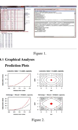
Figure 1.

4.1 _{Graphical Analyses}

Prediction Plots

Figure 2.

Variance Function (varfcn) Plots for Design Prop-erties Check:

The helpful tool in ‘rsm’ R-package is the varfcn function, which helps to see the variance of the predictions we will obtain making use of scaled variance defined by N_δ2Var[yˆ(x)]and yˆ(x)is the

pre-dicted value at the design point x . The varfcn function can also help to verify if any two of the cube blocks plus the axis block is sufficient to es-timate a second-order response surface. The y-axis is the scaled prediction variance and the x-axis measured as distance from the centre. For details see Response-surface illustration,[20].

(11)

4.2 _{EDA Plots for Cassava Plantation}

Experimental Data.

Figure 3.

The exploratory data analysis(EDA) of our da-taset in fig 3 suggest a nonlinear function as the relationship describing the plant-yield phenome-non, having fertilizer(fert) and crop spac-ing(spacing) as the explanatory variables.

Table1

4.3 _{Discussion Of Results}

Model Adequacy

The underlying assumptions of normality, inde-pendent, constant variance and homogeneity of the model error were used to verify the adequacy of our function used to describe the dataset.

The QQ-plot shows a good agreement between the distribution of the model residual and that of the standard normal distribution. This shows the adequacy and fitness of the model to the data; see-ing the pattern is linear and the points fallsee-ing within straight line of the plot i.e. points are clos-er to the straight line (See appendix I). The plot does not suggest any serious departure from our model assumptions of normality. The plot of the residual against the predictors, appendix II, show a non-systematic or random pattern in the model residual plots, therefore variance homogeneity assumption is intact. The various plots as pre-sented in the appendix gave a basis to submit that error variance of our function is normal, inde-pendent, constant and there is consistency of vari-ance of error term.

(12)

square error unchanged, a global minimum esti-mates were achieved, see appendix VI.

5 CONCLUSION

The computer intensive method-bootstrap re sam-pling method gives an access over many statisti-cal barriers involving fewer observation or sample size, such as demonstrated in this work. It has helped us in this work to evaluate the precision of the obtained estimates and we can confidently present the model with reliable estimates that re-late the non-linear relationship between cassava yields to various amount of fertilizer applied and crop spacing. The accompanied model is adequate and sufficient for the non-linear response surface.

5.1 _Appendices

Appendix III

REFERENCES

[1.]Andre I Khuri and Siuli Mukhopodhgay.

(13)

[2.]Andrew P. Robinson and Jeff D. Hamann.

Forest Analytics with An Introduction Paker PK02

[3.] Bello O.A. (2014). “Modeling Cassava Yield:

A Response Surface Methodology Ap-proach.”, Unpublished M.Sc Thesis, Universi-ty of Ibadan Nigeria, 2014.

[4.]Bello O.A. (2014).” Modeling Cassava Yield:

Response Surface Approach”, International

Journal on Computational Sciences & Appli-cations (IJCSA) Vol.4, No.3, June 2014,pg 61-70

[5.]Brian D. Ripley Professor of Applied

Statis-tics University of Oxford: How Computing has Changed Statistics (and is Changing ) [email protected]

http://www.stats.ox.ac.uk/ripley

[6.] Daniel Borcard, Francois Gillet and Pierre

Legendre. Numeric Ecology with R. Use R!

Series:ISBN 978-1-4419-7975-9

[7.]DOI 10.1007/978-1-4419-7976-6 Springer

New York Dordrecht London Heidelberg , LLC 2011

[8.] Holger Dette and Christine Kiss (2007).

“Op-timal Experimental Designs for Inverse Quad-ratic Regression Models"; Ruhr-University Bochum

[9.]Introduction to SAS,

http://help.unc.edu/statistical/applications/sas/ introsasprog.html.

[10.] J. A. Nelder(1966). “Weight Regression

Quantal Response Data, and Inverse

Polyno-mials”, The National vegetable Research

Sta-tion, Wellesbourne, Warwick, England.

[11.] J. A. Nelder(1968). “Inverse Polynomials,

A useful Group of Multi-Factor Response

Functions”; The National vegetable Research

Station, Wellesbourne, Warwick, England

[12.] Julian J. Faraway (2002). Practical

Re-gression and Anova using R. July 2002

[13.] Khuri, AI, Cornell, JA. Response

Surfac-es. 2nd edition.New York: Dekker; 1996.

[14.] Michael H. Kutner , Christopher J.

Nachtsheim , William li ;Applied Linear

Sta-tistical Models Fifth Edition ,EmORY Uni-versity UniUni-versity of Minnesota John Neter University of Georgia University of Minneso-ta

[15.] Nancy Barker. “A Practical Introduction

to The Bootstrap using SAS System”, Oxford Pharmaceutical Science, Wallingford. UK

[16.] Nduka, E.C. and T.A. Bamiduro, (1997).

“A new generalized inverse polynomial for

re-sponse surface designs”. J. Nig. Stat.

Associa-tion., 11: 41-48.

[17.] Nduka, E. C. (1994). “Inverse

polynomi-als in the Exploration of Response Surfaces”, Unpublished A Phd Thesis, U. I

(14)

Analyzing Environmental Data John Wiley $\&$ Sons, Ltd ISBN: 0-470-84836-7 (HB) page 40-46

[19.] R- CRAN:

http://cran.r-project.org/web/packages/nlrwr/index.html

[20.] Russell V. Lenth(2012).

“Response-surface illustration”, (The University of Io-wa). December 14, 2012

[21.] Schabenberger, O., Pierce, F. J., 2002.

“Contemporary statistical models for the plant and soil sciences”. CRC Press, Boca Raton, FL.

[22.] Schabenberger Oliver,"Nonlinear

Regres-sion in SAS" University of California.http:

www.ats.ucla.edu/stat/mult_pkg/faq/general/ci tingats.htm

[23.] Scholz F.W. “The Bootsrap Small Sample

Properties”. University of Washinton. Edited Staistics and Computating Series Editors: J Chamber D. Hand and W. Hardle. June 25, 2007

[24.] Tukey, J., 1962. “The future of data

anal-ysis”. Annals of Mathematical Statistics 33, 1–

67.

[25.] Whitcomb and Anderson Excerpted from

manuscript for Chapter 10 of RSM

Simpli-fied, See