Quasi-Interpolation Operators for Bivariate Quintic
Spline Spaces and Their Applications
Rengui Yu1,*, Chungang Zhu2, Xianmin Hou1and Li Yin1
1 College of Information and Management Science, Henan Agricultural University, Zhengzhou 450000, China; houxianmin83@126.com (X.H.); yinli7655@163.com (L.Y.)
2 School of Mathematical Sciences, Dalian University of Technology, Dalian 116024, China; cgzhu@dlut.edu.cn
* Correspondence: yurengui2005@163.com; Tel.: +86-371-5699-0030
Abstract:Splines and quasi-interpolation operators are important both in approximation theory and applications. In this paper, we construct a family of quasi-interpolation operators for the bivariate quintic spline spaces S3
5(∆ (2)
mn). Moreover, the properties of the proposed quasi-interpolation
operators are studied, as well as its applications for solving two-dimensional Burgers’ equation and image reconstruction. Some numerical examples show that these methods, which are easy to implement, provide accurate results.
Keywords: bivariate spline space; quasi-interpolation operator; type-2 triangulation 3; burgers’ equations; image reconstruction
1. Introduction
Spline functions are very important in both approximation theory and applications in science and engineering. Essentially, a spline is a piecewise polynomial function with certain smoothness. The special importance of spline functions is due to the mechanical meaning of univariate spline which was discussed in the famous paper written by Schoenberg [1]. Univariate splines were introduced and analyzed in the seminal paper by Schoenberg [1], although some results were obtained in the twenties (see [1], for instance). Multivariate splines are the generalizations of univariate splines. In 1976, de Boor [2] generalized univariate B-splines to multivariate splines. However, the generalizations of these kinds of definitions are inconvenient to the basic theoretical research. The study of multivariate B-splines was not active until the generalized functional expressions came up. The generalized functional expressions ( including simplex splines, Box splines and conical splines, etc. ) were given by Micchelli, de Boor-De Vore and Dahmen, et al respectively [3,4]. In 1975, Wang [5] established the so-called “smoothing cofactor-conformality method” to study the general theory on multivariate splines for any partition by using the methods of function theory and algebraic geometry. Splines have been widely applied to the fields such as function approximation, numerical analysis, Computer Geometry, Computer Aided Geometric Design, Image Processing, and so on [6–9,12,20,21]. In fact, spline functions have become a fundamental tool in these fields. Bivariate and trivariate splines are easy to store, evaluate and manipulate on a computer, so they are well suited to address the resolution of many problems of practical interest.
The paper is organized as follows. In Section 2, we study the bivariate quintic spline spaces
S35(∆(mn2)) by using the smoothing cofactor-conformality method. A family of quasi-interpolation
operators are also presented in Section 2. In Section 3, we give some examples for solving 2D Burgers’ equation and image reconstruction. Moreover, comparisons with other techniques are also provided.
2. The bivariate spline spaceS35(∆(mn2))
2.1. The spaces S3 5(∆
(2) mn)
Let D be a domain in R2, and Pk be the collection of all bivariate polynomials with real
coefficients and total degree≤k,
Pk:={p(x,y) = k
∑
i=0 k−i
∑
j=0
cijxiyj|cij∈R}. (1)
Using a finite number of irreducible algebraic curves to carry out the partition ∆, we divide the domain Dinto a finite number of sub-domains D1,D2,· · ·,DN. Each sub-domain is called a cell.
The line segments that form the boundary of each cell are called the “edges”, and intersection points of the edges are called the “vertices”. The space of multivariate spline functions is defined by
Skµ(∆):={s∈Cµ(D)|s|
Di ∈Pk,i=1,· · ·,N}. (2)
A splinesis a piecewise polynomial function of degreekpossessing continuous partial derivatives up to the orderµinD.
SupposeD= [0,m]×[0,n]for given positive integersmandn, endowed with the decomposition induced by the four-directional mesh∆(mn2)with grid lines:
x−i=0, y−i=0, x−y−i=0, x+y−i=0, i∈Z.
We have the following result [11,12].
Theorem 1. For the bivariate spline space Sµk(∆(mn2))it holds
dim Skµ(∆(mn2)) =
k+2 2
+ (3m+3n−4)
k−µ+1
2
+mn
k−2µ
2
+ (m−1)(n−1)·dµk(4), (3)
where
dµk(4):= 12k−µ−
hµ+1
3
i
+·
3k−5µ+3
hµ+1
3
i
+1.
Since each interior grid point inDis the intersection of exactly four lines from the grid partition ∆(2)
mn, the degreekand the smoothnessµmust satisfy the relationship [12]
µ< 3k−1
4 .
It is easy to see that the spacesS1 2(∆
(2) mn),S42(∆
(2) mn),S35(∆
(2)
mn)· · · have locally supported basis [12].
For S12(∆(mn2)) and S24(∆(mn2)), we refer to [12–17] for more details. We discuss the spline spaces S3
5(∆ (2)
2.2. Basis of S35(∆(mn2))
By (3), we get the dimension ofS35(∆(mn2))as follows:
dimS35(∆(mn2)) =
5+2 2
+ (3m+3n−4)
5−3+1 2
+0+ (m−1)(n−1)·4 =2mn+7m+7n+11.
(4)
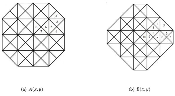
By using the smoothing cofactor-conformality method [5,12], we obtain two bivariate splines A and B whose supports are shown in Fig.1(a) and Fig.1(b). The centers of the supports are(−1/2·
h,−1/2·h) and (0, 0), respectively. Here the considered domain D is [0,mh]×[0,nh]. The local supports ofA(x,y)andB(x,y)are minimal, and forA(x,y), there are four symmetry axes:
x+1/2·h=0, y+1/2·h=0, x−y=0, x+y+h=0, while forB(x,y), there also exist four symmetry axes:
x=0, y=0, x−y=0, x+y=0. The restrictionpiof A to the cellDi(i=1,· · ·, 7), in Fig.1(a) are as follows:
p1(x,y) = 1 20h5(x−
3 2h)
4(x−5y+h),
p2(x,y) =p1(x,y) + 1
16h5(−x−y+2h)(x−y−h) 4,
p3(x,y) = 1
80h5(−x−y+2h) 5,
p5(x,y) =p2(x,y) + 1
40h5(3x−2y− 11
2 h)(x+y−h) 4,
p4(x,y) =p5(x,y) + 1
16h5(x+y−2h)(x−y−h) 4,
p6(x,y) =p5(x,y) + 1
20h5(−3x−5y−h)(x− 1 2h)
4,
p7(x,y) =p6(x,y) + 1
The restrictionqiof B to the cellDi(i=1,· · ·, 10), in Fig.1(b) are as follows:
q1(x,y) = 1
40h5(−x+ 5 2h)
5,
q2(x,y) =q1(x,y) + 1
320h5(4x+6y−13h)(x−y−2h) 4,
q3(x,y) = 1
320h5(−4x+6y+7h)(x+y−3h) 4,
q4(x,y) =q3(x,y) + 1
40h5(x+5y−9h)(x− 3 2h)
4,
q5(x,y) =q4(x,y)− 1
160h5(x+y+3h)(x+y−2h) 4,
q6(x,y) =q2(x,y) + 1
320h5(4x−6y−13h)(x+y−2h) 4,
q7(x,y) =q6(x,y) + 1
80h5(2x−13h)(x− 3 2h)
4,
q8(x,y) =q5(x,y)− 1
40h5(5x+y−13h)(y− 1 2h)
4,
q9(x,y) =q8(x,y) + 1
320h5(−6x+4y+11h)(x+y−h) 4,
q10(x,y) =q9(x,y) + 1 4h4(x−
1 2h)
4.
The expressions of the restrictions of A and B to the other cells are obtained by symmetry.
(a)A(x,y) (b)B(x,y)
Figure 1.The supports of two B-splines inS35(∆(mn2)).
Denote byAi,j,Bi,jthe translates of A and B, i.e. for all i,j∈Z
Ai,j(x,y):=A(x−ih−1
2h,y−jh− 1 2·h),
Bi,j(x,y):=B(x−ih−1
2h,y−jh− 1 2h).
(5)
It is clear that the index sets for which the functionsAi,jandBi,jdo not vanish identically onDare E={(i,j) = (α,β):−1≤α≤m+1,−1≤β≤n+1}
F={(i,j) = (α,β):−2≤α≤m+1,−2≤β≤n+1,
Since the number of these splines is 2mn+7m+7n+21, which is larger than the dimension of
S35(∆(mn2)), these splines are linearly dependent. For constructing a basis ofS53(∆ (2)
mn), we need to delete
ten splines from the ones. We have the following result.
Theorem 2. Let
G1s,t:={As,t:(s,t)∈ E\{(m−1,n),(m,n),(m+1,n),(m−1,n+1),(m,n+1)}}, G2s,t:={Bs,t:(s,t)∈F\{(m−1,n−1),(m,n−1),(m+1,n−1),(m,n),(m+1,n)}}.
Then, G1s,tS
G2s,tis a basis of S35(∆(mn2)).
Since the cardinality ofGs1,tS
Gs2,tis the same as the dimension ofS35(∆(mn2)), it is sufficient to prove
thatG1s,tS
G2s,tis a linearly independent set onD. This can be done by following the proof of Theorem 3.1 in paper [10].
By checking the sums of the appropriate Bézier coefficients, we have the following identities:
∑
(i,j)∈E
(−1)i+jAi,j(x,y) =0,
∑
(i,j)∈F(−1)i+jBi,j(x,y) =0,
∑
(i,j)∈E
Ai,j(x,y) =1,
∑
(i,j)∈FBi,j(x,y) =1.
2.3. Quasi-interpolation operators for S35(∆(mn2))
From the basis functions in the previous section, we can construct various kinds of quasi-interpolation operators.
Theorem 3. Let
L(f):=
∑
i,j∈E
f(ih−1
2h,jh− 1 2h)Ai,j,
V(f):=
∑
i,j∈F
g(ih,jh)Bi,j.
Then, for p∈P1S{xy}it holds
L(p) =p,V(p) =p,(x,y)∈D.
In applications a linear combinationCi,jof splinesAi,jandBi,jis used [18,19]. It is given by
Ci,j= 1
12(Ai,j+Ai,j+1+Ai+1,j+Ai+1,j+1) + 2 3Bi,j.
The support ofCi,j is the union of the involved splines Ak,l and Bk,l. The center of the support is
(i+1/2·h,j+1/2·h)and the number ofCi,j do not vanish identically onDismn+4m+4n+16,
which less than the dimension ofS35(∆(mn2)), so allCi,jcan only span a proper subspace ofS35(∆ (2) mn). The
shape of oneCi,jis shown in Fig.2(b). The shapes of the splines AandBare displayed in Fig.3. The
splines{Ci,j}form a partition of unity.
It is worthwhile to note that only usingCi,jwe can construct higher precision quasi-interpolation
operators by the following theorems.
LetΩ denote an open set containing Dand fi,j = f(ih,jh). Define the variation diminishing
operatorW:C(Ω)→S35(∆(mn2)):
W(f) =
m+1
∑
i=−2 n+1
∑
j=−2
fi,jCi,j. (6)
(a)Ci,j(x,y) (b)C−1,−1(x,y)
Figure 2.The support and shape ofCi,j(x,y)inS53(∆
(2)
mn).
(a) A(x,y) (b)B(x,y)
Figure 3.The shapes of two B-splines inS35(∆(mn2)).
Theorem 4. For all(x,y)∈ D, f ∈P1S
span{xy}, we have W(f)≡ f.
In order to preserve identities for all polynomials inP2andP3, we define another kinds of linear operatorsW0 :C(Ω)→S35(∆(mn2)):
W0(f) =
m+1
∑
i=−2 n+1
∑
j=−2
λi,j(f)Ci,j, (7)
where
λi,j(f) =w1· fi−1
2,j+12 +w2· fi,j+12 +w3· fi+12,j+12 +w4· fi−12,j+w5·fi,j+w6·fi+12,j+w7· fi−12,j−12 +w8·fi,j−1
2 +w9· fi+12,j−12
Note that each linear functionalλi,jdepends on nine function values of f at the grid points and the
Theorem 5. For all(x,y)∈ D, f ∈P3Sspan{x3y,xy3},
w1=w3=w7=w9=− 5 12−
1
2w8, w2=w4=w6=w8, w5= 8 3−2w8,
we have
W0(f)≡ f.
There is a unique value ofw8for which the corresponding operator is exact onP4\{x4,y4}. Theorem 6. For all(x,y)∈ D, f ∈P4\span{x4,y4},
w1=w3=w7=w9= 133
180, w2=w4=w6=w8=− 104
45 , w5= 328
45,
we have
W0(f)≡ f.
Note that Theorem6has a better result than Theorem5but at the cost of using the whole nine function values. While the conclusion of Theorem5 can be used with flexibility, i.e., having the opportunity of choosing approximatewi for given problems. The commonly used coefficientswi of
Theorem5are as follows:
w1=w3=w7=w9=− 5
12, w2=w4=w6=w8=0, w5= 8 3.
We have the following result:
Theorem 7. For all(x,y)∈ D, f ∈P3S
span{x3y,xy3}, we have W0(f)≡ f.
where
λi,j(f) =
8 3fi,j−
5 12
h
fi−1
2,j−12 +fi+12,j−12 +fi−12,j+12 +fi+12,j+12
i
To prove Theorems5-7, we need to testify the conclusions at each sub-regionDij = [xi,xi+1]× [yj,yj+1](see Fig.4(a)). For I in Dij, we have a properly posed set of nodes for multivariate spline
interpolation (21 points, see Fig.4(b)) [12]. Next, by computing the values of(W0f)(x,y) in (7) at these 21 points( noted byP), we get the fact that(W0f)(p) = f(p),∀p ∈ P. The same fact can be
obtained similarly forI I,I I I,IVinDij, respectively. Hence, these theorems hold by the arbitrariness
ofDij.
In the next section, we give two applications of the quasi-interpolation operatorW0in Theorem
7.
3. Applications of quasi-interpolation operatorW0
3.1. Solving 2D Burgers’ equations
Here we consider the system of 2D Burgers’ equations [32]. One can refer to [32,33] for more details.
ut+uux+vuy= 1
R(uxx+uyy), vt+uvx+vvy= 1
R(vxx+vyy),
(a)Dij (b) Properly posed set of nodes for interpolation.
Figure 4.Sub-region ofD.
with initial conditions
u(x,y, 0) = f(x,y), (x,y)∈D,
v(x,y, 0) =g(x,y), (x,y)∈D, (9)
and boundary conditions:
u(x,y,t) = f1(x,y,t), (x,y)∈∂D, t>0, v(x,y,t) =g1(x,y,t), (x,y)∈∂D, t>0,
(10)
whereD = {(x,y) | a ≤ x ≤ b,a ≤ y ≤ b}and∂Ddenotes its boundary. Functionsu andv are the velocity components to be determined,f,g,f1andg1are known functions, andRis the Reynolds number.
Discretizing Burgers’ equations (8) in the time domain with step τ and using the derivatives
of (W0u)(x,y),(W0v)(x,y) defined in Theorem 7 to approximate the corresponding derivatives of
u(x,y,t)andv(x,y,t)yields
uni,+j 1=uin,j+τ(1 R(((W
0u)
xx)ni,j+ ((W0u)yy)ni,j)−unij((W0u)x)ni,j−vni,j((W0u)y)ni,j), vni,+j 1=vni,j+τ(1
R(((W
0v)
xx)ni,j+ ((W0v)yy)ni,j)−unij((W0v)x)ni,j−vni,j((W0v)y)ni,j),
(11)
where uni,j,vni,j are the approximation of the value of u(x,y,t),v(x,y,t) at the uniform mesh grid (ihx,jhy,tτ). This scheme provides a numerical solution for Burgers’ equation, which is called
multivariate spline quasi-interpolation (abbr. MSQI) scheme.
By iterating this scheme, we obtain the numerical solution for Burgers’ equations. We give the following examples.
Example 1A Hopf-Cole transformation [34] allows to determine the exact solution
u(x,y,t) =3 4 −
1
4(1+e(R(−t−4x+4y))/32), u(x,y,t) =3
4 +
1
4(1+e(R(−t−4x+4y))/32),
(12)
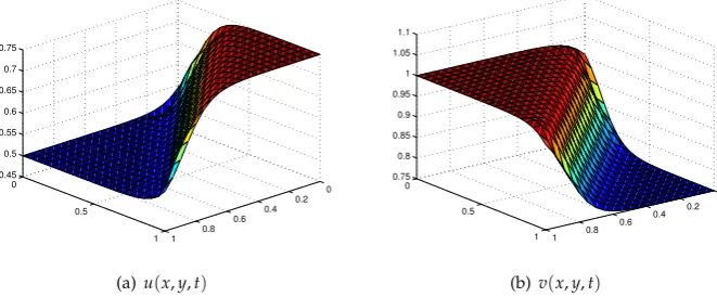
computational domain D = {(x,y) : 0 ≤ x ≤ 1, 0 ≤ y ≤ 1}. For the uniform mesh grid we use a looser ones withhx=hy=0.1 for a lower computation.
0 0.2 0.4 0.6 0.8 1 0
0.5
1 0.45
0.5 0.55 0.6 0.65 0.7 0.75
(a)u(x,y,t)
0 0.2 0.4 0.6 0.8 1 0
0.5
1 0.75
0.8 0.85 0.9 0.95 1 1.05 1.1
(b)v(x,y,t)
Figure 5. A numerical illustration of approximation solutionsu(x,y,t)(a) andv(x,y,t)(b) by MSQI withR=80,τ=10−4,hx=hy=0.1 att=0.5.
Figs.5(a) and 5(b)show the approximation solutions of u(x,y,t) and v(x,y,t) at steady state respectively. In the meanwhile, the numerical solution for different times and different mesh grid points are given in Tables1and2.
Table 1.Comparison of the numerical results by MSQI with exact solutionsu(x,y,t)withR=80,τ= 10−4at different timet.
Mesh grid t=0.05 t=0.2 t=0.5
unum uexact unum uexact unum uexact
(0.1,0.1) 0.61749 0.61720 0.59474 0.59439 0.55564 0.55568
(0.9,0.2) 0.50021 0.50020 0.50015 0.50014 0.50006 0.50007
(0.8,0.3) 0.50150 0.50148 0.50108 0.50102 0.50049 0.50048
(0.9,0.5) 0.50403 0.50398 0.50289 0.50275 0.50155 0.50130
(0.8,0.6) 0.52640 0.52667 0.51859 0.51896 0.50990 0.50933
(0.2,0.8) 0.74931 0.74930 0.74900 0.74898 0.74783 0.74786
(0.9,0.9) 0.61720 0.61720 0.59456 0.59439 0.55369 0.55568
Table 2.Comparison of the numerical results by MSQI with exact solutionsv(x,y,t)withR=80,τ= 10−4at different timet.
Mesh grid t=0.05 t=0.2 t=0.5
vnum vexact vnum vexact vnum vexact
(0.1,0.1) 0.88251 0.88280 0.90526 0.90561 0.94436 0.94432
(0.9,0.2) 0.99979 0.99980 0.99985 0.99986 0.99994 0.99993
(0.8,0.3) 0.99850 0.99852 0.99892 0.99898 0.99951 0.99952
(0.9,0.5) 0.99597 0.99602 0.99711 0.99725 0.99845 0.99869
(0.8,0.6) 0.97360 0.97333 0.98141 0.98104 0.99010 0.99067
(0.2,0.8) 0.75069 0.75070 0.75100 0.75102 0.75217 0.75214
(0.9,0.9) 0.88250 0.88280 0.90544 0.90561 0.94632 0.94432
Table 3.Comparison of absolute errors foru(x,y,t)withR=80,τ=10−4at different timet.
Mesh grid t=0.01 t=0.5
MSQI Bahadir[32] Zhu[35] MSQI Bahadir[32] Zhu[35]
(0.1,0.1) 1.63803E-5 7.24132E-5 5.91368E-5 6.11973E-4 5.13431E-4 2.77664E-4
(0.5,0.1) 1.85815E-5 2.42869E-5 4.84030E-6 1.73489E-4 8.85712E-4 4.52081E-4
(0.9,0.1) 1.64831E-7 8.39751E-6 3.41000E-8 3.07314E-6 6.53372E-5 3.37430E-6
(0.3,0.3) 1.65880E-5 8.25331E-5 5.91368E-5 6.69829E-4 7.31601E-4 2.77664E-4
(0.7,0.3) 1.94033E-5 3.43163E-5 4.84030E-6 2.16464E-4 6.27245E-4 4.52081E-4
(0.1,0.5) 1.61309E-7 5.62014E-5 1.64290E-6 3.32546E-4 4.01942E-4 2.86553E-4
Table 4.Comparison of absolute errors forv(x,y,t)withR=80,τ=10−4at different timet.
Mesh grid t=0.01 t=0.5
MSQI Bahadir[32] Zhu[35] MSQI Bahadir[32] Zhu[35]
(0.1,0.1) 1.63803E-5 8.35601E-5 5.91368E-5 6.11973E-4 6.17325E-4 2.77664E-4
(0.5,0.1) 1.85815E-5 5.13642E-5 4.84030E-6 1.73489E-4 4.67046E-4 4.52081E-4
(0.9,0.1) 1.64832E-7 7.03298E-6 3.41000E-8 3.07314E-6 1.70434E-5 3.37400E-6
(0.3,0.3) 1.65880E-5 6.15201E-5 5.91368E-5 6.69829E-4 6.25402E-4 2.77664E-4
(0.7,0.3) 1.94033E-5 5.41000E-5 4.84030E-6 2.16464E-4 4.66046E-4 4.52081E-4
(0.1,0.5) 1.61310E-7 7.35192E-5 1.64290E-6 3.32546E-4 8.72422E-4 2.86553E-4
Example 2In the second problem, we consider the 2D Burgers’ equations with the following initial conditions [33]
u(x,y, 0) =x+y,
v(x,y, 0) =x−y,
and the computational domain has been taken asD={(x,y): 0≤x ≤0.5, 0≤ y≤0.5}. The exact solutions are as follows:
u(x,y,t) = x+y−2xt 1−2t2 , v(x,y,t) = x−y−2yt
1−2t2 .
Numerical results using MSQI method are listed in Tables5and6. In these two tables we also provide numerical errors and comparison with those given in [35]. All the results in Tables5and6are calculated with uniform mesh gridhx = hy = 0.05, time step sizeτ =10−4and arbitrary Reynolds
numberRat different timet. In Figs.6(a)and6(b), we have plotted the profiles of the approximation solutions by MSQI method att=0.1.
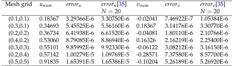
Table 5.Comparison of numerical solutions with the exact solutions foruandvatt=0.1,N =10, and errors are absolute errors.
Mesh grid unum erroru erroru[35] vnum errorv errorv[35]
N=20 N=20
(0.1,0.1) 0.18367 3.29366E-6 3.30750E-6 -0.02041 7.46922E-7 1.05384E-6
(0.3,0.1) 0.34693 5.45525E-6 5.56160E-6 0.18367 3.14176E-6 3.30770E-6
(0.2,0.2) 0.36734 6.41938E-6 6.61520E-6 -0.04081 1.80110E-6 2.10766E-6
(0.4,0.2) 0.53060 8.79085E-6 8.86940E-6 0.16326 2.16219E-6 2.25400E-6
Table 6.Comparison of numerical solutions with the exact solutions foruandvatt=0.4,N =10, and errors are absolute errors.
Mesh grid unum erroru erroru[35] vnum errorv errorv[35]
N=20 N=20
(0.1,0.1) 0.17645 1.56636E-5 1.01945E-4 -0.11762 2.30003E-5 3.54833E-4
(0.3,0.1) 0.23529 4.91795E-6 5.58724E-4 0.17646 1.53797E-5 1.01946E-4
(0.2,0.2) 0.35291 3.32840E-5 2.03891E-4 -0.23524 5.73342E-5 7.09666E-4
(0.4,0.2) 0.41174 2.52872E-5 6.60670E-4 0.05884 1.73085E-5 4.56779E-4
(0.3,0.3) 0.52936 5.66418E-5 3.05837E-4 -0.35284 1.04665E-4 1.06450E-3 (0.2,0.4) 0.64701 5.11863E-5 4.89963E-4 -0.76460 1.07043E-4 1.67222E-3 (0.5,0.5) 0.88225 1.03951E-4 5.09728E-4 -0.58804 1.92169E-4 1.77417E-3
0 0.1 0.2 0.3 0.4 0.5 0
0.1 0.2
0.3 0.4
0.5 0
0.5 1
(a)u(x,y,t)
0 0.1 0.2 0.3 0.4 0.5 0
0.1 0.2
0.3 0.4
0.5 −1
−0.5 0 0.5 1
(b)v(x,y,t)
From these tables we can see that MSQI scheme achieves an excellent approximation with the exact solutions of the equations. Though some of the results are not better than the ones in [35], MSQI method has a simpler construction, easy implementation, lower time consuming and smaller calculation.
3.2. Image reconstruction
Digital-image-processing technique is applied more and more extensively at present, which can be seen in real-time image transmission, digital image restoration, extracting facial features, image synthesis, image compression and encryption, and so on [36,37].
In this section, we use the multivariate spline quasi-interpolation operator W0 defined by Theorem7 to deal with problems of image reconstruction. For the testing image, we use 2D gray imageLena[31] with pixels of 256×256, which can be seen in Fig.7(a).
(a) original (b) sampling pixels (c) byW0f inS3 5(∆
(2) mn)
Figure 7.Results of 2D gray imageLena.
Fig.7(b) is the 32768 (256 ×128) sampling pixels from Lena which are used in the quasi-interpolation operatorW0. The reconstruction image ofLenais shown in Fig.7(c). Also we give the reconstruction image ofLenaby using the quasi-interpolation operatorWmn[11,12] inS12(∆(mn2))in
Fig.8(c). For the operatorWmn, we can see [11,12] for more details. Drawings of partial enlargement
of the reconstruction images withW0andWmnare illustrated in Fig.8(a)and8(b)respectively.
(a) partial enlarged inS3 5(∆
(2)
mn) (b) partial enlarged inS12(∆ (2)
mn) (c) byWmninS12(∆ (2) mn)
Figure 8. Reconstructed image byWmn (c) and partial enlarged image of reconstructions byW0 (a) andWmn(b).
We also have usedBarbaraandPeppers2D gray images to test the performance of the operator
(a) original (b) sampling pixels (c) byW0inS3 5(∆
(2) mn)
Figure 9.Results of 2D gray imageBarbara.
(a) original (b) sampling pixels (c) byW0inS3 5(∆
(2) mn)
Figure 10.Results of 2D gray imagePeppers.
become bigger in contrast with the original ones. Note that the operatorW0 can also serve as one technique for problems with image zooming in and out. Other quasi-interpolation operators can also be used for these problems.
Acknowledgments: This work is partly supported by the National Natural Science Foundation of China (Nos. 11671068, 11271060) and the Fundamental Research Funds for the Central Universities (Nos. DUT16LK38).
Author Contributions:Rengui Yu, Chungang Zhu designed the research. Rengui Yu, Xianmin Hou, Li Yin were responsible for all simulations and analyses of the results. Rengui Yu wrote the paper.
Conflicts of Interest:The authors declare no conflict of interest.
References
1. I J. Schoenberg. Contributions to the problem of approximation of equidistant data by analytic functions.
Quart. Appl. Math.1946,4(1/2), 45-99,112-141.
2. C. de Boor. Splines as linear comination of B-splines, in "Approximation Theory II", G.G.Lorentz, C.K. Chui and L.L.Schumaker(eds.), Acad. Press, New York, 1976, 1-47.
3. C. de Boor. Topics in multivariate approximation theory, in "Topics in Numerical Analysis", P.R. Turner (ed.), Lecture Notes Mathematics, Springer-Verlag, 965(1982),39-78.
4. W. Dahmen; C.A. Micchelli. Recent prograss in multivariate splines, interpolating cardinal splines as their degree rends to infinity, Israel J.Ward (eds.), Academic press, 1983, 27-121.
5. R.H. Wang. The structural characterization and interpolation for multivariate splines. Acta Math. Sinica
1975,18, 91-106.
6. C. de Boor.A Practical Guide to Splines; Springer, NewYork, USA, 1978.
7. C. Allouch; P. Sablonnière; D. Sbibih. A collocation method for the numerical solution of a two dimensional integral equation using a quadratic spline quasi-interpolant.Numerical algorithms2013,62(3), 445-468. 8. C. Dagnino; S. Remogna; P. Sablonnière. On the solution of Fredholm integral equations based on spline
9. C. Dagnino; P. Lamberti; S. Remogna. Curve network interpolation by C1 quadratic B-spline surfaces.
Computer Aided Geometric Design2015,40, 26-39.
10. C.K. Chui; R.H. Wang. Spaces of bivariate cubic and quartic splines on type-1 triangulation.J. Math. Anal. Appl.1984,101, 540-554.
11. R.H. Wang. The dimension and basis of spaces of multivariate splines.Jour. Comput. Appl. Math.1985,12-13, 163-177.
12. R.H. Wang.Multivariate Spline Functions and Their Applications; Science Press/Kluwer Academic Publishers: Beijing/New York/Dordrecht/Boston/London, 2001.
13. R.H. Wang; C.J. Li. Bivariate quartic spline spaces and quasi-interpolation operators. Jour. Comp. Appl. Math.2006,190, 325-338.
14. F. Foucher; P. Sablonnière. Approximating partial derivatives of first and second order by quadratic spline quasi-interpolants on uniform meshes.Math. Comput. Simulation2008,77, 202-208.
15. C. Dagnino; P. Lamberti. On the construction of local quadratic spline quasi-interpolants on bounded rectangular domains.J. Comp. Appl. Math.2008,221(2), 367-375.
16. C. Dagnino; P. Lamberti; S. Remogna. B-spline bases for unequally smooth quadratic spline spaces on non-uniform criss-cross triangulations.Numerical algorithms2012,61(2), 209-222.
17. C. Dagnino; S. Remogna; P. Sablonnière. Error bounds on the approximation of functions and partial derivatives by quadratic spline quasi-interpolants on non-uniform criss-cross triangulations of a rectangular domain.BIT Numerical Mathematics2013,53(1), 87-109.
18. C.J. Li. Multivariate Splines on Special Triangulations and Their Applications, PhD thesis, Department of Applied Mathematics, Dalian University of Technology, 2004.
19. M.W. Song. Piecewise quintic spline spaces on uniform type-2 triangulation, School of Mathematical Sciences, Dalian University of Technology, 2007.
20. C.G. Zhu; R.H. Wang. Lagrange interpolation by bivariate splines on cross-cut partitions.Jour. Comp. Appl. Math.2006,195, 326-340.
21. C.G. Zhu; R.H. Wang. Numerical solution of Burgers’ equation by cubic B-spline quasi-interpolation.Appl. Math. Comput.2009,208, 260-272.
22. M. Basto; V. Semiao; F. Calheiros. Dynamics and synchronization of numerical solutions of the Burgers equation.Jour. Comp. Appl. Math.2009,231, 793-806.
23. W.M. Moslem; R. Sabry. Zakharov-Kuznetsov-Burgers equation for dust ion acoustic waves.Chaos Solitons Fractals2008,36, 628-634.
24. M.M. Rashidi; E. Erfani. New analytical method for solving Burgers’ and nonlinear heat transfer equations and comparison with HAM.Comput. Phys. Commun.2009,180, 1539-1544.
25. S. Abbasbandy; M.T. Darvishi. A numerical solution of Burgers’ equation by modified Adomian’s decomposition method.Appl. Math. Comput.2005,163, 1265-1272.
26. M. Dehghan; A. Hamidi; M. Shakourifar. The solution of coupled Burgers’ equation using Adomian-Pade technique.Appl. Math. Comput.2007,189, 1034-1047.
27. S. Abbasbandy; M.T. Darvishi. A numerical solution of Burgers’ equation by time discretization of Adomian’s decomposition method.Appl. Math. Comput.2005,170, 95-102.
28. B. Zhou; Y.N. Peng; C.M. Ye; J. Tang. GPGPU Accelerated Fast Convolution Back-Projection for Radar Image Reconstruction.Tsinghua Science&Technology2011,16(3), 256-263.
29. A. Ouaddah; D. Boughaci. Harmony search algorithm for image reconstruction from projections. Applied Soft Computing2016,46, 924-935.
30. S. U ¯gur; O. Arikan. SAR image reconstruction and autofocus by compressed sensing. Digital Signal Processing2012,22(6), 923-932.
31. http://www.ece.rice.edu/ wakin/images/.
32. A.R. Bahadir. A fully implicit finite-difference scheme for two-dimensional Burgers’ equations.Appl. Math. Comput.2003,137, 131-137.
33. J. Biazar; H. Aminikhah. Exact and numerical solutions for non-linear Burgers’ equation by VIM.Math. Comput. Modelling2009,49, 1394-1400.
35. H.Q. Zhu; H.Z. Shu; M.Y. Ding. Numerical solutions of two-dimensional Burgers’ equations by discrete Adomian decomposition method.Comput. Math. Appl.2010,60, 840-848.
36. D. Chaikalis; N.P. Sgouros; D. Maroulis. A real-time FPGA architecture for 3D reconstruction from integral images.Journal of Visual Communication and Image Representation2010,21, 9-16.
37. J.Z. Huang; S.T. Zhang; D. Metaxas. Efficient MR image reconstruction for compressed MR imaging.
Medical Image Analysis2011,15, 670-679.
c