Lightweight MDS Involution Matrices (Full version)
Siang Meng Sim1, Khoongming Khoo2, Fr´ed´erique Oggier1, and Thomas Peyrin1
1
Nanyang Technological University, Singapore 2 DSO National Laboratories, Singapore
[email protected], [email protected], [email protected], [email protected]
Abstract. In this article, we provide new methods to look for lightweight MDS matrices, and in particular involutory ones. By proving many new properties and equivalence classes for various MDS matrices constructions such as circulant, Hadamard, Cauchy and Hadamard-Cauchy, we exhibit new search algorithms that greatly reduce the search space and make lightweight MDS matrices of rather high dimension possible to find. We also explain why the choice of the irreducible polynomial might have a significant impact on the lightweightness, and in contrary to the classical belief, we show that the Hamming weight has no direct impact. Even though we focused our studies on involutory MDS matrices, we also obtained results for non-involutory MDS matrices. Overall, using Hadamard or Hadamard-Cauchy constructions, we provide the (involutory or non-involutory) MDS matrices with the least possible XOR gates for the classical dimensions 4×4, 8×8, 16×16 and 32×32 in GF(24) and GF(28). Compared to the best known matrices, some of our new candidates save up to 50% on the amount of XOR gates required for an hardware implementation. Finally, our work indicates that involutory MDS matrices are really interesting building blocks for designers as they can be implemented with almost the same number of XOR gates as non-involutory MDS matrices, the latter being usually non-lightweight when the inverse matrix is required.
Key words:lightweight cryptography, Hadamard matrix, Cauchy matrix, involution, MDS.
1
Introduction
Most symmetric key primitives, like block ciphers, stream ciphers or hash functions, are usually based on various components that provide confusion and diffusion. Both concepts are very important for the overall security and efficiency of the cryptographic scheme and extensive studies have been conducted to find the best possible building blocks. The goal of diffusion is basically to spread the internal dependencies as much as possible. Several designs use a weak yet fast diffusion layer based on simple XOR, addition and shifting operation, but another trend is to rely on strong linear diffusion matrices, like Maximal Distance Separable (MDS) matrices. A typical example is the AES
cipher [17], which uses a 4×4 matrix in GF(28) to provide diffusion among a vector of 4 bytes. These mathematical objects ensure the designers a perfect diffusion (the underlying linear code meets the Singleton bound), but can be quite heavy to implement. Software performances are usually not so much impacted as memory is not really constrained and table-based implementations directly incorporate the field multiplications in the stored values. However, hardware implementations will usually suffer from an important area requirement due to the Galois field multiplications. The impact will also be visible on the efficiency of software bitslice implementations which basically mimic the hardware computations flow.
Good hardware efficiency has became a major design trend in cryptography, due to the increasing importance of ubiquitous computing. Many lightweight algorithms have recently been proposed, notably block ciphers [12, 14, 19, 9] and hash functions [4, 18, 11]. The choice of MDS matrices played an important role in the reduction of the area required to provide a certain amount of security. In PHOTON, the hash function [18] that was proposed a new type of MDS matrix that can be computed in a serial or recursive manner. This construction greatly reduces the temporary memory (and thus the hardware area) usually required for the computation of the matrix. Such matrices were later used inLED[19] block cipher, or PRIMATEs[1] authenticated encryption scheme, and were further studied and generalized in subsequent articles [30, 34, 3, 2, 10]. Even though these serial matrices provide a good way to save area, this naturally comes at the expense of an increased number of cycles to apply the matrix. In general, they are not well suited for round-based or low-latency implementations.
Another interesting property for an MDS matrix to save area is to be involutory. Indeed, in most use cases, encryption and decryption implementations are required and the inverse of the MDS matrix will have to be implemented as well (except for constructions like Feistel networks, where the inverse of the internal function is not needed for decryption). For example, the MDS matrix ofAESis quite lightweight for encryption, but not really for decryption3. More generally, it is a valuable advantage that one can use exactly the same diffusion matrix for encryption and decryption. Some ciphers like ANUBIS [5], KHAZAD [6], ICEBERG [33] or PRINCE [13] even pushed the involution idea
c
IACR 2015. This article is the full version of the preproceeding version in FSE 2015.
a bit further by defining a round function that is almost entirely composed of involution operations, and where the non-involution property of the cipher is mainly provided by the key schedule.
There are several ways to build a MDS matrix [35, 24, 27, 31, 20, 15], a common method being to use a circulant construction, like for theAESblock cipher [17] or theWHIRLPOOLhash function [8]. The obvious benefit of a circulant matrix for hardware implementations is that all of its rows are similar (up to a right shift), and one can trivially reuse the multiplication circuit to save implementation costs. However,it has been proven in [23] that circulant matrices of order 4 cannot be simultaneously MDS and involutory. And very recently Guptaet al.[21] proved that circulant MDS involutory matrices do not exist. Finding lightweight matrices that are both MDS and involutory is not an easy task and this topic has attracted attention recently. In [31], the authors consider Vandermonde or Hadamard matrices, while in [35, 20, 15] Cauchy matrices were used. Even if these constructions allow to build involutory MDS matrices for big matrix dimensions, it is difficult to find the most lightweight candidates as the search space can become really big.
Our contributions. In this article, we propose a new method to search for lightweight MDS matrices, with an important focus on involutory ones. After having recalled the formula to compute the XOR count, i.e. the amount of XORs required to evaluate one row of the matrix, we show in Section 2 that the choice of the irreducible polynomial is important and can have a significant impact on the efficiency, as remarked in [26]. In particular, we show that the best choice is not necessarily a low Hamming weight polynomial as widely believed, but instead one that has a high standard deviation regarding its XOR count. Then, in Section 3, we recall some constructions to obtain (involutory) MDS matrices: circulant, Hadamard, Cauchy and Cauchy-Hadamard. In particular, we prove new properties for some of these constructions, which will later help us to find good matrices. In Section 4 we prove the existence of equivalent classes for Hadamard matrices and involutory Hadamard-Cauchy matrices and we use these considerations to conceive improved search algorithms of lightweight (involutory) MDS matrices. We describe these new algorithms in Section 5 for lightweight involutory MDS matrices. Our methods can also be relaxed and applied to the search of lightweight non-involutory MDS matrices as explained in Section 6. These algorithms are significant because they are feasible exhaustive search while the search space of the algorithms described in [20, 15] is too big to be exhausted4. Our algorithms guarantee that the matrices found are the lightest according to our metric.
Overall, using Hadamard or Hadamard-Cauchy constructions, we provide the smallest known (involutory or non-involutory) MDS matrices for the classical dimensions 4×4, 8×8, 16×16 and 32×32 in GF(24) and GF(28). The designers of one of the CAESAR competition candidates, Joltik [22], have used one of the matrices that we have found to build their primitive. All our results are summarized and commented in Section 7. Surprisingly, it seems that involutory MDS matrices are not much more expensive than non-involutory MDS ones, the former providing the great advantage of a free inverse implementation as well. We recall that in this article we are not considering serial matrices, as their evaluation either requires many clock cycles (for serial implementations) or an important area (for round-based implementations).
Notations and preliminaries. We denote by GF(2r) the finite field with 2relements,r≥1. This field is isomorphic
to polynomials in GF(2)[X] modulo an irreducible polynomialp(X) of degreer, meaning that every field element can be seen as a polynomial α(X) with coefficients in GF(2) and of degree r−1: α(X) = Pr−1
i=0biXi, bi ∈ GF(2),
0 ≤i ≤ r−1. The polynomialα(X) can also naturally be viewed as an r-bit string (br−1, br−2, ..., b0). In the rest of the article, an element α in GF(2r) will be seen either as the polynomial α(X), or the r-bit string represented
in a hexadecimal representation, which will be prefixed with0x. For example, in GF(28), the 8-bit string 00101010 corresponds to the polynomialX5+X3+X, written0x2ain hexadecimal.
The addition operation on GF(2r) is simply defined as a bitwise XOR on the coefficients of the polynomial rep-resentation of the elements, and does not depend on the choice of the irreducible polynomial p(X). However, for multiplication, one needs to specify the irreducible polynomialp(X) of degreer. We denote this field as GF(2r)/p(X),
wherep(X) can be given in hexadecimal representation5. The multiplication of two elements is then the modulop(X) reduction of the product of the polynomial representations of the two elements.
Finally, we denote byM[i, j] the (i, j) entry of the matrixM, we start the counting from 0, that isM[0,0] is the entry corresponding to the first row and first column.
2
Analyzing XOR count according to different finite fields
In this section, we explain the XOR count that we will use as a measure to evaluate the lightweightness of a given matrix. Then, we will analyze the XOR count distribution depending on the finite field and irreducible polynomial
4
The huge search space issue can be reduced if one could search intelligently only among lightweight matrix candidates. However, this is not possible with algorithms from [20, 15] since the matrix coefficients are known only at the end of the matrix generation, and thus one cannot limit the search to lightweight candidates only.
5 This should not be confused with the explicit construction of finite fields, which is commonly denoted as GF(2r)[X]/(P),
considered. Although it is known that finite fields of the same size are isomorphic to each other and it is believed that the security of MDS matrices is not impacted by this choice, looking at the XOR count is a new aspect of finite fields that remains unexplored in cryptography.
2.1 The XOR count
It is to note that the XOR count is an easy-to-manipulate and simplified metric, but MDS coefficients have often been chosen to lower XOR count, e.g. by having low Hamming weight. As shown in [26], low XOR count is strongly correlated minimization of hardware area.
Later in this article, we will study the hardware efficiency of some diffusion matrices and we will search among huge sets of candidates. One of the goals will therefore be to minimize the area required to implement these lightweight matrices, and since they will be implemented with XOR gates (the diffusion layer is linear), we need a way to easily evaluate how many XORs will be required to implement them. We explain our method in this subsection.
In general, it is known that low Hamming weight generally requires lesser hardware resource in implementations, and this is the usual choice criteria for picking a matrix. For example, the coefficients of theAESMDS matrix are 1, 2 and 3, in a hope that this will ensure a lightweight implementation. However, it was shown in [26] that while this heuristic is true in general, it is not always the case. Due to some reduction effects, and depending on the irreducible polynomial defining the computation field, some coefficients with not-so-low Hamming weight might be implemented with very few XORs.
Definition 1 The XOR count of an elementαin the fieldGF(2r)/p(X)is the number of XORs required to implement
the multiplication ofαwith an arbitrary β overGF(2r)/p(X).
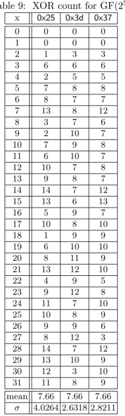
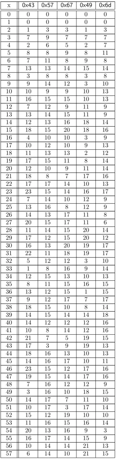
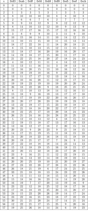
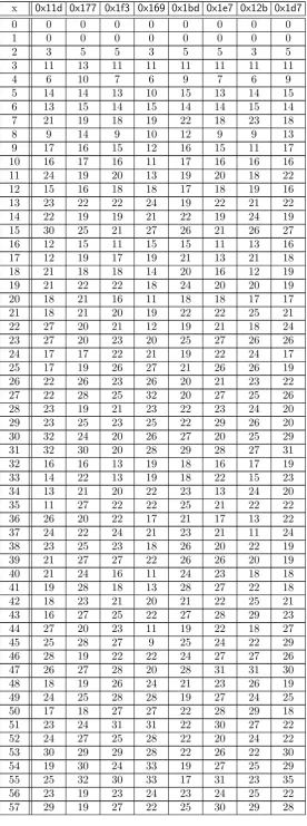
For example, let us explain how we compute the XOR count of α= 3 over GF(24)/0x13 and GF(24)/0x19. Let (b3, b2, b1, b0) be the binary representation of an arbitrary elementβ in the field. For GF(24)/0x13, we have:
(0,0,1,1)·(b3, b2, b1, b0) = (b2, b1, b0⊕b3, b3)⊕(b3, b2, b1, b0) = (b2⊕b3, b1⊕b2, b0⊕b1⊕b3, b0⊕b3), which corresponds to 5 XORs6. For GF(24)/0x19, we have:
(0,0,1,1)·(b3, b2, b1, b0) = (b2⊕b3, b1, b0, b3)⊕(b3, b2, b1, b0) = (b2, b1⊕b2, b0⊕b1, b0⊕b3),
which corresponds to 3 XORs. One can observe that XOR count is different depending on the finite field defined by the irreducible polynomial.
In order to calculate the number of XORs required to implement an entire row of a matrix, we can use the following formula given in [26]:
XOR count for one row ofM = (γ1, γ2, ..., γk) + (n−1)·r, (1)
whereγiis the XOR count of thei-th entry in the row ofM,nbeing the number of nonzero elements in the row and
rthe dimension of the finite field.
For example, the first row of theAESdiffusion matrix being (1,1,2,3) over the field GF(28)/0x11b, the XOR count for the first row is (0 + 0 + 3 + 11) + 3×8 = 38 XORs (the matrix being circulant, all rows are equivalent in terms of XOR count).
2.2 XOR count for different finite fields
We programmed a tool that computes the XOR count for every nonzero element over GF(2r) forr= 2, . . . ,8 and for
all possible irreducible polynomials are provided in Appendix D. By analyzing the outputs of this tool, we could make two observations that are important to understand how the choice of the irreducible polynomial affects the XOR count. Before presenting our observations, we state some terminologies and properties related to reciprocal polynomials in finite fields.
Definition 2 A reciprocal polynomial 1p(X)of a polynomialp(X)overGF(2r), is a polynomial expressed as 1
p(X) =
Xr·p(X−1). A reciprocal finite field, K = GF(2r)/1
p(X), is a finite field defined by the reciprocal polynomial which
definesF= GF(2r)/p(X).
In other words, a reciprocal polynomial is a polynomial with the order of the coefficients reversed. For example, the reciprocal polynomial ofp(X) =0x11bin GF(28) is p1(X) =0x11b1 =0x1b1. It is also to be noted that the reciprocal polynomial of an irreducible polynomial is also irreducible.
6 We acknowledge that one can perform the multiplication with 4 XORs as b
The total XOR count. Our first new observation is that even if for an individual element of the field the choice of the irreducible polynomial has an impact on the XOR count, the total sum of the XOR count over all elements in the field is independent of this choice. We state this in the following theorem, the proof being provided in Appendix A. Theorem 1 The total XOR count for a field GF(2r)isrPr
i=22i−2(i−1), where r≥2.
From Theorem 1, it seems that there is no clear implication that one irreducible polynomial is strictly better than another, as the mean XOR count is the same for any irreducible polynomial. However, the irreducible polynomials have different distribution of the XOR count among the field elements, that is quantified by the standard deviation. A high standard deviation implies that the distribution of XOR count is very different from the mean, thus there will be more elements with relatively lower/higher XOR count. In general, the order of the finite field is much larger than the order of the MDS matrix and since only a few elements of the field will be used in the MDS matrices, there is a better chance of finding an MDS matrix with lower XOR count.
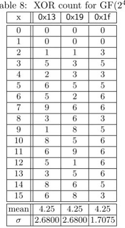
Hence, our recommendation is to choose the irreducible polynomial with the highest standard deviation regarding the XOR count distribution. From previous example, in GF(24) (XOR count mean equals 4.25 for this field dimension), the irreducible polynomials0x13and0x19lead to a standard deviation of 2.68, while0x1f leads to a standard deviation of 1.7075. Therefore, the two first polynomials seem to be a better choice. This observation will allow us to choose the best irreducible polynomial to start with during the searches. We refer to Appendix D for all the standard deviations according to the irreducible polynomial.
We note that the folklore belief was that in order to get lightweight implementations, one should use a low Hamming weight irreducible polynomial. The underlying idea is that with such a polynomial less XORs might be needed when the modular reduction has to be applied during a field multiplication. However, we have shown that this is not necessarily true. Yet, by looking at the data from Appendix D, we remark that the low Hamming weight irreducible polynomials usually have a high standard deviation, which actually validates the folklore belief. We conjecture that this heuristic will be less and less exact when we go to higher and higher order fields.
Matching XOR count. Our second new observation is that the XOR count distribution implied by a polynomial will be the same compared to the distribution of its reciprocal counterpart. We state this observation in the following theorem, the proof being provided in Appendix B.
Theorem 2 There exists an isomorphic mapping from a primitive α ∈ GF(2r)/p(X) to another primitive β ∈
GF(2r)/1
p(X)where the XOR count ofα
i andβi is equal for eachi={1,2, ...,2r−1}.
In Appendix C, we listed all the primitive mapping from a finite field to its reciprocal finite field for all fields GF(2r) with r = 2, . . . ,8 and for all possible irreducible polynomials. We give an example to illustrate our theorem. For GF(24), there are three irreducible polynomials: 0x13,0x19 and0x1f and the XOR count for the elements are shown in Appendix D. From the binary representation we see that 0x1
13 = 0x19. Consider an isomorphic mapping φ : GF(24)/0x13→GF(24)/0x19 defined asφ(2) = 12, where 2 and 12 are the primitives for the respective finite fields. Table 4 of Appendix C shows that the order of the XOR count is the same.
We remark that for a self-reciprocal irreducible polynomial, for instance 0x1f in GF(24), there also exists an automorphism mapping from a primitive to another primitive with the same order of XOR count (see Appendix C).
Theorem 2 is useful for understanding that we do not need to consider GF(2r)/1p(X) when we are searching for lightweight matrices. As there exists an isomorphic mapping preserving the order of the XOR count, any MDS matrix over GF(2r)/1
p(X) can be mapped to an MDS matrix over GF(2
r)/p(X) while preserving the XOR count. Therefore,
it is redundant to search for lightweight MDS matrices over GF(2r)/1p(X) as the lightest MDS matrix can also be found in GF(2r)/p(X). This will render our algorithms much more efficient: when using exhaustive search for low XOR count MDS over finite field defined by various irreducible polynomial, one can reduce the search space by almost a factor 2 as the reciprocal polynomials are redundant.
3
Types of MDS matrices and properties
In this section, we first recall a few properties of MDS matrices and we then explain various constructions of (involutory) MDS matrices that were used to generate lightweight candidates. Namely, we will study 4 types of diffusion matrices: circulant, Hadamard, Cauchy, and Hadamard-Cauchy. We recall that we do not consider serially computable matrices in this article, like the ones described in [18, 19, 30, 34, 3, 2], since they are not adapted to round-based implementations.
3.1 Maximum Distance Separable matrices
recall in this subsection a few definitions and properties regarding these mathematical objects. We denote byIk the
k×k identity matrix.
Definition 3 The branch number of a k×k matrix M over GF(2r) is the minimum number of nonzero entries in the input vector v and output vector v ·M = u (denoted wt(v) and wt(u) respectively), as we range over all v∈[GF(2r)]k− {0}. I.e. the branching number is equal tomin
v6=0{wt(v) +wt(u)}, and when the optimal valuek+ 1 is attained, we sayM is an MDS matrix.
Definition 4 A lengthn, dimensionkand distancedbinary linear code[n, k, d]is called a MDS code if the Singleton boundk=n−d+ 1 is met.
From [16, Section 4], we have the following proposition to relate an MDS matrix to a MDS code.
Proposition 1 Ak×kmatrixM is an MDS matrix if and only if the standard form generator matrix[Ik|M]generates
a(2k, k, k+ 1)-MDS code.
There are various ways to verify if a matrix is MDS, in this paper we state two of the commonly used statements that can be used to identify MDS matrix.
Proposition 2 ([29], page 321, Theorem 8 - [28], page 53, Theorem 5.4.5) Given ak×kmatrixM, it is an MDS matrix if and only if
1. every square submatrix (formed from any i rows and anyicolumns, for any i= 1,2, ..., k) ofM is nonsingular, 2. any kcolumns of [Ik|M] are linearly independent.
The two following corollaries are directly deduced from the first statement of Proposition 2 when we consider subma-trices of order 1 and 2 respectively.
Corollary 1 All entries of an MDS matrix are nonzero.
Corollary 2 Given ak×kmatrixM, if there exists pairwise distincti1, i2, j1, j2∈ {0,1, ..., k−1}such thatM[i1, j1] = M[i1, j2] =M[i2, j1] =M[i2, j2], thenM is not an MDS matrix.
3.2 Circulant matrices
A common way to build an MDS matrix is to start from a circulant matrix, reason being that the probability of finding an MDS matrix would then be higher than a normal square matrix [16].
Definition 5 Ak×kmatrixC is circulant when each row vector is rotated to the right relative to the preceding row vector by one element. The matrix is then fully defined by its first row.
An interesting property of circulant matrices is that since each row differs from the previous row by a right shift, a user can just implement one row of the matrix multiplication in hardware and reuse the multiplication circuit for subsequent rows by just shifting the input. However in this paper, we will show in Section 5.1 and 6.1 that these matrices are not the best choice.
3.3 Hadamard matrices
Definition 6 ([20]) A finite field Hadamard (or simply called Hadamard) matrixH is a k×kmatrix, with k= 2s, that can be represented by two other submatricesH1 andH2 which are also Hadamard matrices:
H =
H1H2 H2H1
.
Similarly to [20], in order to represent a Hadamard matrix we use notationhad(h0, h1, ..., hk−1) (withhi=H[0, i]
standing for the entries of the first row of the matrix) whereH[i, j] =hi⊕j and k= 2s. It is clear that a Hadamard
matrix is bisymmetric. Indeed, if we define the left and right diagonal reflection transformations asHL=TL(H) and
HR=TR(H) respectively, we have thatHL[i, j] =H[j, i] =H[i, j] andHR[i, j] =H[k−1−i, k−1−j] =H[i, j] (the
binary representation ofk−1 = 2s−1 is all 1, hencek−1−i= (k−1)⊕i).
A direct and crucial corollary to this fact is that a Hadamard matrix over GF(2r) is involution if the sum of the
elements of the first row is equal to 1. Now, it is important to note that if one deals with a Hadamard matrix for which the sum of the first row over GF(2r) is nonzero, we can very simply make it involutory by dividing it with the
sum of its first row.
We will use these considerations in Section 5.2 to generate low dimension diffusion matrices (order 4 and 8) with an innovative exhaustive search over all the possible Hadamard matrices. We note that, similarity to a circulant matrix, an Hadamard matrix will have the interesting property that each row is a permutation of the first row, therefore allowing to reuse the multiplication circuit to save implementation costs.
3.4 Cauchy matrices
Definition 7 A square Cauchy matrix, C, is a k×k matrix constructed with two disjoint sets of elements from GF(2r),{α
0, α1, ..., αk−1} and{β0, β1, ..., βk−1}such that C[i, j] = α 1
i+βj.
It is known that the determinant of a square Cauchy matrix,C, is given as
det(C) = Q
0≤i<j≤k−1(αj−αi)(βj−βi)
Q
0≤i<j≤k−1(αi+βj)
.
Sinceαi 6=αj, βi 6=βj for alli, j ∈ {0,1, ..., k−1}, a Cauchy matrix is nonsingular. Note that for a Cauchy matrix
over GF(2r), the subtraction is equivalent to addition as the finite field has characteristic 2. As the sets are disjoint,
we haveαi6=βj, thus all entries are well-defined and nonzero. In addition, any submatrix of a Cauchy matrix is also
a Cauchy matrix as it is equivalent to constructing a smaller Cauchy matrix with subsets of the two disjoint sets. Therefore, by the first statement of Proposition 2, a Cauchy matrix is an MDS matrix.
3.5 Hadamard-Cauchy matrices
The innovative exhaustive search over Hadamard matrices from Section 5.2 is sufficient to generate low dimension diffusion matrices (order 4 and 8). However, the computation for verifying the MDS property and the exhaustive search space grows exponentially. It eventually becomes impractical to search for higher dimension Hadamard matrices (order 16 or more). Therefore, we use the Hadamard-Cauchy matrix construction, proposed in [20] as an evolution of the involutory MDS Vandermonde matrices [30], that guarantees the matrix to be an involutory MDS matrix.
In [20], the authors proposed a 2s×2s matrix construction that combines both the characteristics of Hadamard
and Cauchy matrices. Because it is a Cauchy matrix, a Hadamard-Cauchy matrix is an MDS matrix. And because it is a Hadamard matrix, it will be involutory when c2 is equal to 1. Therefore, we can construct a Hadamard-Cauchy matrix and check if the sum of first row is equal to 1 and, if so, we have an MDS and involutory matrix. A detailed discussion on Hadamard-Cauchy matrices is given in Section 5.3.
4
Equivalence classes of Hadamard-based matrices
Our methodology for finding lightweight MDS matrices is to perform an innovative exhaustive search and by eventually picking the matrix with the lowest XOR count. Naturally, the main problem to tackle is the huge search space. By exploiting the properties of Hadamard matrices, we found ways to group them in equivalent classes and significantly reduce the search space. In this section, we introduce the equivalence classes of Hadamard matrices and the equivalence classes of involutory Hadamard-Cauchy matrices. It is important to note that these two equivalence classes are rather different as they are defined by very different relations. We will later use these classes in Sections 5.2, 5.3, 6.2 and 6.3.
4.1 Equivalence classes of Hadamard matrices
It is known that a Hadamard matrix can be defined by its first row, and different permutation of the first row results in a different Hadamard matrix with possibly different branch number. In order to find a lightweight MDS involution matrix, it is necessary to have a set ofkelements with relatively low XOR count that sum to 1 (to guarantee involution). Moreover, we need all coefficients in the first row to be different. Indeed, if the first row of an Hadamard matrix has 2 or more of the same element, sayH[0, i] =H[0, j], wherei, j∈ {0,1, ..., k−1}, then in another row we haveH[i⊕j, i] =H[i⊕j, j]. These 4 entries are the same and by Corollary 2,H is not MDS.
Definition 8 LetH andH(σ) be two Hadamard matrices with the same set of entries up to some permutationσ. We say that they are related,H ∼H(σ), if every pair of input vectors,(v, v(σ)) with the same permutationσ, to H and H(σ) respectively, have the same set of elements in the output vectors.
For example, let us consider the following three Hadamard matrices
H =
w x y z x w z y y z w x z y x w
, H(σ1)=
y z w x z y x w w x y z x w z y
, H(σ2)=
w x z y x w y z z y w x y z x w
,
One can see thatH(σ1)is defined by the third row ofH, i.e. the rows are shifted by two positions andσ
1={2,3,0,1}. Let us consider an arbitrary input vector forH, sayv= (a, b, c, d). Then, if we apply the permutation tov, we obtain v(σ1)= (c, d, a, b). We can observe that:
v·H = (aw+bx+cy+dz, ax+bw+cz+dy, ay+bz+cw+dx, az+by+cx+dw), v(σ1)·H(σ1)= (cy+dz+aw+bx, cz+dy+ax+bw, cw+dx+ay+bz, cx+dw+az+by),
It is now easy to see thatv·H =v(σ1)·H(σ1). Hence, we say that H ∼H(σ1). Similarily, withσ
2 ={0,1,3,2}, we havev(σ2)= (a, b, d, c) and:
v·H = (aw+bx+cy+dz, ax+bw+cz+dy, ay+bz+cw+dx, az+by+cx+dw), v(σ2)·H(σ2)= (aw+bx+dz+cy, ax+bw+dy+cz, az+by+dw+cx, ay+bz+dx+cw),
and sincev·H andv(σ2)·H(σ2) are the same up to the permutationσ
2, we can say thatH ∼H(σ2).
Definition 9 An equivalence class of Hadamard matrices is a set of Hadamard matrices satisfying the equivalence relation ∼.
Proposition 3 Hadamard matrices in the same equivalence class have the same branch number.
Proof. If two Hadamard matricesH1andH2are equivalent,H1∼H2, then for every pair of input and output vectors forH1, there is a corresponding pair of vectors forH2with the same sum of nonzero components. Therefore, by taking the minimum over all pairs, we deduce that both matrices have the same branch number. ut
When searching for an MDS matrix, we can make use of this property to greatly reduce the search space: if one Hadamard matrix in an equivalence class is not MDS, then all other Hadamard matrices in the same equivalence class will not be MDS either. Therefore, it all boils down to analyzing how many and which permutation of the Hadamard matrices belongs to the same equivalence classes. Using the two previous examplesσ1 andσ2 as building blocks, we generalize them and present two lemmas.
Lemma 1 Given a Hadamard matrix H, any Hadamard matrix H(α) defined by the (α+ 1)-th row of H, withα= 0,1,2, ..., k−1, is equivalent to H.
Proof. By definition of the Hadamard matrix, we can express the two matrices as H = had(h0, h1, ..., hk−1) and H(α)=had(h
α, hα⊕1, ..., hα⊕(k−1)). Letv= (v0, v1, . . . , vk−1) andv(α)= (vα, vα⊕1, . . . , vα⊕(k−1)) be the input vector forH andH(α),uand u(α)be the output vector respectively.
From our example withσ1, we see that if the same permutationαis applied to H and to the input vectorv, the output vectors are equal, i.e.u(α)=u. This is indeed true in general, it is known that the (j+ 1)-th component of the output vector is the sum (or XOR as we are working over GF(2r)) of the product of the input vector and (j+ 1)-th
column of the matrix. We can express the (j+ 1)-th component ofu(α) as
u(jα)=
k−1 M
i=0
vi(α)H(α)[i, j] =
k−1 M
i=0
vα⊕ihα⊕i⊕j,
since XOR is commutative, the order of XOR is invariant, thereforeu(jα)=uj. ut
to satisfy uσ(j)=u (σ)
j , wherej ∈ {0,1, ..., k−1}. That is the permutation of the output vector ofH is the same as
the permuted output vector ofH(σ). Using the definition of the Hadamard matrix, we can rewrite it as
k−1 M
i=0
vihi⊕σ(j)=
k−1 M
i=0
v(iσ)H(σ)[i, j].
Using the definition of the permutation and by the fact that it is one-to-one mapping, we can rearrange the XOR order of the terms on the left-hand side and we obtain
k−1 M
i=0
vσ(i)hσ(i)⊕σ(j)=
k−1 M
i=0
vσ(i)hσ(i⊕j).
Therefore, we need the permutation to be linear with respect to XOR:σ(i⊕j) = σ(i)⊕σ(j). This proves our next lemma.
Lemma 2 For any linear permutationσ (w.r.t. XOR), the two Hadamard matrices H andH(σ) are equivalent. We note that the permutations in Lemma 1 and 2 are disjoint, except for the identity permutation. This is because for the linear permutationσ, it always maps the identity to itself: σ(0) = 0. Thus, for any linear permutation, the first entry remains unchanged. On the other hand, when choosing another row ofH as the first row, the first entry is always different.
With these two lemmas, we can now partition the family of Hadamard matrices into equivalence classes. For Lemma 1, we can easily see that the number of permutation is equal to the order of the Hadamard matrix. However, for Lemma 2 it is not so trivial. Therefore, we have the following lemma.
Lemma 3 Given a set of 2s nonzero elements, S ={α0, α1, ..., α2s−1}, there are Qsi=0−1(2s−2i)linear permutations
w.r.t. XOR operation.
Proof. For simplicity, we see how the indices of the elements are permuted. As mentioned, we need to map identity to itself,σ(0) = 0. After index 0 is fixed, index 1 can be mapped to any of the remaining 2s−1 indices. Similarly for index 2, there are 2s−2 choices. But for index 3, because of the linear relation, its image is defined by the mapping of index 1 and 2:σ(3) =σ(1)⊕σ(2).
Following this pattern, we can choose the permutation for index 4 among the 2s−4 index, while 5, 6 and 7 are defined byσ(1),σ(2) and σ(4). Therefore, the total number of possible permutations is
(2s−1)(2s−2)(2s−4)...(2s−2s−1) =
s−1 Y
i=0
(2s−2i). ut
Theorem 3 Given a set of2s nonzero elements,S={α0, α1, ..., α2s−1}, there are (2 s−1)! Qs−1
i=0(2s−2i)
equivalence classes of
Hadamard matrices of order2sdefined by the set of elements S.
Proof. To prove this theorem, we use thedouble counting proof technique that is commonly used in combinatorics. We count the total number of permutations of Hadamard matrices for a given set of elements.
Counting 1: there is a total of (2s)! permutations for the given set of elements.
Counting 2: for each of the equivalence classes of Hadamard matrix, by Lemma 2 and 3, there areQs−1
i=0(2
s−2i) linear
permutations. For each of these permutations, by Lemma 1, there are 2spermutations by defining a new Hadamard
from one of the row. Therefore the total number of permutations is
{# of equivalence classes}
s−1 Y
i=0
(2s−2i) !
(2s).
Equating these two expressions together, we get
{# of equivalence classes}= (2
s−1)!
Qs−1
i=0(2s−2i)
. ut
For convenience, we call the permutations in Lemma 1 and 2 the H-permutations. The H-permutations can be described as a sequence of the following types of permutations on the index of the entries:
1. chooseα∈ {0,1, ...,2s−1}, define σ(i) =i⊕α,∀i= 0,1, ...,2s−1, and
We remark that given a set of 4 nonzero elements, from Theorem 3 we see that there is only 1 equivalence class of Hadamard matrices. This implies that there is no need to permute the entries of the 4×4 Hadamard matrix in hope to find MDS matrix if one of the permutation is not MDS.
With the knowledge of equivalence classes of Hadamard matrices, what we need is an algorithm to pick one representative from each equivalence class and check if it is MDS. The idea is to exhaust all non-H-permutations through selecting the entries in ascending index order. Since the entries in the first column of Hadamard matrix are distinct (otherwise the matrix is not MDS), it is sufficient for us to check the matrices with the first entry (index 0) being the smallest element. This is because for any other matrices with the first entry set as some other element, it is in the same equivalence class as some matrixH(α)where the first entry of (α+ 1)-th row is the smallest element. For indexes that are powers of 2, select the smallest element from the remaining set. While for the other entries, one can pick any element from the remaining set.
For 8×8 Hadamard matrices for example, the first three entries,α0,α1 andα2are fixed to be the three smallest elements in ascending order. Next, by Lemma 2,α3 should be defined by α1 and α2 in order to preserve the linear property, thus to ”destroy” the linear property and obtain matrices from different equivalence classes, pick an element from the remaining set in ascending order as the fourth entryα3. After which,α4is selected to be the smallest element among the remaining 4 elements and permute the remaining 3 elements to beα5, α6 and α7 respectively. For each of these arrangement of entries, we check if it is MDS using the algorithm discussed in Section 5.2. We terminate the algorithm prematurely once an MDS matrix is found, else we conclude that the given set of elements does not generate an MDS matrix.
It is clear that arranging the entries in this manner will not obtain two Hadamard matrices from the same equiva-lence class. But one may wonder if it actually does exhaust all the equivaequiva-lence classes. The answer is yes: Theorem 3 shows that there is a total of 30 equivalence classes for 8×8 Hadamard matrices. On the other hand, from the algorithm described above, we have 5 choices forα3 and we permute the remaining 3 elements forα5, α6 andα7. Thus, there are 30 Hadamard matrices that we have to check.
4.2 Equivalence classes of involutory Hadamard-Cauchy matrices
Despite having a new technique to reduce the search space, the computation cost for checking the MDS property is still too huge when the order of the Hadamard matrix is larger than 8. Therefore, we use the Hadamard-Cauchy construction for order 16 and 32. Thanks to the Cauchy property, we are ensured that the matrix will be MDS. Hence, the only problem that remains is the huge search space of possible Hadamard-Cauchy matrices. To prevent confusion with Hadamard matrices, we denote Hadamard-Cauchy matrices withK.
First, we restate in Algorithm 1 the technique from [20] to build involutory MDS matrices, with some modifications on the notations for the variables. Although it is not explicitly stated, we can infer from Lemma 6,7 and Theorem 4 from [20] that all Hadamard-Cauchy matrices can be expressed as an output of Algorithm 1.
Algorithm 1Construction of 2s×2sMDS matrix or involutory MDS matrix over GF(2r)/p(X).
INPUT: an irreducible polynomialp(X) of GF(2r), integerss, rsatisfyings < randr >1, a booleanBinvolutory.
OUTPUT: 2s×2s Hadamard-Cauchy matrixK, whereK is involutory ifBinvolutory is setTrue. procedureConstructH-C(r, p(X), s, Binvolutory)
selectslinearly independent elementsx1, x2, x22, ..., x2s−1 from GF(2r) and constructS, the set of 2selementsxi,
wherexi=Ls−1
t=0btx2t for alli∈[0,2s−1] (with (bs−1, bs−2, ..., b1, b0) being the binary representation ofi) selectz∈GF(2r)\S and construct the set of 2s elementsyi, whereyi=z+xifor alli∈[0,2s−1]
initialize an empty arrayary sof size 2s
if (Binvolutory==False)then
ary s[i] = 1
yi for alli∈[0,2 s−1]
else
ary s[i] = 1
c·yi for alli∈[0,2 s−
1], wherec=Ls−1
t=0 1
z+xt
end if
construct the 2s×2smatrixK, whereK[i, j] =ary s[i⊕j] returnK
end procedure
Similarly to Hadamard matrices, we denote a Hadamard-Cauchy matrix by its first row of elements ashc(h0, h1, ..., h2s−1),
withhi=K[0, i]. To summarize the construction of a Hadamard-Cauchy matrix of order 2smentioned in Algorithm 1,
we pick an ordered set ofs+ 1 linearly independent elements, we call it the basis. We use the firstselements to span an ordered set S of 2s elements, and add the last element z to all the elements in S. Next, we take the inverse of
For example, for an 8×8 Hadamard-Cauchy matrix over GF(24)/0x13, say we choose x
1= 1, x2= 2, x4 = 4, we generate the setS ={0,1,2,3,4,5,6,7}, choosingz = 8 and taking the inverses in the new set, we get a Hadamard-Cauchy matrixK =hc(15,2,12,5,10,4,3,8). To make it involution, we multiply each element by the inverse of the sum of the elements. However for this instance the sum is 1, henceK is already an involutory MDS matrix.
One of the main differences between the Hadamard and Hadamard-Cauchy matrices is the choice of entries. While we can choose all the entries for a Hadamard matrix to be lightweight and permute them in search for an MDS candidate, the construction of Hadamard-Cauchy matrix makes it nontrivial to control its entries efficiently. Although in [20] the authors proposed a backward re-construction algorithm that finds a Hadamard-Cauchy matrix with some pre-decided lightweight entries, the number of entries that can be decided beforehand is very limited. For example, for a Hadamard-Cauchy matrix of order 16, the algorithm can only choose 5 lightweight entries, the weight of the other 11 entries is not controlled. The most direct way to find a lightweight Hadamard-Cauchy matrix is to apply Algorithm 1 repeatedly for all possible basis. We introduce now new equivalence classes that will help us to exhaust all possible Hadamard-Cauchy matrices with much lesser memory space and number of iterations.
Definition 10 Let K1 andK2 be two Hadamard-Cauchy matrices, we say they are related, K1 ∼HC K2, if one can be transformed to the other by either one or both operations on the first row of entries:
1. multiply by a nonzero scalar, and 2. H-permutation of the entries.
The crucial property of the construction is the independence of the elements in the basis, which is not affected by multiplying a nonzero scalar. Hence, we can convert any Hadamard-Cauchy matrix to an involutory Hadamard-Cauchy matrix by multiplying it with the inverse of the sum of the first row and vice versa. However, permutating the positions of the entries is the tricky part. Indeed, for the Hadamard-Cauchy matrices of order 8 or higher, some permutations destroy the Cauchy property, causing it to be non-MDS. Using our previous 8×8 example, suppose we swap the first two entries,K0 =hc(2,15,12,5,10,4,3,8), it can be verified that it is not MDS. To understand why, we work backwards to find the basis corresponding toK0. Taking the inverse of the entries, we have{9,8,10,11,12,13,14,15}. However, there is no basis that satisfies the 8 linear equations for the entries. Thus it is an invalid construction of Hadamard-Cauchy matrix. Therefore, we consider applying the H-permutation on Hadamard-Cauchy matrix. Since it is also a Hadamard matrix, theH-permutation preserves its branch number, thus it is still MDS. So we are left to show that a Hadamard-Cauchy matrix that undergoesH-permutation is still a Hadamard-Cauchy matrix.
Lemma 4 Given a2s×2sinvolutory Hadamard-Cauchy matrixK, there are2s·Qs−1
i=0(2
s−2i)involutory
Hadamard-Cauchy matrices that are related toK by the H-permutations of the entries of the first row.
Proof. We first show that aH-permutation of the first row of a Hadamard-Cauchy matrix is equivalent to choosing a dif-ferent set of basis. LetK=hc(1
z,
1
z⊕x1,
1
z⊕x2,
1
z⊕x3, ...,
1
z⊕x2s−1) be an involutory Hadamard-Cauchy matrix. Under the
type 1 ofH-permutation, for someα∈ {1, ...,2s−1}, we haveK0=hc(z⊕1x
α,
1
z⊕x1⊕xα,
1
z⊕x2⊕xα,
1
z⊕x3⊕xα, ...,
1
z⊕x2s−1⊕xα).
From this, we can see that z0 =z⊕xαwhile the first s elements{x2j},∀j = 0,1, ..., s−1, remain unchanged. Since
z0 is not a linear combination of thes elements, we have ours+ 1 linearly independent elements. Under the type 2 ofH-permutation, sinceσ(0) = 0, the last element z remain unchanged. Therefore, it is a linear permutation (w.r.t. XOR) on the setS and the newselements{x02j},∀j= 0,1, ..., s−1 are still linearly independent. Again, we have our
s+ 1 linearly independent elements. Finally, as mentioned before in Lemma 1 and 3, there are 2s·Qs−1
i=0(2
s−2i) ways
ofH-permutations. ut
With that, we can define our equivalence classes of involutory Hadamard-Cauchy matrices.
Definition 11 An equivalence class of involutory Hadamard-Cauchy matrices is a set of Hadamard-Cauchy matrices satisfying the equivalence relation∼HC.
In order to count the number of equivalence classes of involutory Hadamard-Cauchy matrices, we use the same technique for proving Theorem 3. To do that, we need to know the total number of Hadamard-Cauchy matrices that can be constructed from the Algorithm 1 for a given finite field.
Lemma 5 Given two natural numberssandr, based on Algorithm 1, there areQs
i=0(2
r−2i)many2s×2s
Hadamard-Cauchy matrices overGF(2r).
Proof. As we can see from Algorithm 1, we need to chooses+ 1 many linearly independent ordered elements from GF(2r) to construct a Hadamard-Cauchy matrix. For the (t + 1)-th element, where 0 ≤ t ≤ s, it cannot be a
linear combination of the t previously chosen elements, hence there are 2r−2t many choices. Therefore, there are
(2r−1)(2r−2)(2r−4)...(2r−2s) ways to chooses+ 1 linearly independent ordered elements. ut
Theorem 4 Given two positive integerssandr, there areQs−1
i=0
2r−1−2i
2s−2i equivalence classes of involutory
Proof. Again, we use the double counting to prove this theorem. We count the total number of distinct Hadamard-Cauchy matrices that can be generated from Algorithm 1.
Counting 1: by Lemma 5, the total number of distinct Hadamard-Cauchy matrices generated from the algorithm is Qs
i=0(2
r−2i).
Counting 2: for each of the equivalence classes of involutory Hadamard-Cauchy matrices, by Lemma 4, there are 2s·
Qs−1
i=0(2
s−2i) involutory Cauchy matrices that are related. Moreover, for each of the involutory
Hadamard-Cauchy matrices, we can multiply by a nonzero scalar to obtain another related Hadamard-Hadamard-Cauchy matrix, thus there are another factor 2r−1 of distinct Cauchy matrices. Therefore, the total number of distinct
Hadamard-Cauchy matrices is
{# of equivalence classes} 2s·
s−1 Y
i=0
(2s−2i) !
(2r−1).
Equating these two expressions together, we get
{# of equivalence classes}=
s−1 Y
i=0
2r−1−2i
2s−2i . ut
In [15], the authors introduced the notion of compact Cauchy matrices which are defined as Cauchy matrices with exactly 2sdistinct elements. These matrices seem to include Cauchy matrices beyond the class of Hadamard-Cauchy matrices. However, it turns out that the equivalence classes of involutory Hadamard-Cauchy matrices can be extended to compact Cauchy matrices.
Corollary 3 Any compact Cauchy matrices can be generated from some equivalence class of involutory Hadamard-Cauchy matrices.
Proof. We count the number of distinct compact Cauchy matrices that can be generated from one equivalence class. Taking the first row of an equivalence class of involutory Hadamard-Cauchy matrices, we can multiply it by a nonzero scalar. The inverse of these entries corresponds to a set of 2s nonzero elements. Each of these elements can be defined to bezand we have a setS andz∈GF(2r)\S. Note thatS is closed under XOR operation and in the context of [15], we can regardS as a subgroup of GF(2r) defined under XOR operation. Finally, by fixing the first element ofS and z+S to be 0 andzrepectively, we have (2s−1)! permutation for each setS andz+S. Each arrangement generates
a distinct compact Cauchy matrix. Therefore, considering all equivalence classes, we can obtain
s−1 Y
i=0
2r−1−2i 2s−2i
!
(2r−1)(2s) ((2s−1)!)2
distinct compact Cauchy matrices, which coherent to Theorem 3 of [15]. ut
Note that since the permutation of the elements inS andz+Sonly results in rearrangement of the entries of the compact Cauchy matrix, the XOR count is invariant from Hadamard-Cauchy matrix with the same set of entries.
5
Searching for MDS and involutory matrices
In this section, using the previous properties and equivalence classes given in Sections 3 and 4 for several matrix constructions, we will derive algorithms to search for lightweight involutory MDS matrices. First, we point out that the circulant construction can not lead to such matrices, then we focus on the case of matrices of small dimension using the Hadamard construction. For bigger dimension, we add the Cauchy property to the Hadamard one in order to guarantee that the matrix will be MDS. We recall that, similarity to a circulant matrix, an Hadamard matrix will have the interesting property that each row is a permutation of the first row, therefore allowing to reuse the multiplication circuit to save implementation costs.
5.1 Circulant MDS involution matrix does not exist
5.2 Small dimension lightweight MDS involution matrices
The computation complexity for checking if a matrix is MDS and the huge search space are two main complexity contributions to our exhaustive search algorithm for lightweight Hadamard MDS matrices. The latter is greatly reduced thanks to our equivalence classes and we now need an efficient algorithm for checking the MDS property. In this section, using properties of Hadamard matrix, we design a simple algorithm that can verify the MDS property faster than for usual matrices. First, let us prove some results using Proposition 2. Note that Lemma 6 and Corollary 4 are not restricted to Hadamard matrices. Also, Corollary 4 is the contra-positive of Lemma 6.
Lemma 6 Given ak×k matrixM, there exists al×l singular submatrix if and only if there exists a vector,v6= 0, with at mostl nonzero components such thatvM =uand the sum of nonzero components inv anduis at most k.
Proof. Suppose there exists al×lsingular submatrix, by the first statement of Proposition 2,M is not MDS and thus from the second statement, there existskcolumns of [Ik|M] that are linearly dependent, in particular,k−l columns
from Ik and l columns from M. Let L be the square matrix comprising these k linearly dependent columns. From
linear algebra, there exists nonzero vector,v, such that the output is a zero vector,vL= 0. For the columns fromIk,
there is exactly one 1 and 0 for the other entries, this implies that the components ofvcorresponding to these columns are zero, else the output will be nonzero. Therefore, there are at mostlnonzero components inv. Now, let us consider vM =u, for thel columns ofM that are also inL, the corresponding output components are zero, asvL= 0. Thus, there are at mostk−lnonzero components inu. Hence, the sum of nonzero components invanduis at mostk. The converse is similar, we considerv[Ik|M] = [v|u], since there are at mostknonzero components in [v|u], we pick k−l
columns ofIk andkcolumns ofM corresponding to the zero components in [v|u] to form a singular square matrixL.
The determinant ofLis equal to somel×l submatrix ofM, which is also singular. ut
Corollary 4 Given ak×kmatrixM, the sum of nonzero components of the input and output vector is at leastk+ 1 for any input vectorv with l nonzero components if and only if alll×l submatrices ofM are nonsingular.
One direct way for checking the MDS property is to compute the determinant of all the submatrices of M and terminates the algorithm prematurely by returning False when a singular submatrix is found. If no such submatrix has been found among all the possible submatrices, the algorithm can returnTrue. Using the fact that the product of a Hadamard matrix with itself is a multiple of an identity matrix, we can cut down the number of submatrices to be checked with the following proposition.
Proposition 4 Given ak×kHadamard matrixH with the sumcof first row being nonzero (c6= 0), if all submatrices of orderl≤k
2 are nonsingular, then H is MDS.
Proof. Suppose not, there exists submatrix of order l ≥ k
2 + 1 that is singular. By Lemma 6, there exists a vector, v 6= 0, with at most l nonzero components such thatvH =uand u has at most k−l nonzero components. Right multiplyH to the equation and we getc2v=uH, where c6= 0, hence the number of nonzero component of c2vis the same asv. However, sinceuhask−l≤k
2 nonzero components, by Corollary 4, the sum of nonzero components is at
leastk+ 1. This contradicts thatv has at mostlnonzero components. ut
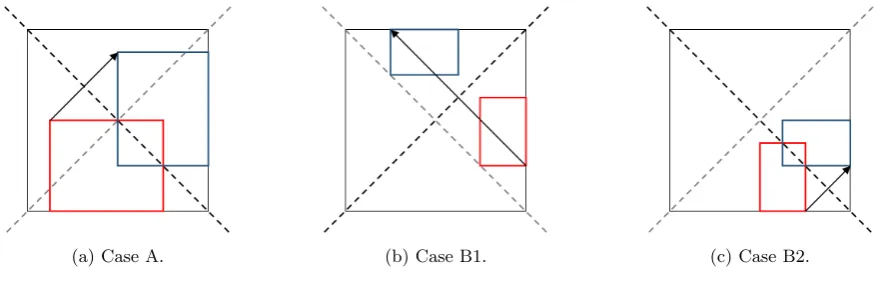
Fig. 1: The four quadrants of Hadamard matrix. We can further reduce the computation complexity using
the fact that Hadamard matrices are bisymmetric. Given a Hadamard matrix, we have four regions dissected by the left and right diagonal, namely top, left, right and bottom quadrant. For convention, we let the diagonal entries to be in both quad-rants. See Figure 1 for illustration, where the top four entries ”a” belong to both top and left quadrants, while the bottom four ”a” belong to both bottom and right quadrant.
Proposition 5 Given ak×k Hadamard matrixH, if all sub-matrices L with leading entry L[0,0] in the top quadrant are nonsingular, thenH is MDS.
Proof. It is known that the determinant of a matrix remains unchanged when it undergoes left or right diagonal reflection. Thus, it is sufficient to show that for any submatrix, it corresponds to some submatrix with the leading entry in top quadrant. This can be shown by looking at the reflection through the left and/or right diagonal. Consider the submatrices case by case:
• case B1: the leading entry is not in left quadrant and ending entry is in right quadrant. Through the right diagonal reflection, the ending entryL[l−1, l−1] of red submatrix is reflected to the leading entry in the top quadrant of the blue submatrix, see Figure 2b. Since the determinant does not change, the red submatrix will be nonsingular if the blue matrix is nonsingular.
• case B2: the leading entry is not in left quadrant and ending entry is in bottom quadrant. From Figure 2c, we see that through left diagonal reflection, the ending entry is now in the right quadrant, which is the case B1. ut
(a) Case A. (b) Case B1. (c) Case B2.
Fig. 2: Submatrices Reflections
Thanks to Propositions 4 and 5, our algorithm for checking the MDS property of Hadamard matrices is now much faster than a naive method. Namely, given a 2s×2s Hadamard matrix, the algorithm to test its MDS property can be as follows. First, we check that all entries are nonzero and forl = 2, . . . ,2s−1 we check that the determinant of l×l submatrices with leading entry in top quadrant is nonzero. If one submatrix fails, we outputFalse. Once all the submatrices are checked, we can outputTrue.
Using this algorithm as the core procedure for checking the MDS property, we can find the lightest-weight MDS involution Hadamard matrix by choosing a set of elements that sum to 1 with the smallest XOR count, permute the entries as mentioned in Section 4.1 and use this core procedure to check if it is MDS. If all equivalence classes of Hadamard matrices are not MDS, we swap some element in the set with another element with a slightly higher XOR count and repeat the process until we find the first MDS involution Hadamard matrix with the lowest possible XOR count. Eventually, we found the lightest-weight MDS involution Hadamard matrix of order 4 and 8 over GF(24) and GF(28), which can be found in Table 1 in Section 7. We emphasize that our results close the discussions on MDS involution Hadamard matrix of order 4 and 8, since our technique allows to take into account of all possible matrices.
5.3 Large dimension lightweight MDS involution matrices
The algorithm computation complexity grows exponentially with the matrix dimension, it is difficult to go to matrices of higher order. For that reason, we reduce the search space from Hadamard to Hadamard-Cauchy matrices, which guarantee the MDS property. Nevertheless, it is not feasible to generate and store all possible Hadamard-Cauchy matrices. For 16×16 Hadamard-Cauchy matrices over GF(28), by Lemma 5 we know there are almost a trillion distinct candidates. This is where the idea of equivalence classes comes in handy again. By Theorem 4, instead of storing over 9.7×10¹¹matrices, all we need is to find the 11811 equivalence classes. Even if memory space is not an issue, using Algorithm 1 to exhaustively search for all Hadamard-Cauchy matrices requires about 239.9iterations. In this subsection, we propose a deterministic and randomized algorithm that only takes on average of 216.9 iterations to find all the equivalence classes, which is equivalent to finding all possible Hadamard-Cauchy matrices.
First, we present two statements that are useful in designing the algorithm.
Lemma 7 Based on Algorithm 1, given a basis of s+ 1ordered elements {x1, x2, x22, ..., x2s−1, z}, any permutation
of the firsts elements {σ(x1), σ(x2), σ(x22), ..., σ(x2s−1), z} will form a Hadamard-Cauchy matrix that belongs to the
same equivalence class.
Proof. Since we are taking the span of the ordered set{x1, x2, x22, ..., x2s−1} and adding z to the span, it is obvious
that permuting{x2i}will only permute the order of the entries ofK. ut
Proposition 6 Given two positive integerssandr, wheres < r, doing exhaustive search through1≤x1< x2< x22 <
... < x2s−1 ≤2r and1 ≤z ≤2r is sufficient to find all possible equivalence classes of involutory Hadamard-Cauchy
Algorithm 2Finding all 2s×2sequivalence classes of involutory Hadamard-Cauchy matrices over GF(2r)/p(X). INPUT: an irreducible polynomialp(X) of GF(2r), integerss, rsatisfyings < randr >1.
OUTPUT: a list of equivalence classes of involutory Hadamard-Cauchy matrix.
procedureGenECofInvH-C(r, p(X), s)
compute the total number of equivalence classes,EC=Qs−1
i=0 2r−1−2i
2s−2i
initialize an empty set of arrayslist EC
while(sizeof(list EC)6=EC)do
selectslinearly independent elementsx1, x2, x22, ..., x2s−1 from GF(2r)/p(X) in ascending order
select elementzas linearly independent ofx1, x2, x22, ..., x2s−1
temp mat=ConstructH-C*(r, p(X), s,True, x1, x2, x22, ..., x2s−1, z)
if temp matis not a permutation of any matrix inlist EC then storetemp matintolist EC
end if end while returnlist EC
end procedure
Proof. Any linearly independent ordered set of elements {x1, x2, x22, ..., x2s−1} that are not in ascending order is
simply some permutation of a set in ascending order. By Lemma 7, it forms a Hadamard-Cauchy matrix of the same
equivalence class. ut
We describe our search method in Algorithm 2 and one can see that it uses most of Algorithm 1 as core procedure. We denote ConstructH-C* the procedure ConstructH-C from Algorithm 2 where the values x1, x2, x22, ..., x2s−1
andzare given as inputs instead of chosen in the procedure. We first chooses+ 1 linearly independent elements and apply Algorithm 1 to generate an involutory Hadamard-Cauchy matrix. We initialise an arraytemp mat and a list list ECto empty. Then,temp matis the matrix considered at the current iteration, it will be checked againstlist EC which is the list of equivalence classes of involutory Hadamard-Cauchy matrices that have been found. Iftemp mat is not a permutation of any matrix inlist EC, then a new equivalence class is found andtemp matwill be stored in list EC. When all the equivalence classes are found, we terminates the algorithm, which will dramatically cut down the number of iterations required.
From a representative of an equivalence class, one can obtain all the involutory Hadamard-Cauchy matrices of the same equivalence class through H-permutations. Note that the H-permutation is also applicable to non-involutory Hadamard-Cauchy matrices.
We remark that for 2×2 and 4×4 Hadamard-Cauchy matrices, any permutation of the equivalence class is still an involutory Hadamard-Cauchy matrix.
Notice that Algorithm 2 is a deterministic search for the equivalence classes. To further reduce the iterations needed, we propose to choose thes+ 1 elements randomly. Using this randomized search, it takes about 216.9iterations before finding all the equivalence classes. Once all the equivalence classes of involutory Hadamard-Cauchy matrices are found, we can check which matrix has the lightest-weight.
Using the randomized search algorithm, we found the lightest-weight involution Hadamard-Cauchy matrix of order 16 and 32 over GF(28), which can be found in Table 1.
6
Searching for MDS matrices
The disadvantage of using non-involution matrices is that its inverse may have a high computation cost. But if the inverse is not required, non-involution matrices might be lighter than involutory matrices. In this paper, we look at encryption only and do not consider the reuse of component for encryption/decryption (which can be studied in future work). Note that the inverse of the matrix would not be required for popular constructions such as a Feistel network, or a CTR encryption mode.
6.1 Circulant matrices
As the discussion on lightweight MDS circulant matrix is well-explored in [26], we focus on Hadamard-based matrix and extend the exhaustive search for from involutory to non-involutory lightest-weight MDS matrix.
6.2 Small dimension lightweight MDS matrices
that does not sum to 0, else it would be non-MDS, and apply the permutation method which is discussed at the end of Section 5.2 to check through all equivalence classes of Hadamard matrices.
6.3 Large dimension lightweight MDS matrices
After finding all the equivalence classes of involutory Hadamard-Cauchy matrices using the Algorithm 2, we can conveniently use this collection of equivalence classes to find lightest-weight non-involutory Hadamard-Cauchy matrix. That is to multiply by a nonzero scalar to each equivalence classes to generate all possible Hadamard-Cauchy matrices up to permutation. In this way, it is more efficient than exhaustive search on all possible Hadamard-Cauchy matrices as we eliminated all the permutations of the Hadamard-Cauchy matrices that have the same XOR count.
7
Results
We first emphasize that although in [20, 15] the authors proposed methods to construct lightweight matrices, the choice of the entries are limited as mentioned in Section 4.2. This is due to the nature of the Cauchy matrices where the inverse of the elements are used during the construction, which makes it non-trivial to search for lightweight Cauchy matrices7. However, using the concept of equivalence classes, we can exhaust all the matrices and pick the lightest-weight matrix.
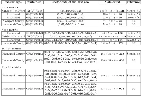
We applied the algorithms of Section 5 to construct lightweight MDS involutions over GF(28). We list them in Table 1 and we can see that they are much lighter than known MDS involutions like theKHAZADandANUBIS, previous Hadamard-Cauchy matrices [6, 20] and compact Cauchy matrices [15]. In Table 2, we list the GF(28) MDS matrices we found using the methods of Section 6 and show that they are lighter than known MDS matrices like the AES,
WHIRLPOOLand WHIRLWINDmatrices [17, 8, 7]. We also compare with the 14 lightweight candidate matricesC0to C13 for theWHIRLPOOL hash functions suggested during the NESSIE workshop [32, Section 6]. Both Tables 1 and 2 are comparing matrices that are explicitly provided in the papers. Recently, Guptaet al. [21] constructed some circulant matrices that is lightweight for both itself and its inverse. However we do not compare them in our table because their approach minimizes the number of XORs, look-up tables and temporary variables, which might be optimal for software but not for hardware implementations based purely on XOR count.
By Theorem 2 in Section 2, we only need to apply the algorithms from Section 5 and Section 6 for half the representations of GF(28) when searching for optimal lightweight matrices. And as predicted by the discussion after Theorem 1, the lightweight matrices we found in Tables 1, 2 and 3 do come from GF(28) and GF(24) representations with higher standard deviations.
We provide in the first column of the result Tables 1, 2 and 3 the type of the matrices. They can be circulant, Hadamard or Cauchy-Hadamard. The subfield-Hadamard construction is based on the method of [26, Section 7.2] which we explain here. Consider the MDS involutionM =had(0x1,0x4,0x9,0xd) over GF(24)/0x13 in the first row of Table 1. Using the method of [26, Section 7.2], we can extend it to a MDS involution over GF(28) by using two parallel copies of Q. The matrix is formed by writing each input byte xj as a concatenation of two nibbles
xj = (xLj||xRj). Then the MDS multiplication is computed on each half (y1L, yL2, y3L, yL4) = M ·(xL1, xL2, xL3, xL4) and (yR
1, y2R, yR3, yR4) =M·(xR1, x2R, xR3, xR4) over GF(24). The result is concatenated to form four output bytes (y1, y2, y3, y4) whereyj = (yLj||yRj).
We could have concatenated different submatrices and this is done in theWHIRLWINDhash function [7], where the authors concatenated four MDS submatrices over GF(24) to form (M
0|M1|M1|M0), an MDS matrix over GF(216). The submatrices are non-involutory Hadamard matrices M0 = had(0x5,0x4,0xa,0x6,0x2,0xd,0x8,0x3) and M1 = (0x5,0xe,0x4,0x7,0x1,0x3,0xf,0x8) defined over GF(24)/0x13. For fair comparison with our GF(28) matrices in Ta-ble 2, we consider the correspondingWHIRLWIND-like matrix (M0|M1) over GF(28) which takes half the resource of the originalWHIRLWINDmatrix and is also MDS.
The second column of the result tables gives the finite field over which the matrix is defined, while the third column displays the first row of the matrix where the entries are bytes written in hexadecimal notation. The fourth column gives the XOR count to implement the first row of then×nmatrix. Because all subsequent rows are just permutations of the first row, the XOR count to implement the matrix is just ntimes this number. For example, to compute the XOR count for implementing had(0x1,0x4,0x9,0xd) over GF(24)/0x13, we consider the expression for the first row of matrix multiplication 0x1·x1⊕0x4·x2⊕0x9·x3⊕0xd·x4. From Table 8 of Appendix D, the XOR count of multiplication by0x1,0x4,0x9and0xdare 0, 2, 1 and 3, which gives us a cost of (0 + 2 + 1 + 3) + 3×4 = 18 XORs to implement one row of the matrix (the summand 3×4 account for the three XORs summing the four nibbles). For the subfield construction over GF(28), we need two copies of the matrix giving a cost of 18×2 = 36 XORs to implement one row.
7
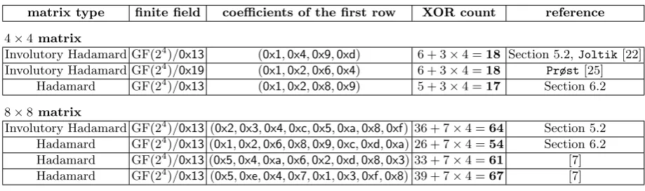
We also applied the algorithms from Section 5 and Section 6 to find lightweight MDS involution and non-involution matrices of order 4 and 8 over GF(24), these matrices are listed in Table 3. By Corollary 2 and the structure of Hadamard matrix, the first row of an MDS Hadamard matrix must be pairwise distinct. Therefore, there does not exist Hadamard matrix of order larger than 8 over GF(24). Due to the smaller dimension of the finite field, the XOR counts of the matrices over GF(24) are approximately half of those over GF(28).
The application of our work has already been demonstrated in Joltik, a lightweight and hardware-oriented au-thenticated encryption scheme that uses our lightweight MDS involution matrix of order 4 over GF(24) with XOR count as low as 18. On the other hand, the diffusion matrix fromPrøst [25] was designed with a goal in mind to minimise the number of XOR operations to perform for implementing it. By Theorem 2 in Section 2 and reference to Table 4, we observe that these two matrices are in fact the counterpart of each other in their respective finite fields. Thus, they are essentially the same lightest matrix according to our metric.
In addition to Table 3, the subfield-Hadamard constructions in Tables 1 and 2 also capture the lightweightness of our GF(24) matrices, and we show that our constructions are lighter than known ones. For example, the GF(24) matricesM0andM1used in theWHIRLWINDhash function has XOR count 61 and 67 respectively while our Hadamard matrixhad(0x1,0x2,0x6,0x8,0x9,0xc,0xd,0xa) has XOR count 54.
With our work, we can now see that one can use involutory MDS for almost the same price as non-involutory MDS. For example in Table 1, the previous 4×4 MDS involution from [20] is about 3 times heavier than theAESmatrix8; but in this paper, we have used an improved search technique to find an MDS involution lighter than the AESand
ANUBISmatrix. Similarly, we have found 8×8 MDS involutions which are much lighter than theKHAZAD involution matrix, and even lighter than lightweight non-involutory MDS matrix like theWHIRLPOOLmatrix. Thus, our method will be useful for future construction of lightweight ciphers based on involutory components like theANUBIS,KHAZAD,
ICEBERGandPRINCEciphers.
Table 1: Comparison of MDS Involution Matrices over GF(28)
(the factor 2 appearing in some of the XOR counts is due to the fact that we have to implement two copies of the matrices)
matrix type finite field coefficients of the first row XOR count reference
4×4matrix
Subfield-Hadamard GF(24)/0x13 (0x1,0x4,0x9,0xd) 2×(6 + 3×4) =36 Section 5.2 Hadamard GF(28)/0x165 (0x01,0x02,0xb0,0xb2) 16 + 3×8 =40 Section 5.2 Hadamard GF(28)/0x11d (0x01,0x02,0x04,0x06) 22 + 3×8 =46 ANUBIS[5] Compact Cauchy GF(28)/0x11b (0x01,0x12,0x04,0x16) 54 + 3×8 =78 [15] Hadamard-Cauchy GF(28)/0x11b (0x01,0x02,0xfc,0xfe) 74 + 3×8 =98 [20]
8×8matrix
Hadamard GF(28)/0x1c3 (0x01,0x02,0x03,0x91,0x04,0x70,0x05,0xe1) 46 + 7×8 =102 Section 5.2 Subfield-Hadamard GF(24)/0x13 (0x2,0x3,0x4,0xc,0x5,0xa,0x8,0xf) 2×(36 + 7×4) =128Section 5.2 Hadamard GF(28)/0x11d (0x01,0x03,0x04,0x05,0x06,0x08,0x0b,0x07) 98 + 7×8 =154 KHAZAD[6] Hadamard-Cauchy GF(28)/0x11b (0x01,0x02,0x06,0x8c,0x30,0xfb,0x87,0xc4) 122 + 7×8 =178 [20]
16×16matrix
Hadamard-Cauchy GF(28)/0x1c3 (0x08,0x16,0x8a,0x01,0x70,0x8d,0x24,0x76, 258 + 15×8 =378 Section 5.3 0xa8,0x91,0xad,0x48,0x05,0xb5,0xaf,0xf8)
Hadamard-Cauchy GF(28)/0x11b (0x01,0x03,0x08,0xb2,0x0d,0x60,0xe8,0x1c, 338 + 15×8 =458 [20] 0x0f,0x2c,0xa2,0x8b,0xc9,0x7a,0xac,0x35)
32×32matrix
Hadamard-Cauchy GF(28)/0x165
(0xd2,0x06,0x05,0x4d,0x21,0xf8,0x11,0x62,
610 + 31×8 =858 Section 5.3 0x08,0xd8,0xe9,0x28,0x4b,0xa6,0x10,0x2c,
0xa1,0x49,0x4c,0xd1,0x59,0xb2,0x13,0xa4,
0x03,0xc3,0x42,0x79,0xa0,0x6f,0xab,0x41)
Hadamard-Cauchy GF(28)/0x11b
(0x01,0x02,0x04,0x69,0x07,0xec,0xcc,0x72,
675 + 31×8 =923 [20] 0x0b,0x54,0x29,0xbe,0x74,0xf9,0xc4,0x87,
0x0e,0x47,0xc2,0xc3,0x39,0x8e,0x1c,0x85,
0x58,0x26,0x1e,0xaf,0x68,0xb6,0x59,0x1f)
8