Parameter estimation of continuous-time point processes: Serial dependency and neural applications

Parameter Estimation of Continuous-time Point Processes:

Serial Dependency and Neural Applications

Chia-yee Jerry Liu

Institute of Statistics Mimeograph Series No. 2203T

Panmeter EstimationofContinuowt-time PointProcesses:SerialDependencyandNeural Applications

Chia--yeeJerry Liu

(Under the directionofCharlesEugene Smith.)

Dept. ofStatistics, NorthCaroJiDaState University Abstract;

Three approaches to removing the serial dependence or lack of independence between interspike intervals are examined in simulated and in cat auditory nerve data. Stationary portions of the data are located by windowing firing rates and a runs-test. The independence of intervals is examined by correlograms, a periodogram test and by conditional interval plots. Auditory-nerve fiber spike-trains were found to have a negative first order serial correlation coefficient and a corresponding negative slope in the conditional mean plots. Removal of the negative dependence (long interval follows short and vice versa) was validated by the conditional interval histograms. The three possible causes of the serial dependence considered here are: a location shift, scale shift, and shape parameter change with the conditioning interval in the conditional mean plot. The scale shift procedure seems most appropriate for the auditory-nerve fiber spike-trains examined. Previous work (e.g., Johnson et.· al., 1986, Hearing Res. 21:135-159) has shown negative serial dependence in another part of the auditory system, LSO units.

PARAMETER ESTIMATION OF CONTINUOUS-TIME POINT PROCESSES: SERIAL

DEPENDENCY AND NEURAL APPLICATIONS

by

CHIA-YEE JERRY LIU

A thesis submitted to the Graduate Faculty of

North Carolh.ta State University

"

in partial fulfillment of the

requirements for the Degree of

Doctor of Philosophy

DEPARTMENT OF STATISTICS

Raleigh

1991

APPROVED BY:

ACKNOWLEDGEMENT

Itismy pleasure to express my gratitude for'the help and encouragement received in the course of the work so far accomplished.

The experimental spike-traindata sets were obtained by the c:ourtesy of Professor Eric .Tavel of Duke University Medical Center, Durham, North Carolina. His friendliness is deeply appreciated.

The research work was financially supported by the Office of Naval Research (Grant Number: NOOOl4-90-.T-1646-1).

Professor Charles Smith, serving as my maJor advisor as well as a friend, deserves every thank.

, .

Never'could I have become what I am now without his superb professional guidance, extreme patience, and constant generous encouragement. The scenes of he and I working together in the 3-a.m. silence are imprinted in my mind, forevtlr.

•

•

TABLE.QlCONTENTS

List ofTables

List ofFigures

List ofSymbols

Chapter Ilntrodudolynotes:~traiDs,the modeling,

andbasicstatisticalCOD8ideratiODS 1.1Singleneuralspike-trains

1.2 Stochastic pOintPIOCeS8e8and its relati.cmshiptospike-trains 1.3Roleofstatistic:a in spike-trainanalysis

1~4Tests forstationarityandfor renewalproperty

1.5A. timglanceatthe whiteDing procedures 1.6 Driven spike-trains

Chapter2 Pilot study on simulatedspontaneous spike-trains 2.1The intensity approach

2.2 Data preparationsteps 2.3Diagnostic graphical tools 2.4 The renewalcase-NERVEI 2.5 The nonrenewal case-NERVE2 2.6 Ananalytical example-LS7712 2.7 Discussion

Chapter3More on the whitening procedures 3.1 Ananalytical illustration

3.2 The renewal gamma spike-train 3.3Thecorrelatedgamma spike-trains

3.3.1 Loc:ationshift

3.3.2Scale shift

3.3.3Shape change

3.4 Anothersetofgammaspik~trains

3.5 Results

Chapter4Spike-trains from experimental animals 4.1 The experiment

4.2Basic observations

v vi

1 2 3 5 10 13 15

17 17 19 21 25 26 28 36

38 39 43 43 44 46 47 49 51

4.3Eumplee-ca&auditory-llen'fI~spike-baina

4.4DiacusBicm

Chapter5Driven spike-baina 5.1 POIdsyDapticmodulation 5.2 PlesyDapticmodulation 5.3Compariarmaandcomments 5.4 SugesU.ouaforfurtherneeazch

Appeadic:es

Tables

FigmeLegend

Figures

References

66

•

59

61 61 63 65

66

70

73

81

95

183

•

•

Table 2.1 Results of MLE for NERVE1

Table 2.2 Results of MLE for whitened NERVE2

Fie. 1.1 Schematic diagram of a typical neuron Fie. 2.1 AIcorithm flow-chart

Fie. 2.2 Conditional plots of NERVE1

Fie. 2.3 Conditional interval histograms of NERVE1

Fig. 2.4 Hazard rate plot of NERVE1 with estimated intensity function Fig. 2.5 Conditional plots of NERVE2

Fie. 2.6 Conditional interval histograms of NERVE2 Fie. 2.7 Conditional plots of whitened NERVE2

Fie. 2.8 Conditional interval histograms of whitened NERVE2

Fie. 2.9 Hazard rate plot of whitened NERVE2 with estimated intensity function Fie. 2.10 Conditional plots of L57712

Fig. 2.11 Conditional interval histograms of L57712 Fie. 2.12 Interval histogram of L57712

Fig. 2.13 Conditional plots of AR(l) whitened L57712

Fig. 2.14 Conditional interval histograms of AR(l) whitened L87712 Fig. 2.15 Conditional plots of variable transformation whitened L87712

Fig. 2.16 Conditional interval histograms of variable transformation whitened L87712

Fig. 3.1 Conditional plots of original NERVE2

Fig. 3.2 Analytical illustration of 3 types of serial correlations

Fig. 3.3 Conditional interval histograms with location type correlation Fig. 3.4 Conditional interval histograms with scale type correlation Fig. 3.5 Conditional interval histograms with shape type correlation

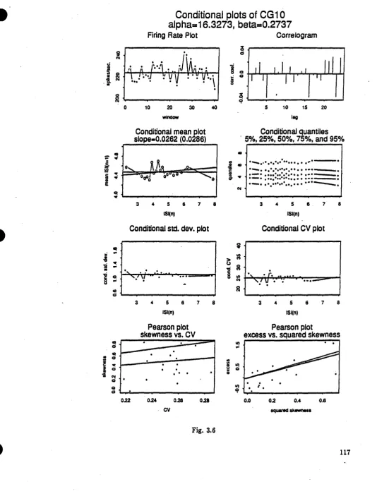
Fig. 3.6 Conditional plots of renewal gamma spike-train with n=2000 (CG10)

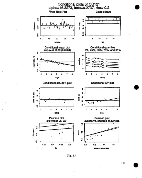
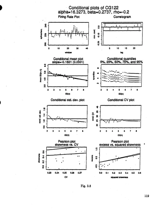
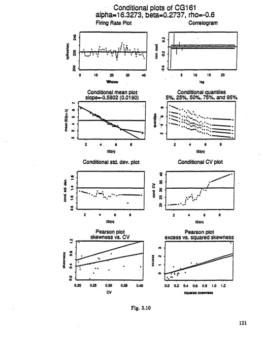
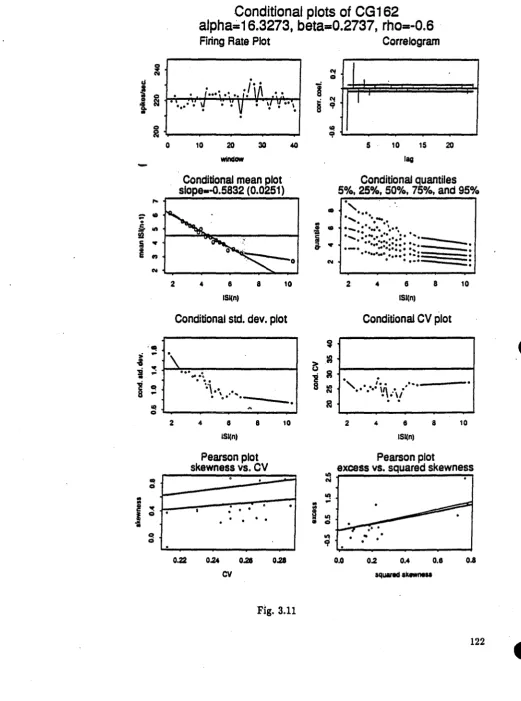
Fig. 3.7 Conditional plots of location shifted gamma spike-train with n=2000, p= - 0.2 (CG121) Fie. 3.8 Conditional plots of scale shifted gamma spike-train with n=2000, p= - 0.2 (CG122) Fig. 3.9 Conditional plots of shape changed camma spike-train with n=2000, p= - 0.2 (CG123) Fie. 3.10 Conditional plots of location shifted gamma spike-train with n=2000, p= - 0.2 (CG161) Fie. 3.11 Conditional plots of scale shifted camma spike-train with n=2000, p= - 0.2 (CGI62) Fig. 3.12 Conditional plots of shape changed camma spike-train with n=2000, p= - 0.2 (CG163) Fig. 3.13 Conditional plots of renewal gamma spike-train with n=10000 (CG50)

Fie. 3.14 Conditional plots of location shifted gamma spike-train with n=10000, p= - 0.6 (CG521)

Fig. 3.15 Conditional plots of scale shifted gamma spike-train with n=10000, p= - 0.6 (CG522) vi

•

Fig. 3.16 Conditional plots of shape changed gamma spike-trainw~thn=10000, p= - 0.6 (CG523) Fig. 3.17 Conditional plots of location shifted gamma spike-train with n=10000, p= - 0.6

(CG561)

Fig. 3.18 Conditional plots of scale shifted gamma spike-train with n=10000, p= - 0.6 (CG562) Fig. 3.19 Conditional plots of shape changed gamma spike-train with n=10000, p= - 0.6 (CG563) Fig. 3.20 Conditional interval histograms of CG50, renewal

Fig. 3.21 Conditional interval histograms of CG521, location shift Fig. 3.22 Conditional interval histograms of CG522, scale shift Fig. 3.23 Conditional interval histograms of CG523, shape change Fig. 3.24 Conditional interval histograms of CG561, location shift Fig. 3.25 Conditional interval histograms of CG562, scale shift Fig. 3.26 Conditional interval histograms of CG563, shape change Fig. 3.27 Conditional plots of renewal gamma spike-train (CG50A) Fig. 3.28 Conditional plots of CG561A

Fig. 3.29 Conditional plots of CG562A Fig. 3.30 Conditional plots of CG563A

Fig. 3.31 Conditional interval histograms of CG50A, renewal Fig. 3.32 Conditional interval histograms of CG561A, location shift Fig. 3.33 Conditional interval histograms of CG562A, scale shift Fig. 3.34 Conditional interval histograms of CG563A, shape change Fig. 3.35 Summary plots of CG50A, CG561A, CG562A, CG563A

Fig. 4.1 Post-stimulus time (PST) histograms of cat cochlear nucleus spike-trains Fig. 4.2 Post-stimulus time (PST) histograms of cat auditory-nerve fiber spike-trains Fig. 4.3 Period histograms of cat cochlear nucleus spike-trains

Fig. 4.4 Period histograms of cat auditory-nerve fiber spike-trains Fig. 4.5 Interval histogram of AUDO

Fig. 4.6 Interval histogram of AUDIO Fig. 4.7 Interval histogram of AUD20

Fig. 4.8 Conditional plots of cat auditory-nerve fiber spike-train (0 dB SPL) Fig. 4.9 Conditional plots of cat auditory-nerve fiber spike-train (10 dB SPL) Fig. 4.10 Conditional plots of cat auditory-nerve fiber spike-train (20 dB SPL)

Fig. 4.14 Conditional plots of cat auditory-nerve fiber spike.train at lag 2 (0 dB 8Pt) Fig. 4.15 Conditional plots of cat auditory-nerve fiber spike.train at lag 2 (10 dB 8Pt) Fig. 4.16 Conditional plots of~tauditory-nerve fiber spike.train at lag 2 (20 dB 8Pt) Fig. 4.17 Conditional plots of cat auditory-nerve fiber spike.train at lag 3 (10 dB 8Pt) Fig. 4.18 Conditional interval histograms of whitened cat auditory-nerve fiber spike.train

(0 dB 8Pt)

Fig. 4.19 Conditional interval histograms of whitened cat auditory-nerve fiber spike.train (10 dB 8Pt)

Fig. 4.20 Hazard rate plot of whitened cat auditory-nerve fiber spike.train (0 dB 8Pt) with estimated intensity function

Fig. 4.21 Hazard rate plot of whitened cat auditory-nerve fiber spike.train (10 dB 8Pt) with estimated intensity function

Fig. 4.22 Interval histogram of reproduced AUDO Fig. 4.23 Interval histogram olreproduced AUDIO

Fig. 4.24 Conditional interval histograms of reproduced AUDO Fig. 4.25 Conditional interval histograms of reproduced AUDIO Fig. 4.26 Conditional plots of whitened AUD20

Fig. 4.27 Conditional plots (at lag 2) of the intermediate spike.train of AUDO

Fig. 5.1 Period histogramsofsimulated driven spike.trains

e·

Lii.

9f

Symbols

Nt :count of occurrences up to time tof a point process (random variable)

lit :count of occurrences up to time tof a point process (observed value)

"t :vector of occurrence times up to time tof a point process

"II. :vector of occurrence times upto the last occurrence t

'Ti :the ~thinterapike-interval of a spike-train (point process) Pi : ~th-orderPearson's correlation coefficient

~ : intensity of a homogeneous Poisson process; intensity function of a point process

~ : asymptotic firing rate

cr : recovery shape constant; shape parameter of a ganima distribution

{J : recovery time constant; scale parameter of a gamma distribution

It is widelyaccept~ that sequences of nerve impulses(alsoknown as action potentials, or simply, spike-trains) are the main means of transmitting relevant biological information in the nervous system. These sequences reflect the cellular activities that underlie the neuron's spike-generating mechanism. The production of an impulse by a neuron is considered to be the result of the electro-chemical activity that takes place at a specialized region of the neuron called the spike initiation site. One w~y to envision the mechanism producing the spike is as a voltage threshold crossing. A spike-train composed of these temporally distributed impulses is said to be a spontaneous spike-train if no stimulus is present during the period of observation. Otherwise, it is called a stimulated, or driven, spike-train. The characteristic features shared by all spike-trains: randomness in the temporal pattern, indistinguishability in the shape and waveform of the spikes, and relatively short duration of each spike, lead to stochastic point process modeling. Statistical analysis plays a critical role when relating these probabilistic models to actual or simulated data.

There have been two major approaches to validate a model via simulation. One uses various moments of the data and the other uses th~ intensity function description of a point process. The first one,. sometimes called the moment method, seeks to reproduce a number of moments of the observed spike-train through simulation. The second one, the so-called intensity function description of a point process, tries to reproduce the spike-train temporal pattern through simulation with a hypothesized intensity. Both approaches rely on statistical inference methodology and lead to parameter estimation and hypothesis testing. This thesis will emphasize the parameter estimation aspect.

The aim of this thesis is to present an algorithm to analyze neural spontaneous or maintained response spike-trains from the intensity point of view. As part of the algorithm, the correlation structure of the interspike intervals of the spike-trains were extensively examined. If

results obtained from the studyofits spontaneous counterpart.

The rest of this chapter will serve as a brief tutorial on spike-trains, the modeling schemes, and the basic statistical considerations. Some of the details willbe examinedfurther in the following chapters. Chapter 2 performs an analysis on three simulated spontaneous spike-trains as a pilot study of the algorithm. Chapter 3 presents a more detailed discussion on the cone1ation types of spike-trains. Chapter 4 contains an analysis on spike-trains of cat cochlear nucleus and auditory-nerve fiber. Chapter 5 extends the results from spontaneous spike-trains to simulate driven spike-trains for a sinusoidal stimulus. The correlation structure and the periodicities of the driven spike-trains were examined.

1.1 Singleneul'Ollspik..trains

The material presented here is a simplified description of how a neuron functions within the nervous system.It is from a statistician's point of view and an effort has been made to avoid excessive physiological jargon.

An electro-chemical impulse from a neuronistermed a spike or a discharge. A spike-train is referred to a sequence of identical spikes characterized by its occurrence times relative to the onset of observation. More details can befound in Perkel et al., 1967, Stein, 1972, Fienberg, 1974, Yang and Chen, 1978,

Lee,

1979, and Tuckwell, 1988.

The basic structural unit of the vertebrate nervous systemisa neuron whichis an animal cell with specialized electrical properties. Neurons transmit signals either to or from the brain or the spinal cord. They can be classified, according to their functions into three types: sensory, interneuron, and motor. Despite the fact that neurons differ greatly in size, shape, and physiological functions, they are all recognized as consisting of four parts: soma, dendrites, axon, and synapses as shown in Fig. 1.1. The neuron's membrane is selectively petmeable to ions such as Na+ and K+ and without stimulation tends to maintain a constant potential called the resting potential. When signals from other neurons are received through the synapses, the membrane is said to be polarized. An input signal is classified as excitatory (inhibitory) if it produces a depolarization (hyperpolarization). Said another way, excitatory inputs move the membrane potential closer to the voltage threshold, while the inhibitory ones move it farther away.

integrator", i.e., the linear operator dV/dt +V/rn' where Vis the voltage at the spike initiation site and rn is the membrane time constant (c.f., tirst-order autoregressive (AR(I» time series models). The membrane potential level moves upward when depolarized, and downward when hyperpolarized. Instead of staying fixed between polarizations, the membrane potential decays toward ita resting potential because of "leakage" through the membrane. The moment the threshold is exceeded, the neuron produces a spike discharge (action potential) at the spike initiating site and sends it down the axon to the connecting neurons. The postspike membrane potential returns to a reset level which may be slightly lower than the resting potential.

Following each discharge, the neuron becomes temporarily "paralyzed" for a period of time which is termed the absolute refractory period or simply the dead-time. During this time, all input signals are ignored because the summing mechanism is "dead", hence no discharge will occur. The so-called relative refractory period comes right after the dead-time. The threshold level is relatively higher than usual during the relative refractory period and thus spikes are less likely to be produced. For some neurons, the lengths of these two periods have been considered as random variables (e.g., Teich and Saleh, 1981).

The spike-trains produced by a neuron are either due to its spontaneous activity or its response to stimuli. The former can be considered the background neuronal activity as stated in Tuckwell, 1988, while the latter can be viewed as the interaction of the spontaneous activity and the effect attributed to the stimulus.

Since the spikes observed have approximately the same waveform and short duration (Stein, 1972), the spike-trains of vertebrate neurons can be modeled as stochastic point processes for which occurrence times, or equivalently, interspike intervals, suffice to characterize the spike-trains. Note that when dealing with different types of neurons, the details in the models may be different, e.g., the time constantrn may be different.

1.2 Stochastic point~and their relationshiptospike-trains

A stochastic point process is a mathematical model for a series of point events which evolve randomly in a continuum. The point events are identical except for their locations in the continuum and it is assumed for convenience that no two events share the same location (termed "orderliness" by the above literature). Since we are dealing with temporal data throughout the thesis, the continuum spaceXis considered exclusively to be the semi-infinite time interval T=(t; t~

OJ.

The locations thus are termed occurrence times and are denoted by the vector w=(wl'

w2'''')where wo=Ounless otherwise specified.

The information one gains through observing a particular realization of a point processis

the sequence of occurrence times 'W_t up to time t, or equivalently, the inter-arrival times T=(r1,r2'''')' whererlc= wlc - wlc_l'for k~1. The history of a realization of a point process up to time t contains nt, the number of events which occurred prior to t, and'Wt=(w_1, w2,,,,,w_{n ),}and is

t

denoted by H_{t •} The Poisson process, a well-known and useful point process, is used below to introduce the definition of the intensity function.

Let {Nt; t~O} denote a point process on T={t; t~O}. Let n_t be the number of events observed up to time t and let 'W_t=(wl,w2,,,,,w_{n )} be the corresponding occurrence times. Suppose

t

that

and

Pr{Nt

+

6 - Nt

>

11

HJ= 0 (6)

for some 6

>

0, where

lim 0 £6)=0.

6-0 u

Then if A(t; HJ=Ao,anonnegative constant, (Nt; t~

OJ

is called a homogeneous Poisson process. If A(t; Ht)=!(t), some nonnegative function depending only on t, {Nt; t~

OJ

is called an inhomogeneous Poisson process. If A(t; HJcannot be relieved of its dependence on tor _{Ht, {Nt;} t~

OJ

is called a self-exciting point process (Snyd.er, 1975, p. 238). In all three cases, A(t; HJis

renewal property, i.e., each event has no aftereffect on the following ones. This definition of an intensity function conditioned on the history of the point process will be considered further in Chapter 2.

From a particular realization of a point process, one seeks to specify the underlying point process. The complete specification of a point process {Nt; t~OJ may be achieved via the specification of its intensity function ).(t; HJ, t~0, or the joint distribution of w_{t '} the random vector of occurrence times. Also note that when multiple occurrences are excluded, 'r, the vector

of inter-arrival times, is equivalent to w_{t •} When applied to physical phenomena such as spike-train analysis, the intensity approach is the one primarily employed.

An observed spike-train can be treated as a realization of a point process when the differences in the waveform and the amplitude of individual spike discharges are ignored. The occurrence time of a spike is then taken tobe the instance of the peak excursion of the membrane potential. Because of the random timing of the spike-trains, the stochastic point process model is appropriate in modeling spike-trains.

A biological justification for regarding the output from a single nerve cell as a point process can be found in Stein, 1972. The main criterion, based on electrical circuit models, seems to be that the nerve fibers are long and thin enough to preclude passive transmission, i.e., transmission without action potentials. This criterion appears to be met in the major nerve tracts of most higher animals.

The goal of statistical inference related to spike-train analysis is to disclose information about the generating mechanism from presynaptic input to postsynaptic output of a single neuron, the interconnections and interactions among a number of neurons, and the structure and function of the entire nervous system. I will focus on the first topic in this thesis. Chapter 5 briefly examines the predictive use of statistical spike-train analysis.

1.3 Roleof mtistics in spik.train IInlllysis \

random variable defined by the ft-th interspike interval, while

T,.

isthe realization oflSI,..

When dealing with a recorded realization of a point process{Nt; t~OJ, the first concern

is whether it is a renewal process, due to the mathematical tractability of renewal processes. If

what underlies a spike-trainisindeed a renewal point process, then its ISrs are independent and identically distributed (iid), i.e., the point process evolves identically without aftereffects. Consequently, the probability density function (pdf)

I.,.(t),

or the cumulative distribution function (cdt) F.,.(t)= I1J(I)dl of the lSI's completely specifies the process. Furthermore, because of the correspondence

w"

St ifand onlyif Nt~k, k=1,2,...,

it can be seen that' the process {Nt; t~O} and the. evolution {w_{n ;} n~l} are directly

interchangeable. Several interesting and useful lSI pdf's arediscussedin Tuckwell, 1988.

The second concern is stationarity. Unless otherwise specified, stationarity means wide sense stationarity throughout this thesis. A process {X(t); t~O} is said to be (wide sense) stationary if

EX(t)=JJ

and

EX(t)X(t+v)=g(v)

for all tET=[0,00), v ER. Reasons to examine whether point processes are stationary or not are twofold: the mathematical tractability and that we want to extract stationary portions of an observed spike-train. It is widely accepted that spontaneous spike-trains can be modeled as stationary point processes (e.g., Kiang et al., 1965).

It is clear that a renewal process is automatically stationary according to its definition. But in order to enlarge the capability of modeling spike-train phenomena, the definitions are altered when those two properties are put into combination. Two classes of point processes are defined as follows. A point process is called a stationary renewal (SR) point process if it is a stationary point process with independent lSI's, i.e., a stationary point process evolves without aftereffects. A point process is called a nonstationary renewal (NSR) point I?rocess if it is a nonstationary point process with independent lSI's, i.e., it is not stationary but still evolves without aftereffects.

Following the definition of the intensity function in the last section, the intensity fUIiction of a stationary renewal(SR) point process canbesimplified tobe

>.(t; Ht)=f(t - w_{n ),}

i.e., the dependence of the intensity function on tisonly through the difference between the time instant t and the occurrence time of the latest event w_{n '} where f(.) is a nonnegatiYe function.

t

The intensity function of a nonstationary renewal(NSR)point processisof the form >.(t: HJ:f(t, t -w_{n /}

where f(.,. )isa nonnegative function of two variables. Via the use of intensity functions, we are able to concentrate modeling efforts on the determination of the function f, either parametrically or nonParametrically.

A well-known family of point processes is the Poisson family. Itisimmediately seen that a homogeneous Poisson process of intensity

>.

is a stationary renewal process with lSI pdf

f-r(t)=>.e->.t, for t>O. And an inhomogeneous Poisson process is a nonstationary renewal point process since there is no aftereffects. When considered within the framework of self-exciting point prOCesses, both stationary renewal and nonstationary renewal point prOCesses have intensity functions involving their histories only as far back as the most recent occurrence, are thus called

I-memory self-exciting point processes (Snyder, 1975, p. 257).

There are many empirical tools which help in different aspects of identifying a point process. A brief review is now presented that stresses the intensity point of view.

Interspike interval

.usn

histogram Suppose there are N observed lSI's, denoted by ri'

i=l,I, ...,N. And there are Jbins of equal width 6. Let N_j be the number of r/s that fall in the interval ((j-1)6, i6J, i=1,D,...,J.The lSI histogram is the piecewise flat curve

fj=Nj/N, i=1,D, ...,J,

plotted against the time axis.

The lSI histogram is actually the relative frequency histogram of the lSI's.Itis one of the first-order statistics of the spike-train and in the limit it serves as an unbiased estimate of the lSI pdf provided that the process is renewal. If either one of the requirements of being renewal fails to hold, then inferences based solely on the lSI histogram can be greatly misleading. When the underlying point process is indeed renewal, then lSI histogram characterizes the point process to within a time interval 6.

Hazard

m!!

The hazard function h(t)of the lSI's is defined to be

h(t)=f-r(t)/{1- Fr(t)J,

e-histogram as

,-

. 1

1&,-=1/[1-

E

I,), i=1,1,... J.

k=1

The hazard rate can always be evaluated from the lSI histogram.

When a point process is renewal, then its hazard function and intensity function are identical (Snyder, 1975).This can be seen as follows:

1&(t)=I.,.(t)/[1- FT(t)J

=).(t

I

H_{t) •} exp(- J~).(s

I

HJds) / [1- (1-exp(- J~).(s

I

HJds))J

=).(tl HJ.

Post-stimulus·

Bn:ll

!ESIl

histogram When stimuli are applied to a neuron, the spike-train produced by the neuron may no longer be stationary. The lSI histogram is then insufficient to illustrate the behavior of the spike-train. The PST histogram incorporates the presence of the stimuli by setting each onset of the stimuli as the time origin, t=O, and expressing the vertical axis of the histogram as an instantaneous rate in spikes per second. The purpose of the PST histogram is to measure the temporal variation of the rate of discharge of the neuron under stimulation (Johnson et al., 1986). The method of plotting the PST histogram can be found in Johnson, 1978. In the same article, it is stated that "the PST histogram can serve as an unbiased estimate of the ensemble average of a spike-train intensity". Some PST histograms of cat auditory-nerve fiber spike-trains will be shown in Chapter 4.

Serial correlogram

m

conditional!lWYl§ The serial correlogram is a measure of the linear serial dependence of lSI's. Conditional means are used to provide a graphical illustration of the serial dependence and can indicate a lack of linearity. Both of them are second-order statistics of the spike-train under study, used especially when it is unknown whether or not the spike-train is evolving without aftereffects.

where

N-i

'F';=l

E

'Ti

J/(N-

i),

i=l

N-i

':f'.'=(

E

'T.

+ .

J/(N-

i),

, i = l ' ,

;,2being the ordinary sample variance.

It is known that, given that the lSI's are independent, the sample correlation coefficient of order ;, p;, has an asymptotic normal distribution with mean zero and variance

l/(N-l) for large N. Roughly speaking, the closer

ci

is to zero, the more likely that the lSI's are uncorrelated. The difficulty of using thecorrelogram is that the confidence limits arebaaed on the asymptotic standard deviations of individual correlation coefficient. And the correlation

coeffi~ents measure only the linear correlation of the observations (Klemm and Sherry, 1981).

The criterion to judge whether an observed spike-train has uncorrelated lSI's is derived from this fact and will be outlined in the following section.

The conditional means are E{ISIn

+

1

1'T,J,

n=l,

e,...,

N.

There are two ways to plot the graph of the empirical conditional means against the conditioning lSI. The fIrSt one is to bin the time axisequally, then group the lSI's according to bins in which the previous lSI's fall. The group means are plotted against the midpoints of the bins. The second method uses a different way of binning when the discharge rate is not too high. Equal number of lSI's are grouped into the same bin such that each calculated group mean is an average of a same number of lSI's. It is like plotting p%-quantile conditional means against the midpoints of the corresponding p%-quantile intervals where

p _ 100

- no. of bins'

Only the second method was used throughout this thesis since the data sets used were not large and the firing rates were not too high.

Theserial correlogram and conditional mean plot are employed throughout the thesis to quantifying the serial correlation that might be in a spike-train. A serial correlation has been observed to exist in spike-trains produced by a number of types of neurons (e.g., Johnson et al., 198.6, Goldberg et al., 1964, Goldberg and Greenwood, 1966). It is recognized as an integral part

ofboth the statistical and biological properties of a spike-train (SaIIlpath and Srinivasan, 1977, Klemm and Sherry, 1981). The importance of the serial correlation in the interspike intervals of spike-trains will again be emphasized at the end of this thesis.

1.4 T. .formtionarityandforrenewalpropetty

Mathematically rigorous results in justifying point processes are desired not only to identify the target point ,process but also to extract segments possessing certain properties, e.g., stationarity, from the observed spike-train. A number of tests will be outlined in this section. They are divided into three categories, namely: stationarity, independence of lSI's, and the renewal property. The test results are used to select the appropriate modeling scheme.- Other specific tests are omitted here and will be brought up when necessary. Detailed discussion of the test procedures can be found in Cox and Lewis, 1966, Correia and Landolt, 1977, Landolt and

Correi~,1978,Yang and Chen, 1978,and Tuckwell, 1988.

I. Stationarity

It is known that spontaneous spike-trains are stationary (e.g., Fienberg, 1974). Also, while a persistent stimulus is applied, the spike-train will reach a relatively steady rate of discharge after a transient period. This is called the maintained response. Hence the preliminary step to test for stationarity is to roughly scan through the entire spike-train, locate and disregard those obviously nonstationary portions to avoid distorting the test results. The PST histogram is a good indicator for doing so. The test for stationarityusedin this thesis is listed as follows (c.f. Appendix B):

Wald-Wolfowitz runs test

and -'s, and n+ and n_ denote the numbers of +'s and -'s, respectively. For example, a sequence of --++++-+-- gives r=5, n+=5, and n_=5. Then, provided that n=n++n_ is

large enough,

Z=(/r-prl-l/~)/SD,.,

where

pr=l+(ln+. n_)/n,

and

SDr=( (Pr-1)(Pr-

~)/(n+l)//~,

has an approximate standard normal distribution under the null hypothesis. Ifn is not large enough, tables of percentage points can befound in Himmelblau, 1970. The power of this test basedon runsisnot good. For instance it maybeinsensitive to small periodic changes in firing rate (e.g., Cattermole and O'Reilly, 1984, on cyclostationary processes).

Wald-Wolfowitz runs test is used throughout this thesis for testing stationarity of a point process. Himmelblau, 1970 pointed out that Wald-Wolfowitz runs test is a test for the independence of the interspike intervals rather than a test specifically for. stationarity. A brief discussion can be found at the end of Chapter 5 on the other possible choices of tests for stationarity.

Goodness-of-fit test

When a specific lSI distribution Foft), t>O, is hypothesized, the well-known chi-square goodness-of-fit test and Kolmogorov-Smirnov test can be applied. But they are not the only ones. Some tests are more efficient than others for specific lSI distributions (Tuckwell, 1988, p. 207).

II. Independence of lSI's Serial correlogram

be appropriate to use in reducing the significance level a by a factor for each individual test. Tuckwell, 1988, p. 215, suggests not to examine Pi for i much greater than 10 as a practical rule of thumb for most spike-trains.

Conditional mean test

The conditional mean test is a test between the hypotheses

Ho= {

ri: i=1,1, ,n) is 4n iid (independent identic411y distributed) s4mple. HI: (ri:i=1,1, ,n) is from identic4l distribution but not independent.

The test procedures, basedon the estimated conditional mean, E{ISIn+1/r,J, can be found in Yang and Chen, 1978, and Rodieck et al., 1967. The conditional mean plot isusedextensively throughout the thesis for a gl'aphical tool in determining the magnitude of the correlation that exists among the interspike intervals. The above test based on the conditional means was not performed explicitly.

m.

Renewal property Periodogram test

The Kolmogorov-Smimov test for renewal propertybased on the interval periodograms can be found in Fuller, 1976 and Correia and Landolt, 1977. The argument is that the estimates of the interval periodograms of a renewal process have asymptotically independent and identical exponential distribution. The alternative hypothesis is that the spectrum is not constant, i.e., some correlation or periodicity are present provided the sample is large enough (Correia and Landolt, 1977). Bartlett's Kolmogorov-Smimov test is presented here.

The periodogram of the interspike intervals {ri; i=1,2, ...,n} of a spike-train with mean

intervalJJ is defined as

j=l, 2,..., L,

where

and the finite Fourier transform of the interval rn is defined as

n

•.=

E

(rle - p). exp(ikw -)

:J Ie=1 :J

wherei=f=j and

Tpe test statistics

i

Ec.

• 1

U_i ---r;- .- 1=1

E

c·

i =1 1

j=1. 2... L-1

should behave as the order statistics of a random sample of size L - 1 from a uniform distribution on [0,1]. The Kolmogorov-Smimov test is performed to test for the goodness--of-fit. The 0.05- and 0.01-level critical values are calculated asymptotically as 1.36/~L-1 and

1.63/~L-1, respectively.

The original null hypothesis of this periodogram test is that the time series is normal white noise. The interspike intervals of a spike-train are obviously not normally distributed since the intervals are all positive. The Central Limit Theorem relaxes the normality assumption since the sample size of a spike-train is usually large enough. Durbin, 1966 also stated that the test procedure should be insensitive to departure from normality.

After the ratios Vi have been found, there are more than one test of goodness--of-fit available, e.g., Anderson-Darling test can also beused. However, the Kolmogorov-Smirnov test is used throughout this thesis.

1.5 A firstpnceatthewhiteningprocedure

is somewhat analogous to a first-order autoregressive time series model. Renewal point processes are the point processes whose intensity functions are of the form

>t(t, HJ=f(t-w_{n )} t

for some nonnegative function f(.). Following Johnson et al., 1986, we consider an extension of the renewal process where the intensity function takes the functional form

>t(t, HJ=g(t-w_{n '} l'n ),

t t - l

which says that the occurrence of the next point event depends upon not only the difference between the current time tand the previous occurrence time w_{n ,} but alsothe previous interspike

. t

intervall'n •These two classes of point processes, though sometimes inadequate to fully model t - l

a particular spike-train because of their simplicity, have the definite advantage of being mathematically tractable. It is impractical to consider the general case where. the intensity function depends on the entire history of the process and the present time t. Necessary modifications and extensions will be investigated when applying these simplified models to real spike-train data sets, e.g., dependence on the previous two intervals.

For the renewal processes, we may extract the effect of the absolute and relative refractory periods as a multiplicative component, called the recovery function, of the intensity function. This assumption says the refractory effects of a spike-train may be considered free from the influence of its discharge rate, and appears to hold for some cases for auditory-nerve fibers (Johnson and Swami, 1983). The intensity function thus becomes

where

>to

is the asymptotic intellSity, r(t-wn ) is the recovery function defined on (0, 00) and t

res)E[0, l} for all 8E{O, oo}, which represents both the absolute and relative refractory properties

of the neural spike-train. There is an excellent interpretation of the recovery function in Bi, 1989. In this case, the recovery function is identical to the hazard function since we are dealing with stationary renewal processes (Snyder, 1975). Maximum likelihood methods are applied to estimate the parameters of the recovery function. To further simplify the problem, we are assuming for the time being that the absolute refractory period, the deadtime, is a constant.

prior to any analysis in order to remove the dependency on the previous interspike interval and hence produce a supposedly renewal spike-train. The dependency is assumed to be explained by the model

E[ISIn+11 r ,J=a(r,J+C,

and the "whitened" interspike intervals

{ r'_n''n>l}

-are derived through

r~=rn- a(rn_l)' n~!,

ri=rl'

When the "whitened" spike-train proves to be renewal, similar estimation procedures will be carried· out to determine the estimated intensity function.

A family of recovery functions· with three parameters will be used. Simulated results will be compared with the original ones using both graphical methods and nonparametric tests. Other common choices for hazard functions can be found in Mann et at, 1974 (see Yang and Chen, 1978).

The maximum likelihood method is the first approach one would think of when confronted with parameter estimation since much successful work has been accomplished using it with or without the stationarity assumption (Chornoboy et al., 1988). The asymptotic behavior of maximum likelihood estimators from single-sample realizations of stationary point processes has

been studied and reported by Ogata, 1978. However, the computation of maximum likelihood estimators can be so difficult that sometimes it seems no longer practical. To make it truly a useful method, the maximum likelihood method must be accompanied by an efficient and effective computation procedure. In this proposal, computation is accomplished by a grid search since the computation is not complicated.

The maximum likelihood estimation procedures considered in this thesis are based on a likelihood function defmed in Snyder, 1975, and Ozaki, 1979. The derivation is detailed in Chapter 2 and Appendix A.

1.6 Driven spik..tnlins

Secondly, spontaneous spike-trains are considered as carriers of information such that the response of the neuron to a stimulus is due to modulating the spontaneous spike-trains (Tuckwell, 1988). This last reason will be emphasized in this thesis.

The purpose of spike-train analysis is to characterize the neural point process which carries biological information. The specification of the intensity function of a point process has the advantage of providing a means to generate a non-renewal point process with a readily available algorithms, e.g., subroutine RNNPP of IMSL (IMSL Inc., Houston, Texas). The renewal intensity approach, as detailed in Chapter 2, can be nonparametrically generalized to include effects that trace deeper into the history of the point process. Then it can be used to simulate non-renewal point processes with a desired correlation. Finally through modulating this spike-train, the response of a neuron to a known stimulus can be generated. This procedure tries to mimic the postsynaptic modulation of a neuron. Said another way, we w~t to be able to predict the response of a neuron to time varying stimuli.

The results of analyses on the correlations of the interspike intervals of spontaneous spike-trains provide procedures to simulate driven spike-spike-trains in a "postsynaptic" manner. That is, the correlation is introduced after the modulation. The correlation will be introduced through whitening procedures. The other way to modulate a spike-train is via the "presynaptic" manner. That is, the correlation exists in the spike-train before it is modulated. Conditional intensity functions will be used to generate correlated spike-trains with IMSL.

The main goal of this chapter is to present an algorithmbased on maximum likelihood principles to estimate the parameters contained in the point process model for a spike-train. The modeling is through the intensity function of the point process. The proposed algorithm, being conceptually clear as well as easy to interpret, is demonstrated. on three simulated spike-train data sets.

The intensity approach to characterize a general point process is stated in Section 2.1. Simulated data sets mimicking vestibular nerve fibers spike-trains are used for computational purposes in this chapter. They are described in Section 2.2.AlsoinSection 2.2, there is a sequence of data preparation steps to ascertain whether the data satisfies certain requirements of this algorithm before the actual computation is carried out. Section 2.3 contains descriptions of the presentation of the graphical diagnostic tools that are used throughout this thesis. The algorithm, together with the selected model, is applied to the two artificial spike-trains and the results are summarized in Sections 2.4 and 2.5. An analytically simulated example is dealt with independently in Section 2.6. Some discussions on the whitening procedure are in Section 2.7. More detailed discussions on different whitening procedures are in the next chapter.

2.1 IntensityAppfOllch

As mentioned in Chapter 1, the essence of this approach is to extend the definition of the intensity function of an inhomogeneous Poisson process to make it dependent not only on time, but also the history of the process up to that time. In so doing, modeling general point process data, e.g., ones with auto-correlation, becomes more straight-forward. The utility of this approach can also be seen in Yang and Shamma, 1990, where the intensity approach to neural spike-trains was used with simultaneous recordings of multiple neurons to provide estimates of synaptic

\

connectivities.

The counting process of a point process up to time tis denoted by Nt. The corresponding occurrence times are denoted by {Wn; n=1,2...

,NJ,

and the interarnval times by {Tn; n=1,2,...,N_t}. The occurrence times and the interarrival times provide exactly the same information about a point process because Tk=w.Hl-wk' for k~1 by definition. For spike-train

The intensity function ~(t)of an inhomogeneous Poisson process {Nt; t~ O}is defined to satisfy

and

PtfNt+6-Nt

>

1}=0 (6)

for 6>O. Snyder, 1975, defines a self-exciting point process as one whose intensity function depends on the entire history, denoted by Ht~ of the point process up to time t. The intensity function ~(t;

HJ

now satisfies

and

PtfNt+6-Nt

>

1/

HJ=

0 (6)

for some 6>0 where H_t includes the occurrence times { Wn; n=1,2, ...,N_t} and the number of occurrences Ntof the process up to time t.

Thus defined, the class of stationary renewal point processes (see Johnson and Swami, 1983) will have an intensity function of the form

where wN

t denotes the last occurrence time of the process up to time t.

We adopt the approach of Johnson and Swami, 1983, to model a stationary renewal point process by decomposing its intensity function into a product of two parts: signal and recovery. The intensity function of a stationary renewal point process now has the form

Ao'

r(t-wN

t)' if t-WNt~0

~(,:

H,)= {

o

,

otherwise

where

Ao

is the constant signal rate and r(.) is the recovery function characterizing the relative

refractory behavior of the spike-train. Notationally, the intensity function will be simplified to be

For model selection, in the renewal case, the hazard function of the interspike intervals is identical to the intensity function (Snyder, 1975). Therefore the empirical hazard rate plot should give clues as to what the underlying intensity model would be, provided the spike-train is renewal. This diagnostic step is not always usefulbecause the standard errors for the hazard rate increases as time increase. It is not easy to provide a meaningful fit to the empirical hazard rate when data size is not large eno}1gh.

The likelihood function of a spike-train with history Nt and an intensity function >..(t; Nt)

is

L(

~

Nt)=exp{-

J>(s;

N.)d5+

J:

log{>"(5;N,)}dN.}

where

f

denotes the parameters contained in >..(t; Nt) (Snyder, 1975). The upper limits of the integrals are usually replaced by Wn

t, where Rt is the observed value of the random variable Nt,

since no information is available beyond the last occurrence time.

2.2 Data Preparation Steps

Since only stationary point processes are considered in this thesis, certain requirements must be met before the maximum likelihood computation can be carried out for the data. If auto-correlation is present, serial dependence is removed by a "whitening" procedure to produce a stationary renewal process. Maximum likelihood estimation is then carried out on this underlying process. Model validation via simulating with estimated parameters and reversing the whitening if necessary follows parameter estimation. We deal mostly with in'terspike-intervals of spike-trains in this thesis, therefore a spike-train is used synonymously with its interspike-intervals unless otherwise specified.

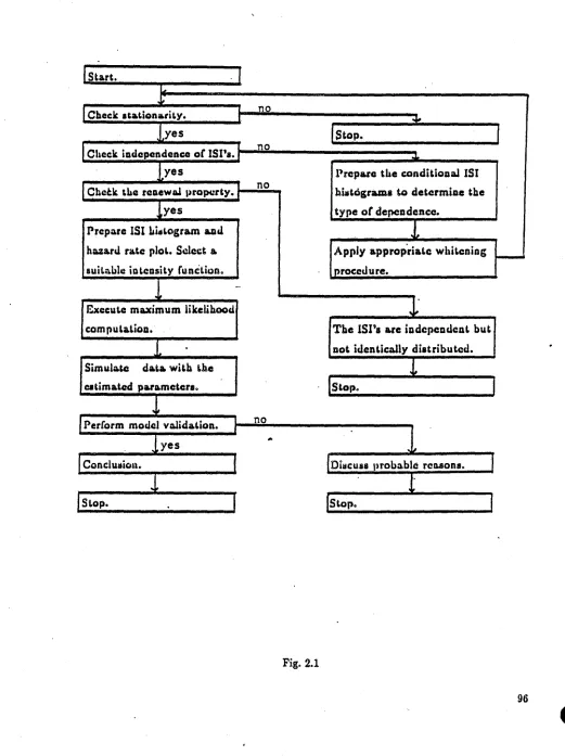
The procedures are put together as a flow-chart in Fig. 2.1. The steps are briefly described as follows:

spontaneous spike-trains and maintained responses of auditory-nerve fibers (see Kiang et al., 1965).

Step I. Check independence among lSI's. The correlogram is a useful tool for this purpose. The

conditional mean plot is also helpful. If the spike-train shows evidence of autCH:orrelation, move toStep.tA.

Step IA. Use the conditional interval histograms to determine the typeofdependence in the lSI's.

When the difference in the conditional interval histograms can be explained solely by the locations of the conditioning intervals, Le., the difference is no more than a shift in the horizontalaxis, a "whitening" procedure somewhat analogous to an AR(1) time series model is

used and the transformed ("whitened") spike-train is sent back to Step 1 again. Details are

illustrated in Section 2.4.

Step 9. Test for the renewal property of the spike-train. The periodogram test (see Cox and Lewis, 1966), or Bartlett's Kolmogorov-Smimov test (see Fuller, 1976), is employed together with conditional interval histograms (see Section 2.3). One possible way for an independent point process to be non-renewal is that it is a semi-alternating renewal (SAR) point process

(Kwaadsteniet, 1982).

Step

4.

Select an intensity function and carry out maximum likelihood estimation.

Step 5. Use the estimates of the parameters to simulate data to be compared with the original spike-train. For the non-renewal case, generate renewal data using the parameter estimates, and then reverse the whitening procedure. Finally, compare this resultant spike-train with the original spike-train before whitening.

The data sets used in this chapter: NERVE1 and NERVE2 are generated using the afterhyperpolarization model given by Smith and Goldberg, 1986. The data set LS7712 was simulated using Exercise 7.7.12

hi

Larson and Shubert, 1979. Each of them contains 2000 interspike intervals. All of them pass Step 1above. The Wald-Wolfowitz runs test statistics for them are .0323, 0.7641, and 0.8701, respectively. That is, they all pass this stationarity test since the test statistics should be asymptotically normally distributed with mean 0 and variance 1

under the null hypothesis. As we will see in the next section, the firing rate plots of them (Figs. 2.2, 2.5, and 2.10) did not show any trend.

So far, we have done Step 1 for allthree spike-trains. Before going into other diagnostic steps, the graphical tools used throughout this thesis for diagnostic steps will be described explicitly in the next section.

2.3 ThegraphiGlIdiagnostictools

The principal graphical tools used in this thesis are derived from the conditional interval histograms. Conditional interval histograms are plotted as follows: group the pairs of interspike intervals (ric-i'

r,J

into 20 equal cell size groups according to the magnitude of the conditioning interval, i.e., the fmt one ineach

Pair,

then plot the histogram ofthe latter one for each group. The integer ; denotes the order of the conditioning, with 1 being the one most frequently used. Each histogram represents 5% of the total number of observations. If the spike-train is renewal, then the conditional interval histograms will be identical to within sampling error. In the non-renewal case, the conditional interval histograms can differ in a number of ways.

The conditional interval histograms of a particular data set are arranged such that the histogram with the smallest conditioning interval is at the upper left comer. The one with second smallest conditioning interval is just below it. The histogram with the largest conditioning interval is in the lower right comer. The conditional interval histograms of NERVE1 are numbered from 1 to 20 and shown in Fig. 2.3 to illustrate the increasing direction of the magnitudes of the conditioning intervals.

The graphical tool that is used frequently in this thesis is the combination of eight plots. The combination is called the 'conditional plots' for convenience. On each page of the conditional plots, there are: the firing rate plot,the serial correlogram, the conditional mean plot, the conditional quantiles plot, the conditional standard deviation plot, the conditional coefficient of variation (CV) plot, residuals of conditional means plot, and Pearson plot. There is a correspondence between the conditional interval histograms and the conditional mean, quantiles, standard deviation, and CV plots. Each point (or set of points, as in the conditional quantiles plot) of the conditional plots just mentioned correspond to one histogram out of the 20 conditional interval histograms. The horizontal ~oordinates of the conditional mean,' quantiles, standard deviation, and CV plots are the magnitudes of the conditioning intervals which are the same as the set of conditioning intervals in the conditional interval histograms. Said another way,

the conditional interval histograms are summarized with the four conditional plots mentioned above. Some of the points in the demo plots shown in Fig. 2.2 for NERVEI are numbered to illustrate their correspondence with the conditional interval histograms shown in Fig. 2.3.

These eight plots as they appear in the diagram below were put together to provide information about a given spike-train. Only the :first three, the firing rate plot, the serial conelogram, and the conditional mean plot are interpreted and made use of explicitly in this chapter, the others are all for later reference. The construction of these plots, using Fig. 2.2 asan example, are describedasfollows:.

(a) Firing rate plot

40 windows of approximately equal length are taken along the time of observation of the spike-train. The average firi~g rate (number of spikes/window length) in terms of number of spikes per second in each window coverage is calculated and plotted against its window number. This is to detect systematic changes in firing rates. The overall firing rate of the entire spike-train is also plottedasa reference line. The firing rate plots ofNERVEI (Fig. 2.2), NERVE2 (Fig. 2.5), and LS7712 (Fig. 2.10) did not show any obvious trend.

(b) Serial conelogram

The Pearson's correlation coefficients up to lag 24 are plotted against their lags. The

upper and lower limits of the asymptotic individual 95% confidence interval, and the horizontal reference line of zero correlation are plotted to show whether a correlation coefficient is significant. There is no significant correlation of any order in NERVE1 (Fig. 2.2). The first order correlation coefficients of NERVE2 and LS7712 are significantly negative (Figs. 2.5 and 2.10).

(c) Conditional mean plot

The pairs (1'"._1' 'T.) of the interspike intervals {'Tn: n~ l} are grouped with respect to the magnitude of the conditioning interval 'T.-1into 20equal cell size bins corresponding to 5% quantiles. The mean of the conditioned interval'T. is plottedag~t the midpoint of the interval in which its conditioning interval falls. The ordinate of each point represents the mean of the corresponding conditional interval histogram. Some of the points are numbered to show the correspondence with the conditional interval histograms shown in Fig. 2.3.

Incalculating the measure for correlations, a linear regression was run on the conditional means without the first and the last points. The slope and its standard error estimates were included in the title of the plot. A linear approximation based on the linear regression and the overall mean are plotted with the conditional means. There is no significant trend in the conditional mean plot of NERVE1 (Fig. 2.2). The negative trend in the conditional mean plots of NERVE2 and LS7712 (Figs. 2.5, 2.10) are all significant.

(d) Conditional quantiles plot

Binning the conditioning intervals in the same way as in the conditional mean plot, the 5%, 25%, 50%, 75%, and 95% percentiles of the groups of the conditioned intervals 'T. are plotted against the midpoints of the intervals in which the conditioning intervals 'T. fall. Parallel conditional quantiles implies the grouped samples are either identical or at most subject to a location shift. More detailed discussions are in Chapter 3. Each set of 5 points that fall on the ,same vertical line represent the 5%, 25%, 50%, 75%, and 95% percentiles of the corresponding conditional interval histograms. Some points are numbered for matching the conditional interval histograms.

The conditional quantiles of NERVE1 as shown in Fig. 2.2 are parallel and flat. The conditional quantiles shown in Fig. 2.5 for NERVE2 are parallel but there is a negative slope. The conditional quantiles of L57712 as shown in Fig. 2.10 spread out with non-positive slopes. The results show that !"fERVE1 may be independent while NERVE2 and L57712 are not.

(e) Conditional standard deviation plot

conditioning interval. This is an indicator of the spread of the conditional distributions. The overall standard deviation is plotted as a line along withth~ con~itionalones. NERVE1.does not show significant change in its conditional standard deviation plot. A more detailed description is

alsoin Chapter 3.

The conditional standard deviation plots of NERVE1 (Fig. 2.2) and NERVE2 (Fig. 2.5) are constant. The conditional standard deviation of L87712 is decreasing (Fig. 2.10).

(f) Conditional coefficient variation (CV) plot

The coefficient of variation of each conditional group is now plotted against its conditioning interval. The overall CV is alsoplotted for reference. The behavior of the conditional CV of a gamma distribution is discussed in Chapter 3. Here NERVE1 did not show an obvious change in its conditional CV plot.

The conditional CV of NERVE1 is approximately constant (Fig. 2.2). The conditional CV plots of NERVE2 (Fig. 2.5) and L87712 (Fig. 2.10) are increasing.

(g) Residual of conditional mean plot

This is the residual plot of (c) to check whether thefit is adequate. A random scattering can conclude the adequacy of the linear fitting. NERVE1 (Fig. 2.2) and NERVE2 (Fig. 2.5) displayed a typical random scattering in its residuals. The residuals of the conditional mean plot of L87712 (Fig. 2.10) displayed a pattern that suggests an increasing variation, which matches its conditional quantiles plot.

(h) Pearson plot

The plot of the moments of the conditional groups is used to confirm that the conditional distribution is not too far away from gamma. This is used as a supplementary tool which is not emphasized in this chapter. Two reference lines are plotted, the line with higher slope is for inverse Gaussian distribution, and the other is for gamma (Correia and Landolt, 1977, Lanskyet aI., 1989). The reference line for gamma distribution is

excess=j. skewnesil,

and the one for inverse Gaussian is

where excess={J2 - 3and skewness=.jP;.

This plot for NERVE1 suggests that the conditional interval histograms may be close to gamma. The Pearson plot of NERVE2 (Fig. 2.5) says that the conditional interval distribution may not be close to a gamma distribution. The plot for LS7712 (Fig. 2.10) says that LS7712 is far from being gamma which will be seen in Section 2.6.

The difference of the conditional plots in Chapter 3 from the one used.elsewhere in this thesis is in the plot labeled (g). Thisis the plot of conditional skewness against its conditional CV (e.g., Fig. 3.1). As in the Pearson plot, this is used. as a diagnostic tool for confirming whether a sample is from a gamma distribution. Two reference lines were plotted with the points. The upper one for inverse Gaussian is defined as

.kewness=3·CV.

and the lower one for gamma is defined as

.kewnes.=2·CV

(Kendall and Stuart, 1977).

2.4 TheRenewal e-NERVEI

NERVE1 passes. Step 1 as stated in Section 2.2. The correlogram and the conditional mean plot do not show any significant dependence in the interspike intervals of NERVE1 as shown in the conditional plots as shown in Fig: 2.2. Then the test statistic of NERVE1 for the periodogram test is 0.0174, which suggests that NERVE1 is renewal. The conditional interval histograms of NERVE1, as shown in Fig. 2.3, further support th,at NERVE1 is renewal since there is no significant difference among the histograms. NERVE1 can then be treated as a stationary renewal process. The next step is to select an intensity function and carry out the maximum likelihood estimation procedure.

The selected intensity function is

It is seen that the model contains a constant signal rate~, a recovery shape constant 0',

a recovery time constant

p,

and the recovery function r(.), as seen in Section 2.1, exponentially approaches 1. The likelihood equations and the maximum log-likelihoods (m.l.l.) ofthismodel are derived without the dead-time ttl and are derived in Appendix A.

A similar intensity model can be found in Gaumound et al., 1982 with 0'=0.5.

The deadtime ttl is considered fIXed in this model. The maximum likelihood estimation is basically a three dimensional grid search. For each fixed dead-time, the likelihood equation

•

defines a smooth surface in the space spanned by ~, &, and '/3, and hence a surface in the parameter space.It is difficult to illustrate this surface in the parameter space spanned by ~, 0',

p,

and ttl. The numbers listed in Table 2.1 should help to visualize how the log-likelihood function varies as each of the parameters changes. The maximum likelihood estimates are

~=0.1996,&=2.50, '/3=7.0, and

t,,=1.87.

The spike-train simulated using the maximum likelihood estimates is compared with NERVE1- The main evidence validating the model is the Kolmogorov-Smimov two sample test result. The test statistic is 1.1068, and the p-value is 0.1641. This test is meaningful here since the spike-train is renewal. The estimated intensity function is plotted over the empirical hazard rate (Fig. 2.4) to illustrate the degree of fit. The measures for skewness for the original and the reproduced spike-train are 2.175 and 1.522, respectively. The measures for kurtosis for the original and the reproduced spike-trains are 9.478 and 3.779, respectively. The maximum interval for the original NERVE1 is 63.6 ms. while the maximum interval for the reproduced spike-train is only 48.5. These imply that the estimated intensity function may not reproduce the behavior in the tail well enough.

2.5TheNon-renewal Use-NERVE2

NERVE2 passes Step 1 as shown in Section 2.2. The correlogram and the conditional mean plot suggest that there is a negative serial dependence (Fig. 2.5). The periodogram test is

performed on NERVE2 to confirm that the renewal hypothesis is rejected at the 0.01 level of significance as expected. We then move to Step RAfor the "whitening" procedure for NERVE2.

/

There is a special class of spike-trains that produce conditional interval histograms differing only in the location but notin shape (see Johnson et al., 1986). It is expected that once the current interval is adjusted for the shifting effect contributed by ita conditioning interval, then the resultant new spike-train will be free of the type of dependence that usedto exist between the adjacent intervals of the interspike intervals of the original spike-train. This is exactly what a whitening procedure does and creates a whitened spike-train { Tn; n~I} that is 'renewal. One way to determine the effect of the conditioning interval is by computing the conditional expectation of the k-thinterspike interval given the(k - ;)-th_, interspike interval. That is,

E[ 151"

I

r,,_J

=

C·,(ric_V

where C is a positive constant. The resultant (whitened) spike-train {r'n; n~I} is defined to be

{ h[rn-,(rn-Vl; n~I},

for some function h(.). This implies that the conditional mean plot in Step

t,

or some plots equivalent to it, can be used to fmd the function ,(.) within a certain range. If ,(r

n-V

is nonconstant for some ;>1, i.e., higher than first order dependence, then these expectations should be redone, simultaneous conditioning on the; previous intervals. This produces a multivariate form for ,(. ) and hence requires larger data sets. For our example, only first order dependence was indicated.

The correlogram of NERVE2 in Fig. 2.5 shows that first order correlation is the only significant one, and the conditional mean plot in Fig. 2.5 shows a nearly linear pattern. The conditional interval histograms in Fig. 2.6 show that nothing more than a shift is observed among the histograms. That is, the above whitening procedure seems appropriate here. In determining the functional form ,(.) mentioned above, a simple linear function inric-I is considered because the conditional mean plot is almost perfectly linear. The ordinary linear regression on all except the first and the last points gave a slope estimate of - 0.1561 (0.0241). That is

E[ ISln

I

rn-l1

=-

0.1561 •rn-l

+

C.

So the whitened spike-train is defined as

{ Tn

+

0.1561 • rn-l; n~1}.

The reason for excluding the two end points isth~t the first and the last 5% quantiles tend to be noisy and become outliers in fitting a regression line.

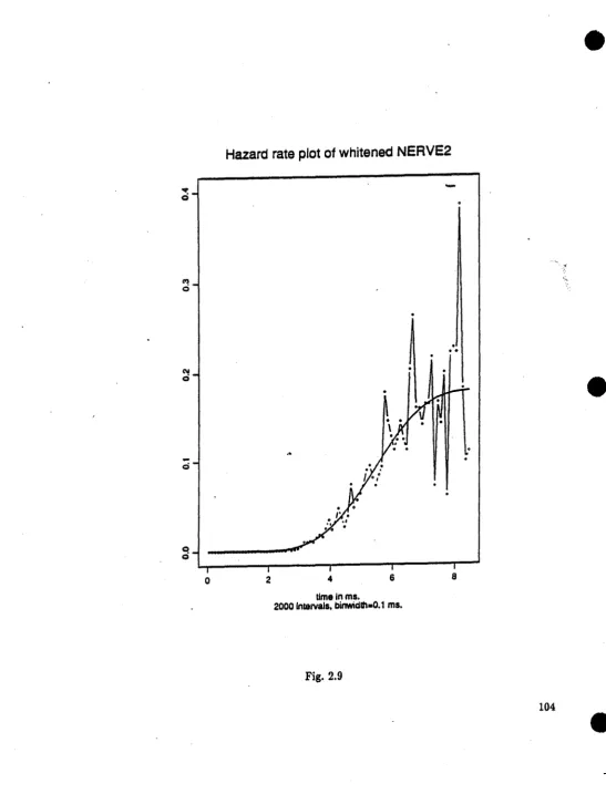
the whitened NERVE2 all support that the whitening is working. The periodogram test statistic of 0.0277 assures· that it is renewal. The whitened spike-train NERVE2 is now ready for maximum likelihood estimation.

The model used here for the whitened NERVE2 is the same as in Section 2.3. The computed estimates are:

td=1.34,

&=3.6,

ft=4.5,

).0=1.7976. The behavior of the likelihood surface is summarized in Table 2.2. The hazard rate plot of the whitened NERVE2 with the estimated intensity curve is shown in Fig. 2.9 to illustrate the fit.

AB for the verification of the identity of two non-renewal spike-trains, there is not a generally established criterion. One way to do it is to combine the results of the comparisons between the two sets of conditional interval histograms and the significant correlation coefficients of the two target spike-trains. Since the non-renewal spike-train, NERVE2, was assumed to have a fairly simple correlation structure, the criteria emphasize only the first order correlation rather than~general joint distribution point of view (c.f. Cox and Isham, 1980).

2.6 An analytical exampl.LSll12

The type of correlation of LS7712 as illustrated in its conditional plots (Fig. 2.10) is, although unknown, different from that in NERVE2. The greatest difference is that the conditional distributions are spreading out as the conditioning interval increases. Before any statistical properties can be determined, it was examined how LS7712 was generated.

The 2000 interspike intervals of LS7712 {Tn;n=I,2, ...,2000} were simulated as follows:

T 1 - Uniform(O,I),

and

Tn+1

I

Tn - Uniform(1 - Tn' 1).

Itcanbe seen that the distribution ofTn

+

1is conditioned on the realization of its predecessorrn' It was shown by that LS7712 passedthe Wald-'Voolfowitz runs test for stationarity, soLS7712 is considered to be non-renewal but stationary.

intervals lie in the range from 0 to 1MS. This is highly unlikely in the real world but analysis will

be done as is. Also, there is a limit of accuracy of the spike recording device in the laboratory, usually up to 10 micro-seconds, i.e., 0.01 milli-second (ma.). But in LS7712, no such limit was assumed and there were eight digits after the decimal point in each interspike interval. We will imagine a suitable time unit for LS7712 and this should have no effect on the procedures done to it.

Since the generating mechanism of LS7712 is completely specified, we can start with the finite dimensional joint distribution of its interspike intervals. LS7712 is a realization of a Markov process since

where '_{R (· )} is an indicator function such that

1, i(xE R

0, i(x¢ R.

This reduces the consideration of joint distributions to bivariate joint distributions.

It is clear that

E{

rn

+

1

I.,.,J=1 - 0.5·

rn'

vat(l'n

+

1

I.,.

nJ=r~12.

So

=1 - 0.5 •Ern

_lEr

n

_ir

n-1

I

r

n -

J]

=1- 0.5+ 0.52-0.s1- ...+(- 0.5yn-2+( - 0.5r-1•

Er/rJ

=1- 0.5+ 0.52- 0.s1- ...

+ (-

0.5yn-2

+ (-

0.5yn-l. 0.5

-. 2/3 asn-+00.

Since

then

-. 0.5 asn-+oo.

Hence

VIIr(r,J-+ 0.5 - (2/3'=1/18 asn-+oo.

f,(y)= / : fYIX(Ylx) • f,(x)dx.

exists only for a stationary Markov process. Therefore if there exists a unique solution f,for the equation

for n~1, then it can be said that L87712 is a realization of a stationary Markov process. It is found that

since the support of the stationary distribution, if it exists, will be the interval (0,1). Therefore it canbeassumed that .

Then the equation becomes

=/00 (l/rrJ . g.(rrJ

"(O,l)(rrJ •

'(l-r ,1)(r

n

+

1

)drn

o n

=/1

(l/rrJ . g'(rrJdr

n .

'(o,llr

n+l)'

1-r

n

+

1

Thus

Itis straight-forward that

that is,

.'.(X)=2'X·'(O,I)fX)

is the stationary distribution of the interspike intervals of LS7712. The mean and variance are 2/3 and 1/18, respectively.

It has been shown that LS7712 has a stationary distribution. But the distribution ofr1is

not the same. Hence LS7712 is a homogeneous but non-stationary Markov process. The Wald-Wolfowitz runs test shows that the evidence is not strong enough to conclude that LS7712 is not stationary. Since we are dealing with only one realization of a Markov process, it would not make a great difference how the initial value was generated, especially when the difference in the distributions is not great. LS7712 willbetreated asifit is stationary.

To further confirm the stationary distribution and that ~)le departure of LS7712 from being stationary is sufficiently small, a Kolmogorov-Smirnov test ofgQ.odness-of-fit gives a p-value of 0.827, saying that there is not enough evidence to conclude that the marginal distribution of the interspike intervals from LS7712 is different from its stationary distribution. The skewness of LS7712 and the stationary distribution were calculated to be-0.007896 and -0.00741, respectively. The difference is small. The interval histogram of LS7712 (Fig. 2.12) has a triangular shape coinciding with the shape of its stationary distribution.

The same diagnostic steps as those performed on NERVE1 and NERVE2 give evidence that LS7712 is not renewal. The first-order correlation coefficient is significantly negative

(PI= - 0.4839). The conditional mean plot (Fig.2.10) gives a significant negative slope ( - 0.4776 (0.0268» which is close to its theoretical value - 0.5. The significant periodogram test result (0.3250 vs. .05-level critical value 0.0430) and the conditional interval histograms (Fig. 2.11) show also that LS7712 is not renewal. A whitening procedure, if one exists, is necessary for LS7712 tobefurther analyzed.

The first try is to use the same AR(l) analog method as for NERVE2 since the linear trend in the conditional mean plot of LS7712 issoobvious. That is, we take