Predicting attack-prone components

Predicting Attack-prone Components

1

Michael Gegick,

Pete Rotella and

Laurie Williams

North Carolina State University Department of Computer Science,

Cisco Systems, Inc.

{mcgegick, lawilli3}@ncsu.edu, [email protected]

Abstract

Limited resources preclude software engineers from finding and fixing all vulnerabilities in a software system. This limitation necessitates security risk management where security efforts are prioritized to the highest risk vulnerabilities that cause the most damage to the end user. We created a predictive model that identifies the software components that pose the highest security risk in order to prioritize security fortification efforts. The input variables to our model are available early in the software life cycle and include security-related static analysis tool warnings, code churn and size, and faults identified by manual inspections. These metrics are validated against vulnerabilities reported by testing and those found in the field. We evaluated our model on a large Cisco software system and found that 75.6% of the system's vulnerable components are in the top 18.6% of the components predicted to be vulnerable. The model’s false positive rate is 47.4% of this top 18.6% or 9.1% of the total system components. We quantified the goodness of fit of our model to the Cisco data set using a receiver operating characteristic curve that shows 94.4% of the area is under the curve.

1. Introduction

Security vulnerabilities can occur because of subtleties and false assumptions in the design or code of a software system [20]. Security engineers need more time to uncover and fix these problems than their release schedule permits, and so vulnerabilities are inevitably released with the software. Compounding this schedule problem is that there are usually far fewer security engineers assigned to projects than general reliability engineers, but are responsible for testing the security posture of the entire system. Also, attackers have the advantage of time, in that they can spend months or years building an exploit for just one area of the software system. Collectively, these conditions

necessitate security risk management where security efforts are prioritized to the highest security risk software components1 _{to minimize damage to the end} user.

In addition to prioritizing which components to fix, it is also important to fix the components early. The costs to fix faults in the testing phase can be nine times cheaper than fixing during operation [2]. An early knowledge of which components should receive the most security effort can also reduce the number of end-user-installed security patches.

The objective of this research is to create and evaluate models that predict which components are most susceptible to attack. The results of the models are available early (i.e. before system-level testing begins) in the software life cycle (SLC) allowing recovery time for inspections, re-design, and test efforts for the most vulnerable software components.

The input variables to our model include security-related static analysis tool warnings, code size and churn, and all faults identified by manual inspections. These metrics are validated, using classification and regression trees (CART), against vulnerabilities reported by testing failures and those found in the field. We evaluated our model on a large Cisco software system to determine the model’s efficacy. We also developed a cost model for our predictive model that provides estimates of costs to remediate vulnerable components. During our empirical case study, we developed a sequential tree method to refine our models. We describe our experience and findings on how to lower false negative rates associated with our predictive models.

In Section 2 we provide background and related work; in Section 3 we explain our empirical case study; in Section 4 we present our research methodology; in Section 5 we describe the threats to the validity of our approach; in Section 6 we discuss results; in Section 7 we outline our sequential tree approach; and we summarize in Section 8.

1 _{A component is one of the parts that make up a software}

2. Background and related work

2.1. Vulnerability prediction models

Neuhaus et al. [25] have investigated predictive models that identify vulnerability-prone components. They created a software tool, Vulture, that mines a bug database for data including libraries and APIs to identify vulnerable components. They performed an analysis with Vulture on Bugzilla, the bug database for the Mozilla browser, using imports and function calls as predictors. They identified 45% of all of the vulnerable components in Mozilla with a 30% false positive rate.

In an earlier case study involving a large telecommunications system [10], we used a CART model to assign a probability of attack to each file. Upon ranking these probabilities in descending order, we found that 72% of the attack-prone files are in the top 10% of the ranked files and 90% are in the top 20% of the files. The input variables for that study consisted of the count of Klocwork2 _{static analysis tool} warnings, a measure of file coupling (a complexity metric), and the count of added and changed source lines of code. In our other earlier work [11], we used CART to predict which components were attack-prone using warnings from the FlexeLint3 _{static analysis tool,} and code churn. The model identified all of the attack-prone components, but with an 8% false positive rate. Ozment and Schechter [27] did not find a significant correlation between code churn and vulnerability count, but their correlations were performed at the version level of OpenBSD, while our study was performed at the file level. The study in this paper is based on a different software technology and from a different vendor than in our earlier studies.

2.2. Automated static analysis (ASA)

We use static analysis tool output as one of our candidate metrics for the case study in this paper. A static analysis tool analyzes the content of a software system to detect faults without executing the code [4]. We use the term “automated static analysis” (ASA) to refer to the use of static analysis tools. Examples of the types of problems identified by ASA tools include the detection of calls to potentially insecure library functions, bounds-checking errors and scalar type confusion. ASA tools perform analyses such as semantic, structural, configuration, control- and data-flow analyses. The output of an ASA tool is a

2 _{http://www.klocwork.com}

3 _{http://www.gimpel.com}

warning. The warnings describe a fault in the software that could lead to a failure. A true positive is a warning that describes a fault that can cause a failure, and a false positive is a warning that misclassifies code as faulty. Increasingly, ASA tools are used to identify security vulnerabilities [5].

Recently, models classified prone and not fault-prone components using ASA warnings as input variables for discriminant analysis [23]. Nagappan et al. [23] demonstrated that they could distinguish 82.91% of their fault-prone components. Their results indicate that a separation can be made between fault-prone and not fault-fault-prone components to confidently prioritize the allocation of testing resources and inspections. Zheng et al. [32] correctly classified 87.5% of the modules in their study when the number of ASA faults and number of test failures are considered. Their work is based on the idea that one technique (e.g., ASA) alone is insufficient for finding all faults in software [31], but that coding problems reside in the same locations as bigger problems identified by testing. Our research tests whether or not vulnerabilities identified by ASA are a bellwether of other types (e.g., design-level) of vulnerabilities.

2.3. Statistical overview

The input variables, data set, distribution (e.g., Poisson), and the statistical technique (e.g. multiple linear regression) constitute a statistical model [19].

2.3.1. Correlations and collinearity

A correlation coefficient, r, measures how strongly two variables are related [6]. A correlation coefficient has a value between -1 and 1, inclusive. A weak correlation has a value between 0 and 0.5 and a strong correlation is greater than or equal to 0.8, otherwise the correlation is moderate [6]. Collinearity is defined as a high degree of correlation between the independent variables of a statistical model [8]. Collinearity occurs when an excessive number of input variables are used to determine an outcome, and the input variables measure the same outcome [8].

2.3.2. Cross-validation and ROC curves

approximately equal numbers of randomly chosen components. One group is used as the test set and the training set consists of the remaining four groups of components. The model is trained on the training set, and the training analysis is compared to the outcomes of the test set to validate how well the model performs on data that has not been “seen” before. Each of the five groups of components takes one turn as the test set, so five analyses are required. After the five analyses are performed, the average error is calculated over the five trials.

We will use receiver operating characteristic (ROC) curves to quantify the goodness of fit of the model to the data set. The y-axis of the ROC curve is the true positive rate of the predictive model and the x-axis is the false positive rate.

2.3.3. Classification and regression trees (CART)

CART is a statistical technique that recursively partitions data according to X and Y values. The result of partitioning is a tree of groups where the X values of each group best predicts a Y value. The leaves of the tree are determined by the largest likelihood-ratio chi-square statistic. The threshold, or split, between leaves is chosen by maximizing the difference in the responses between any two leaves [28]. For the case study reported in this paper, the X values are the candidate metrics and the Y value is a binary value describing a component as attack-prone (value of one) or not attack-prone (value of zero). The CART technique has been shown to be useful for distinguishing failure-prone from not failure-prone components in the reliability realm [29].

3. Cisco empirical case study

We performed an empirical case study on a Cisco software system that was implemented in the C programming language. The system is divided into well-defined components upon which our analyses are based. At Cisco, a component is a unit of a software system that typically consists of ten or more files. The count of components is large enough to perform rigorous statistical analyses. We do not provide details of this system due to the proprietary nature of the data. Our goal is to determine if early (pre-system-level testing) metrics predict which components will have security failures found late (during system-level testing and in the field) in the SLC.

3.1. Candidate metrics

We strategically chose five metrics for our predictive models so our analyses can be easily repeated and adopted by software engineers. Good

metrics are those where measurements of the software are objective, reproducible, and empirical [15]. For example, a software engineer can use a tool to objectively measure source lines of code (SLOC) in a file in order to provide the count of SLOC as a metric for an analysis. The measurements that provide the metrics should also be performed easily and economically [15]. Additionally, we required the metrics to be accessible early in the SLC to afford software engineers a means to prioritize security efforts during development. We now discuss our candidate metrics that will serve as the input variables for our predictive model.

The first metric is the count and density of warnings produced by two ASA tools that will be called Tool 1 and Tool 2. The names of the tools are not revealed, but these tools are widely used tools in the industry. Cisco requires that ASA be performed on all components, and validating this metric as a vulnerability predictor can potentially aid security efforts for all Cisco software. We focus on the security-related ASA warnings from Tool 1 to determine if security warnings alone are better predictors of security vulnerabilities than non-security warnings. Examples of Tool 1’s security warnings are buffer overflows, poor encryption, permissions problems, and race conditions. We also include null dereferences and memory leaks, which have been documented as causing security problems [21].

We do not restrict our metrics to the security realm, however. Our prior work [9, 12, 13] indicates that non-security failures are positively correlated with security failures, and we therefore do not exclude non-security warnings as candidate metrics. We include non-security warnings from Tool 2, for example, that include suspicious use of semicolons and ignoring return values of functions.

The ASA warnings in our case study unavoidably include both true positives and false positives. If the false positives from the ASA have predictive power in our models, then a time-intensive audit for removing false positives is not required to predict vulnerabilities. By including false positives, we abide by our candidate metric selection criterion that requires that measurements be easily performed.

own the code, but they have not interacted with the code for a length of time, then they may not be familiar with the underlying assumptions of how that code operates. A vulnerability can be injected into the code when assumptions are made during the code change that are not consistent with the underlying code’s assumptions. McGraw [20] uses ambiguity analyses to identify inconsistent assumptions to root out vulnerabilities [20]. Additionally, Nagappan et al. [24] have found that code churn is a predictor of fault-prone components.

Our third metric is the count of SLOC, which is measured in thousands of SLOC (KSLOC), and can be obtained when calculating code churn. We will test if larger software components are more vulnerable.

The fourth and fifth candidate metrics are the count of faults reported by pre-testing manual static inspections and failures identified by unit testing. The static inspections include faults identified during design reviews and code reviews. These metrics may indicate that faults found early in the SLC are an indicator of faults found later in the SLC. The faults identified by static inspections and unit tests are easily obtainable via queries to the Cisco fault database and are thus included as metrics for our case study.

We suspect that as the values of these five metrics grow in a component then so will the count of vulnerabilities.

3.2. Security vulnerabilities

The Cisco Security Evaluation Office (SEO) provided us with the security failures for our case study. The SEO tracks vulnerability trends at Cisco and is thus an optimal source for security data. Software engineers identified these security failures during the testing phase, which includes security testing, stress testing, system testing, and feature/function-level testing. The SEO also provided security failures identified during internal usage and those reported by customers and third-party researchers. These security failures comprise the dependent variable for our predictive models, and will be used to validate if the afore mentioned candidate metrics are good predictors of these security failures. The count and types of security failure reports4 _{are not} disclosed for confidentiality reasons.

In our setting, an attack-prone component is a component that contains at least one security failure that was identified by testers, customers, or third-party researchers. We use the term “attack-prone” because the security faults were identified during system

4 _{The security data have been slightly and consistently}

modified for confidentiality reasons.

execution. In the context of testing, if a tester discovers a buffer overflow during runtime, we say they have attacked the system. Although the tester may not have exploited the buffer overflow to cause a denial-of-service or to inject code that escalates their privileges, the failure is a proof of concept that the system can be attacked. We use the threshold of one security failure to deem a component attack-prone because there is little variability in the security failure count per component and only one attack is needed to cause substantial business loss. A component with no reported security failures will be called a “not attack-prone” component.

4. Research methodology

Our predictive models5 _{use the candidate metrics to} distinguish between attack-prone and not attack-prone components. During model construction, we maximize the predictive model’s accuracy, but with a small number of included metrics. A larger number of metrics increases the model’s complexity and reduces the likelihood that Cisco software engineers will adopt the model because more time would be required to gather the metrics, build the model, and incorporate its use in the standard workflow.

The metrics in our predictive models can also be called independent variables or input variables. The dependent variable is the count of vulnerabilities in each component, and this count is used for correlation analyses. In the context of classifying components, attack-prone and not attack-prone are the two response levels. These response levels do not indicate the type or count of vulnerabilities; they only represent if a component is associated with at least one reported vulnerability or not. The models may be useful for predicting which components contain vulnerabilities, where the nature of the vulnerability ranges from abstract design vulnerabilities to relatively simple coding vulnerabilities, such as simple buffer overflows.

4.1. Correlations to vulnerabilities

We will first test if the candidate metrics are correlated with the count of vulnerabilities identified during testing, internal use, and by customers. When the metrics are significantly correlated with vulnerabilities, they are good candidates for the predictive models. During candidate metric selection, we also test the metrics for collinearity. If the metrics are correlated with each other, we have to simplify the model or perform additional analyses to reduce the collinearity.

4.2. Discriminatory techniques

We use the following three statistical discriminatory techniques in our models: Discriminant analysis, logistic regression, and CART. Each technique classifies observations into distinct groups. These techniques have been shown to be successful in classifying fault-prone and not fault-prone modules in the reliability realm [18]. In our setting, we use a dichotomized scheme where components are labeled attack-prone or not attack-prone according to the approach outlined in Section 3.2.

The execution of these three statistical techniques examines different combinations, counts, and orders of metrics entered into the model. A good combination of metrics in the model both separates attack-prone and not attack-prone components and maximizes the R2 value of each model. R2 is a measure of the variance in the data that is explained by the model [22].

In the CART technique, each leaf of the tree contains a subset of the system components. A single leaf in the CART tree can then be split further into two leaves by including a metric to increase the probability that one leaf will likely contain attack-prone components while the other leaf will not likely contain attack-prone components. During our CART analysis, each leaf is split into two leaves if and only if the p-value is at or below 0.05. If the p-value is above 0.05, then we are less confident that the groups of components in the two leaves are sufficiently different to warrant the use of separate leaves.

4.3. Model validation

A ROC curve that has less than 50% of the area under the curve will be rejected, since the model will not have demonstrated a good fit to the Cisco data set. Additionally, the models are cross-validated to determine if the R2 of the overall model is consistent with the R2 of the cross-validated model. If the R2 values are consistent, then the variation explained by the predictive model is an accurate description of the model performance. A model with a higher R2 explains more variance than a model with a low R2.

4.4. Hypotheses

The null (H0) and alternative (HA) hypotheses are stated here. If the predictive model can distinguish attack-prone from not attack-prone components with statistical significance, then we do not reject HA.

H0: The candidate metrics have no predictive power in a statistical model that indicates which components contain vulnerabilities identified during testing, internal use, and customer use.

HA: The candidate metrics do have predictive power in a statistical model that indicates which components contain vulnerabilities identified during testing, internal use, and customer use.

4.5. Model efficacy

The models’ efficacies are reported in terms of Type I (false positive) and Type II (false negative) error rates. Also, we will provide precision, accuracy, and recall values. The techniques that yield the lowest Type I and Type II error rates are then selected for the predictive models. These terms are now defined.

True positive (TP) – a component correctly classified as attack-prone by the model.

False positive (FP) – a component misclassified as attack-prone by the model.

False negative (FN) – a component misclassified as not attack-prone by the model.

True negative (TN) – a component correctly classified as not attack-prone by the model.

We give measures of accuracy to indicate the overall success of the model; measure of precision to indicate how many not attack-prone components are false positives; and measures of recall to indicate how well the model correctly classifies attack-prone components.

Accuracy - (TP + TN)/(TP + FP + TN + FN)

Precision - (TP)/(TP+FP)

Recall - (TP)/(TP+FN)

5. Threats to validity

Software faults identified by testing failures do not represent the entire set of faults in the software system [7], and we cannot be certain that all components have been inspected and tested equally. Additionally, the customer-reported failures do not completely identify all security faults latent in the system. Also, developers and testers may not have recognized all faults that are security-related and thus did not submit them to the SEO. As a result of these uncertainties, our analyses are necessarily based on incomplete data. Adding to this, security issues are rare events in software systems [1]. The scarcity of data makes statistical analyses difficult. For example, the Spearman rank correlation may not perform optimally in zero-inflated data that represent components with no reported security problems. Lastly, the models presented in this paper are representative of one industrial software system, and will not necessarily

6. Results

We now report the results of our method. All analyses are on a per component basis.

6.1. Correlation to vulnerability counts

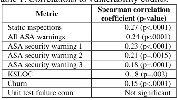
The results of the correlation analysis show that the sum of faults from manual design reviews and code reviews has the highest correlation (0.27) to the vulnerability count, as shown in Table 1. The correlation is weak, but is significant (p<.0001) and therefore is not excluded from our predictive models.

The correlation between all ASA warnings from both tools combined and vulnerability count is 0.24. We do not rule out that a general reliability ASA warning can cause a vulnerability, but we suspect that general reliability warnings, such as “suspicious use of semicolons,” are less likely to be vulnerabilities in software than other ASA warning types. The results indicate that general coding problems detectable by ASA have a nearly identical correlation to vulnerability counts as ASA security warning type 1, as shown in Table 1. The specific ASA security warning types are not revealed here, for confidentiality reasons. The vulnerabilities (i.e., the dependent variable) found by testing, internal use, and the customers are correlated to the population of all ASA warnings, and this indicates that where there are known coding problems there may be more complex security problems, too.

Table 1. Correlations to vulnerability counts.

Metric Spearman correlation coefficient (p-value) Static inspections 0.27 (p<.0001) All ASA warnings 0.24 (p<0001) ASA security warning 1 0.23 (p<.0001) ASA security warning 2 0.21 (p=.0015) ASA security warning 3 0.18 (p=.0001) KSLOC 0.18 (p=.002)

Churn 0.15 (p<.0001)

Unit test failure count Not significant

6.2. Tests for collinearity

We tested the collinearity between the different candidate metrics. The largest correlation coefficient is 0.56 and exists between KSLOC and all ASA warnings, as shown in Table 2. These candidate metrics were not used together in the same predictive model because the correlation indicates that they describe approximately the same phenomena in the data set. The other correlation coefficients are weak and were therefore not considered a threat to validity. All correlations in Table 2 have a p-value at or below 0.05 (95% significance level).

Table 2. Correlation matrix for candidate metrics.

Metric ASA

Warnings KSLOC Churn

Static inspections

Unit tests ASA

warnings -- 0.56 0.25 0.40 0.16

KSLOC -- -- 0.52 0.40 0.35

Churn -- -- -- 0.34 0.40

Static

inspections -- -- -- -- 0.38

Unit tests -- -- -- -- --

6.3. Predictive models

All discriminant analysis and logistic regression models that were examined produced higher Type I and Type II error rates than our CART models, so they are not included in this paper. We present three separate CART models to show that there is more than one viable model for our data set. Multiple viable models confirm that successful model building for this data set does not require a serendipitous combination of metrics that have good predictive power.

We observed that the attack-prone components are distributed more to the left leaves of the CART trees than the right leaves. Figure 1 shows the tree for Model 3 and the metrics used in this model. In Table 3, we show the results of selecting all components from the leftmost, that is, leftmost until reaching a leaf that has a Type I error rate that surpasses the true positive rate while keeping the total number of components to analyze less than 20% of the total system components.

In Model 3, the six leftmost leaves contain 75.6% of the known attack-prone components and there is a 47.4% Type I error rate in these leftmost leaves, as shown in Table 3. The Type I error rate is 9.1% of the total system components. These leftmost leaves constitute only 18.6% of the total system components.

Table 3. CART model results for three models.

Model

Percent attack-prone components in the

top x% of the ranking (recall)

Type I error

rate

Type II error

rate

% Type I errors of total system Model 1 48.8% in top 7.9% 20.0% 51.2% 1.6% Model 2 63.4% in top 13.6% 39.5% 36.6% 5.4% Model 3 75.6% in top 18.6% 47.4% 24.4% 9.1%

Figure 1. The CART tree for Model 3. Non-shaded boxes are leaves of the resultant tree.

count of ‘a’ ASA buffer overflow warnings, then the child leaf to the left contains all components with greater than or equal to ‘a’ buffer overflows and the components in the right child contain less than ‘a’ buffer overflow warnings. We observe that in Leaf 1 (see Figure 1), the split indicates that the left child of a parent is associated with fewer ASA security warnings. Therefore, components in this left leaf contain fewer warnings of these types, and another unidentified factor not already in our model is contributing to the vulnerabilities. However in this case, the first three splits of the tree are based on a higher portion of warnings and therefore Leaf 1 contains components with more warnings than the leaves in the right half of the tree suggesting that warnings are still a factor for the attack-prone components in Leaf 1.

The vulnerability distribution among components is heavily skewed according to our models. This behavior, referred to as Pareto’s Law, is also seen in the software reliability realm [3, 26].

We provide a visualization of the efficacy of Model 3 (see Figure 2) which shows the skewed nature of the vulnerability data. The large true negative region shows that most of the system components are not attack-prone components and are correctly classified as not attack-prone by the model. Security fortification efforts are not needed in the large true negative region, therefore overall fortification costs are substantially reduced if security engineers do not target this region.

The accuracy, precision, and recall values for the three models are shown in Table 5. Model 3 performs well because the first six leaves in the tree are attack-prone rich.

TN

FP TP

FN

Figure 2. Visualization of the system by Model 3. TN (True Negatives - correctly classified as not attack-prone) FN (False Negatives- misclassified as not attack-prone) TP (True Positives - correctly classified as attack-prone) FP (False Positives - misclassified as attack-prone)

Table 5. Accuracy, precision, recall for three models.

Model Accuracy Precision Recall

Model 1 92.0% 80.0% 48.8% Model 2 90.0% 60.5% 63.4% Model 3 88.0% 52.5% 75.6%

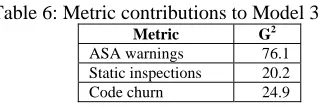
The predictive power of the metrics is measured by the likelihood-ratio chi-square statistic, G2, for each metric. A larger G2 value indicates a better statistical fit, which indicates a better split of the leaves in the CART analysis between prone and not attack-prone components. In Model 3, the total ASA warnings metric contributed the most separation in the overall model, as shown in Table 6. These results show that the faults identifiable by ASA are predictive of different types of security faults that surface during testing and those reported in the field.

Table 6: Metric contributions to Model 3.

Metric G2

ASA warnings 76.1 Static inspections 20.2 Code churn 24.9

Table 4. The CART analysis for Model 3.

Leaf

No. Conditional probability formula

Probability not

attack-prone

Probability

attack-prone

1 SecurityWarningType4>=a&Tool1CountWarnings>=b&Tool2WarningDensity>=c&

SecurityWarningType4Density<d 0.00 1.00

2 SecurityWarningType4>=a&Tool1CountWarnings>=b&Tool2WarningDensity>=c&SecurityWarningT

ype4Density>=d&DesignAnalysisFaults>=e&AllManualStaticInspections<f&SecurityWarningType2>=g 0.00 1.00

3 SecurityWarningType4>=a&Tool1CountWarnings>=b&Tool2WarningDensity>=c&SecurityWarningT

ype4Density>=d&DesignAnalysisFaults>=e&AllManualStaticInspections<f&SecurityWarningType2<g 0.53 0.46 4 SecurityWarningType4>=a&Tool1CountWarnings>=b&Tool2WarningDensity>=c&SecurityWarningT

ype4Density>=d&DesignAnalysisFaults>=e&AllManualStaticInspections>=f 1.00 0.00 5 SecurityWarningType4>=a&Tool1CountWarnings>=b&Tool2WarningDensity>=c&SecurityWarningT

ype4Density>=d&DesignAnalysisFaults<e&SecurityWarningType3<h 0.50 0.50 6 SecurityWarningType4>=a&Tool1CountWarnings>=b&Tool2WarningDensity>=c&SecurityWarningT

ype4Density>=d&DesignAnalysisFaults<e&SecurityWarningType3>=h&Tool2WarningCount>=i 0.62 0.37 7 SecurityWarningType4>=a&Tool1CountWarnings>=b&Tool2WarningDensity>=c&SecurityWarningT

ype4Density>=d&DesignAnalysisFaults<e&SecurityWarningType3>=h&Tool2WarningCount<i 0.98 0.01

8 SecurityWarningType4>=a&Tool1CountWarnings>=b&Tool2WarningDensity<c 1.00 0.00

9 SecurityWarningType4>=a&Tool1CountWarnings<b 0.97 0.02

10 SecurityWarningType4<a&Churn>=j&Churn<k 0.50 0.50

11 SecurityWarningType4<a&Churn>=j&Churn>=k 0.93 0.06

12 SecurityWarningType4<a&Churn<j 1.00 0.00

“…a seemingly worthless split might lead to a very good split below it” [14]. In our earlier study [12], we found that weakly-correlated metrics have discriminatory power equal to strongly-correlated non-security failures. The weaker metrics have less significant splits, although the p-values are below 0.05, than the strongly-correlated metric. However, our observations in [12], and in comparison of the results presented here with those in [13], we find that weakly-correlated metrics can lead to more splits than strongly-correlated metrics, and that many splits can yield good separation between attack-prone and not attack-prone components.

6.4. Model validation

We evaluated the models using ROC curves and five-fold cross-validation. The ROC curve for Model 3 has 94.4% of the area under the curve, indicating that the model demonstrates a good fit to the Cisco data set (see Figure 3). The weighted line is a representation of the sorting efficiency of the estimated probabilities that a component is attack-prone. The diagonal line serves as a baseline, where the false positive rate is equal to the true positive rate. The cross-validated R2 values (see Table 7) indicate that not all variance in the data is accounted for, but the overall R2 values are fairly consistent with the cross-validated R2 values.

Table 7. ROC curve and R2 values for three models.

Model ROC R2 Cross-validated

R2

Model 3 94.4% 55.6% 50.4%

Model 1 94.0% 57.4% 53.7%

Model 2 88.0% 48.0% 42.8%

S

e

n

s

itiv

ity

0.00 0.10 0.20 0.30 0.40 0.50 0.60 0.70 0.80 0.90 1.00

0.00 0.20 0.40 0.60 0.80 1.00 1-Specificity

Figure 3. The ROC curve for Model 3.

During the CART analysis, all splits of the tree were performed with p-values at or below 0.05. The models shown separate the attack-prone components from not attack-prone components with significance, and therefore we do not reject the alternative hypothesis.

Software engineers can normalize the split values in Table 4 and apply them to the model for the next release of the software system.

7. Model enrichment and cost models

components. We show the results of applying the sequential CART analysis to Model 3 because it had the highest Type I error rate of the three models as shown in Table 3.

First, we removed all components in the data set that were associated with the first six leaves of the tree from the initial CART analysis. Next, we performed a sequential CART analysis on the remaining components and discovered that we increased our overall true positive rate from 75.6% to 85.3%, an increase of 9.7% (absolute). The Type I error rate in the leftmost leaf in the sequential tree is 50.0%, comprising 1.6% of the overall reduced subset of components. If we had not performed the sequential tree analysis, finding 9.7% additional attack-prone components would have required security engineers to inspect or test 48% of the system components in the leaves of the sequential tree that had no reported vulnerabilities, which constitute 39% of the overall system. We call the model resulting from the sequential tree analysis Model 3-Enriched. At this time, it is uncertain that we can exactly quantify the overall probabilities of the attack-prone components for the aggregate of both models because the count of components is different in each CART analysis.

We created a preliminary cost model, based on the ROC curve, to determine which predictive model yields the most cost-effective results. The model is applied sequentially to the “rich” cluster of leaves identified using the initial CART analysis; then to the next rich cluster identified by the sequential CART analysis; and finally to the “poor” (depleted) cluster of leaves identified by the sequential CART analysis. Equation 1 applies to the “rich” cost zone of the model, equation 2 to the “enriched” zone, and equation 3 to the “poor” zone.

Equation 1 gives the remediation cost (in labor units) for all components in the leftmost cluster of leaves (i.e., the TP plus FP region). The percentage of attack-prone components developers wish to remediate (or can remediate with a given budget) is the n value in the equation, and n is also used in the limit inequalities that identify which equation to use, based on the percent remediation desired (or affordable). Subscripts refer to the initial CART analysis (subscript 1) and the sequential CART analysis (subscript 2). The cost model assumes that all attack-prone components require an equal amount of effort to remediate.

Equation 1:

( )

1 1 1

1 1

TP FP

TP

cost_rich

n , where n

TP

TP +FN

⎛

⎞

⎛

If the number of specific components that result in the desired percentage of predicted attack-prone components can be identified using the leftmost cluster of leaves from the initial CART analysis, then Equation 1 using the TP, FP, and FN values from the initial CART analysis, is all that is needed. The second bracketed term in Equation 2 gives the remediation cost for the leftmost cluster of leaves in the second/sequential CART analysis. If the percentage required can be achieved using the leftmost leaves of the sequential CART analysis (plus the leftmost leaves of the initial CART), then Equation 2, that includes the “enriched” zone, will yield a total cost (that includes the cost_rich contribution).

Equation 2:

TP +FP_{1 1} TP₁ cost_enriched

TP₁ TP +FN_{1 1}

TP +FP_{2 2} TP₁

n * 100

TP₂ TP +FN_{1 1}

TP₁ TP₂

where n , and n TP +FN_{1 1} TP +FN_{1 1}

= +

−

≤ + >

⎡⎛

⎞⎛

⎞⎤

⎜

⎟⎜

⎟

⎢

⎥

⎣⎝

⎠⎝

⎠⎦

⎡⎛

⎞⎛ ⎛

⎞

⎞⎤

⎜

⎟⎜ ⎜

⎟

⎟

⎢

⎥

⎣⎝

⎠⎝ ⎝

⎠

⎠⎦

⎛

⎞ ⎛

⎞

⎜

⎟ ⎜

⎟

⎝

⎠ ⎝

⎠

TP +FN_{1 1}

⎛

⎞

⎜

⎟

⎝

⎠

If necessary (when the percentage required is greater than which can be obtained using the leftmost leaves of the initial CART analysis plus the leftmost leaves from the sequential tree), we then use the TP, FP, and FN values from all but the first cluster of leaves of the sequential CART analysis and add the resulting calculated cost to that from the sum of the initial CART analysis plus the cost from the first leaf of the sequential CART analysis. This calculation is done with Equation 3, which likewise includes the contributions from Equations 1 and 2. The term A denotes the total number of system components.

Equation 3: 1

⎞

+

=

_⎜

_⎟

≤

_⎜

_⎟

⎝

⎠

⎝

⎠

TP +FP_{1 1} TP₁ cost_poor

TP₁ TP +FN_{1 1}

TP +FP_{2 2} TP₂

TP₂ TP +FN_{1 1}

A-TP -FP_{2 2} TP₁ TP₂

n * 100

FN₂ TP +FN_{1 1} TP +FN_{1 1}

= + + − + ⎡⎛ ⎞⎛ ⎞⎤ ⎜ ⎟⎜ ⎟ ⎢ ⎥ ⎣⎝ ⎠⎝ ⎠⎦ ⎡⎛ ⎞⎛ ⎞⎤ ⎜ ⎟⎜ ⎟ ⎢ ⎥ ⎣⎝ ⎠⎝ ⎠⎦ ⎡⎛ ⎞⎛ ⎡⎛ ⎞ ⎛ ⎞ ⎤ ⎜ ⎟⎜ ⎜ ⎟ ⎜ ⎟ ⎞⎤⎟ ⎢ ⎢ ⎥ ⎥ ⎣⎝ ⎠⎝ ⎣⎝ ⎠ ⎝ ⎠ ⎦ ⎠⎦

TP₁ TP₂

where n 100, and n > + TP +FN_{1 1} TP +FN_{1 1} ≤ ⎡⎛_⎢⎜ ⎞ ⎛⎟ ⎜ ⎞⎤⎟_⎥

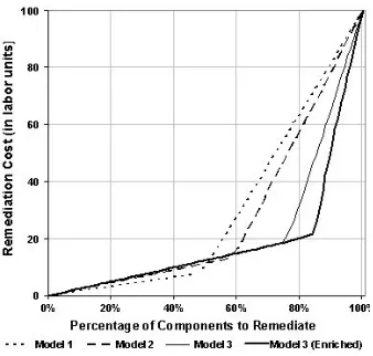
We show the resulting cost curves, using the sequential approach described above, for Models 1, 2, 3, and Model 3-Enriched in Figure 4. The y-axis represents the total (cumulative) cost in terms of labor units to fortify a given percentage of attack-prone components. (The y axis values are normalized to a maximum of 100 to protect the confidentiality of the underlying system data.) The cost curve for Model 1 shows that engineers would incur a lower cost to find 49% of the attack-prone components than by using any of the other models, but Model 1 becomes more expensive than Model 3 as the percentage exceeds 49%. Further work is needed to determine if our initial cost model performs as well as other similar cost models (e.g., [17]).

Figure 4. Cost curves for four CART models.

Table 8 shows the number of labor units needed to remediate a given percentage of attack-prone components, in a system of 100 components. For example, using Model 3-Enriched to repair 80% of the attack-prone components would require 20.3 resource units. If a remediation budget can accommodate 52.0 resource units for this purpose, one can use the same model, Model 3-Enriched, to identify which components to remediate in order to ensure repairing 90% of the attack-prone components in the system.

Table 8. Remediation levels for four CART models.

Remediation level

Model 20% 40% 60% 80% 90% 100%

1 3.2 6.5 28.1 64.0 81.6 100.0 2 4.5 9.1 16.3 58.2 78.6 100.0 3 5.0 9.9 14.9 32.3 65.8 100.0 3-Enriched 5.0 9.9 14.9 20.3 52.0 100.0

8. Summary

We created and evaluated three predictive models based on data from a Cisco software system. One model identifies 75.6% of the attack-prone components

in 18.6% percent of the system’s components. The models substantially reduce the search space for security efforts, which enables security engineers to prioritize their efforts on the small subset of attack-prone components. We have applied cost models and sequential CART analyses to further reduce the costs of remediating components.

9. Acknowledgment

This work is supported by the National Science Foundation under CAREER Grant No. 0346903. Any opinions, findings and conclusions or recommendations expressed in this material are those of the authors and do not necessarily reflect the views of the National Science Foundation.

10. References

[1]O. H. Alhazmi, Y. K. Malaiya, and I. Ray, "Measuring, analyzing and predicting vulnerabilities in software systems,"

Computers & Security, vol. 26, no. 3, pp. 219-228, May

2006.

[2]B. Boehm, Software Engineering Economics, New Jersey, Prentice-Hall, 1981.

[3]B. Boehm and V. Basili, "Software Defect Reduction Top 10 List," IEEE Computer, vol. 34, no. 1, pp. 135-137, January, 2001.

[4]P. Chandra, B. Chess, and J. Steven, "Putting the Tools to Work: How to Succeed with Source Code Analysis," IEEE Security & Privacy, vol. 4, no. 3, pp. 80-83, May/June, 2006. [5]B. Chess and J. West, Secure Programming with Static

Analysis, Boston, MA, Addison Wesley, 2007.

[6]J. L. Devore, Probability and Statistics for Engineering

and the Sciences, Belmont, CA, Thomson, 2008.

[7]E. Dijkstra, Structured Programming, Brussels, Belgium, 1970.

[8]R. Freund, R. Littell, and L. Creighton, Regression Using JMP, Cary, NC, SAS Institute, Inc., 2003.

[9]M. Gegick, "Failure-prone Components are also Attack-prone Components," OOPSLA - ACM student research

competition, Nashville, Tennessee, pp. 917-918, October

2008.

[10]M. Gegick and L. Williams, "STUDENT PAPER: Ranking Attack-prone Components with a Predictive Model," ISSRE, Redmond, WA, pp. 315-316, November 2008.

[11]M. Gegick, L. Williams, J. Osborne, and M. Vouk, "Prioritizing Software Security Fortification through Code-Level Security Metrics," Workshop on Quality of Protection, Alexandria, VA, pp. 31-37, October 2008.

[12]M. Gegick, L. Williams, and M. Vouk, "Predictive Models for Identifying Software Components Prone to Failure During Security Attacks," Build Security In (https://buildsecurityin.us-cert.gov/daisy/bsi/home.html) 2008.

[14]T. Hastie, R. Tibshirani, and J. H. Friedman, The

Elements of Statistical Learning, New York, Springer, 2001.

[15]ISO, "ISO/IEC DIS 14598-1 Information Technology - Software Product Evaluation - Part 1: General Overview," October 28 1996.

[16]ISO/IEC 24765, "Software and Systems Engineering Vocabulary," 2006.

[17]Y. Jiang, B. Cukic, and T. Menzies, "Cost Curve Evaluation of Fault Prediction Models," ISSRE, Redmond, WA, 11-14 November 2008.

[18]T. M. Khoshgoftaar, E. B. Allen, and J. Deng, "Using Regression Trees to Classify Fault-Prone Software Modules,"

IEEE Transactions on Reliability, vol. 51, no. 4, pp. 455-562,

December 2002.

[19]R. Littell, W. Stroup, and R. Freund, SAS for Linear

Models, Fourth Edition, Cary, NC., SAS Institute, Inc., 2002.

[20]G. McGraw, Software Security: Building Security In, Boston, Addison-Wesley, 2006.

[21]MITRE, "Common Weakness Enumeration," http://cwe.mitre.org/, 2006.

[22]H. Motulsky, Intuitive Biostatistics, New York, Oxford University Press, 1995.

[23]N. Nagappan and T. Ball, "Static Analysis Tools as Early Indicators of Pre-release Defect Density," ICSE, St. Louis, MO, pp. 580-586, 2005.

[24]N. Nagappan and T. Ball, "Use of Relative Code Churn Measures to Predict Defect Density," ICSE, St. Louis, MO, pp. 284-292, 15-21 May 2005.

[25]S. Neuhaus, T. Zimmermann, C. Holler, and A. Zeller, "Predicting Vulnerable Software Components," CCS, Alexandria, VA, pp. 529-540, 29 October-2 November 2007. [26]T. J. Ostrand, E. J. Weyuker, and R. M. Bell, "Where the bugs are," ISSTA, Boston, Massachusetts, pp. 86-96, 2004. [27]A. Ozment and S. Schechter, "Milk or wine: does software security improve with age?," 15th Conference on

USENIX Security Symposium, pp. 93-104, July 2006.

[28]SAS Institute Inc., "The Partition Platform," SAS Institute, Inc., Cary, NC, 2003.

[29]M. Vouk and K. C. Tai, "Some Issues in Multi-Phase Software Reliability Modeling," CASCON, Toronto, pp. 512-523, October 1993.

[30]I. Witten and E. Frank, Data Mining, Second ed. San Francisco, Elsevier, 2005.

[31]M. Young and R. N. Taylor, "Rethinking the Taxonomy of Fault Detection Techniques," ICSE, pp. 53-62, 1989. [32]J. Zheng, L. Williams, W. Snipes, N. Nagappan, J. Hudepohl, and M. Vouk, "On the Value of Static Analysis Tools for Fault Detection," IEEE Transactions on Software