A General Statistical Framework for Mapping Quantitative Trait Loci in Nonmodel Systems: Issue for Characterizing Linkage Phases

(1)



A General Statistical Framework for Mapping Quantitative Trait Loci in

Nonmodel Systems: Issue for Characterizing Linkage Phases

Min Lin,* Xiang-Yang Lou,*

,†

**_{Myron Chang* and Rongling Wu*}**

,‡,1

*Department of Statistics, University of Florida, Gainesville, Florida 32611,†_{Department of Agronomy, Zhejiang University,} Hangzhou, Zhejiang 310029, People’s Republic of China and‡_{Laboratory of Statistical Genetics,}

Zhejiang Forestry College, Lin’An, Zhejiang 311300, People’s Republic of China Manuscript received July 13, 2002

Accepted for publication June 17, 2003

ABSTRACT

Because of uncertainty about linkage phases of founders, linkage mapping in nonmodel, outcrossing systems using molecular markers presents one of the major statistical challenges in genetic research. In this article, we devise a statistical method for mapping QTL affecting a complex trait by incorporating all possible QTL-marker linkage phases within a mapping framework. The advantage of this model is the simultaneous estimation of linkage phases and QTL location and effect parameters. These estimates are obtained through maximum-likelihood methods implemented with the EM algorithm. Extensive simulation studies are performed to investigate the statistical properties of our model. In a case study from a forest tree, this model has successfully identified a significant QTL affecting wood density. Also, the probability of the linkage phase between this QTL and its flanking markers is estimated. The implications of our model and its extension to more general circumstances are discussed.

R

ECENT developments of modern molecular marker The theory behind this interval-mapping method was subsequently extended to create a so-called composite-technologies and statistical and computational

tools have led to a great resurgence of interest in study- interval mapping by combining multiple marker re-gression analysis techniques, which can overcome the ing the inheritance and genetic architecture of a

com-influences of QTL in other different marker intervals plex trait at the individual quantitative trait locus (QTL)

(reviewed inJansen2000). Although these two statisti-level (Landerand Schork 1994; Lander and

Wein-cal developments of QTL mapping have brought about berg2000;Mackay2001). A number of analytical

meth-numerous publications on QTL identification, they are odologies that suit different situations of QTL mapping

not designed to make a simultaneous search for all have been framed (Lynch and Walsh 1998; Jansen

possible QTL affecting a quantitative trait throughout 2000;Weller2001) and the results of genetic analysis

the entire genome.KaoandZeng(1997) have derived for a variety of organisms using these methodologies

general formulas for obtaining maximum-likelihood es-have been reported (reviewed inWuet al.2000;Mackay

timates for QTL positions and effects. In their article, the 2001). According to the biological properties of study

authors developed a multiple-interval-mapping method to objects, all these theoretical or empirical studies can be

search and map all possible QTL by analyzing multiple classified into two categories, one for model systems and

marker intervals simultaneously and, therefore, to esti-the oesti-ther for nonmodel systems.

mate the genetic architecture of a quantitative trait in QTL mapping for model systems, in which

homozy-a comprehensive frhomozy-amework. gous inbred lines can be developed, is performed with

Unlike the model systems, it is difficult or impossible well-designed experiments. One popular experimental

to generate inbred lines in nonmodel systems and, thus, design is to create a segregating progeny population,

QTL mapping for these species should be based on such as F2 or backcross, by using two complementary

existing nondomesticated populations, such as a full-sib inbred lines. Statistical technologies for identifying QTL

family derived from heterozygous parents (Grattapag-in these standard designs are relatively simple because

liaandSederoff 1994). In the mapping populations there are only two segregating alleles for each genetic locus

of nonmodel systems the number of segregating alleles and because the allelic frequencies and linkage phases for

per marker locus or QTL and linkage phases between both the markers and QTL are known. Lander and

different loci are usually unknown. These two uncertain-Botstein (1989) for the first time proposed a

maxi-ties make linkage analysis and QTL mapping using mo-mum-likelihood-based method to map a QTL in a

chro-lecular markers much more challenging for a full-sib mosomal interval bracketed by two flanking markers.

family of outbred lines than for a progeny of a cross derived from inbred lines. Several studies have been conducted for linkage analyses of molecular markers

1_{Corresponding author:}_{Department of Statistics, 533 McCarty Hall C,}

University of Florida, Gainesville, FL 32611. E-mail: [email protected] of a different amount of segregation informativeness

(2)

(Ritteret al.1990;Aruset al.1994;RitterandSala- the cross, a total of 18 possible cross types exist for a segregating marker locus (Table 1). On the basis of both mini1996;Maliepaardet al.1997;Ridoutet al.1998)

or QTL identification using these different markers in parental and offspring marker band patterns, these cross types can be classified into seven groups:

a full-sib family (Scha¨fer-Pregl et al. 1996; Johnson et al. 1999; Song et al. 1999). In some studies, more

A. Loci that are heterozygous in both parents and segre-sophisticated statistical algorithms, such as Bayesian

ap-gate in a 1:1:1:1 ratio, including four alleles,ab ⫻ proaches relying on a Markov chain Monte Carlo, have

cd; three nonnull alleles, ab ⫻ ac; three nonnull been proposed to take the complexity of full-sib family

alleles and a null allele,ab⫻co; and two null alleles mapping into account (Hoescheleet al.1997;Sillanpaa

and two nonnull alleles,ao⫻ bo. and Arjas 1999; Xu and Yi 2000). However, all these

B. Loci that are heterozygous in both parents and segre-studies are still simplified in practice because they do not

gate in a 1:2:1 ratio, which include three groups: provide a robust approach for characterizing linkage

B1. Three alleles form a nonsymmetrical cross type phases between markers and QTL. Because different

between the two parents. Of the three alleles, segregation patterns are expected under different

link-one is a null allele in link-one parent, e.g.,ab⫻ao. age phases (Wuet al. 2002), the failure to characterize

B2. The reciprocal of B1. a correct linkage phase may lead to serious biases for

B3. Two alleles form a symmetrical type between the the estimation of QTL positions and effect sizes in a

two parents,i.e.,ab⫻ab. full-sib family.

C. Loci that are heterozygous in both parents and segre-In this article, we extendWuet al.’s (2002) multilocus

gate in a 3:1 ratio,i.e.,ao⫻ao. analysis procedure to simultaneously estimate linkage

D. Loci that are in the testcross configuration between and linkage phases between markers and QTL

segregat-the parents and segregate in a 1:1 ratio, which in-ing in outcrossin-ing populations. Our idea here is to

inte-clude two groups: grate all possible linkage phases between a putative QTL

D1. Heterozygous in one parent and homozygous in and two flanking markers in two parents, each specified

the other, including three alleles, ab ⫻ cc; two by a phase probability, within the framework of a

mix-alleles,ab⫻ aa,ab⫻oo, andbo⫻ aa; and one ture statistical model. In characterizing a most likely

alleleao⫻oo. linkage phase on the basis of the phase probabilities, the

D2. The reciprocals of D1. QTL position, QTL effects, and other model parameters

A general statistical framework has been proposed are also estimated using a likelihood approach. We

per-for linkage analysis of different types of markers in non-form numerous simulation studies to investigate the

model systems (Wuet al. 2002). A multilocus linkage robustness, power, and precision of our statistical

map-phase inference model is derived on the basis of a hid-ping method, incorporating linkage phases. An

exam-den Markov chain process to simultaneously estimate ple from an outcrossing forest tree is used to validate

linkage and linkage phases for the markers on a same the application of our method to QTL mapping for

linkage group. The genetic mapping of QTL is con-nonmodel systems.

ducted using such a well-constructed linkage map.

A general framework:Consider two outbred parental

STATISTICAL MODEL _{lines denoted as}_P_and_Q_{, each containing two}

homolo-Marker segregation types:A commonly used mapping _{gous chromosomes}₁₂_{in a set. The cross between these}

population for outcrossing species is one derived from _{two lines,}₁₂_⫻₁₂_{, results in four possible parental} chro-a full-sib fchro-amily generchro-ated by two heterozygous outbred _{mosome pairings,}₁₁_,₁₂_,₂₁_{, and}₂₂_{. In this article, we} parental lines. In such a full-sib family, many different _{used italic numbers to denote parental chromosomes.} marker segregation types can be expected given the As explained above and seen in Table 1, there may heterozygosity of the two parents. Grattapagliaand be many different marker types in a full-sib family de-Sederoff(1994) proposed a well-accepted pseudo-test rived from the two outbred parental lines. However, all backcross design for mapping in an outcrossing popula- observed markers, no matter which type they come tion, but this design can use only a portion of the ge- from, can be described by two alleles, Mk

1 and Mk2, at nome markers segregating in one parent but null in marker ᏹk _{and two alleles,} _Mk⫹1

1 and Mk2⫹1, at marker the other. For a full-sib family derived from two outbred ᏹk⫹1 _{for parent} _P_{. Similarly, the corresponding alleles} parents, up to four marker alleles, besides a null allele, for parentQ are described asNk

1 andNk2at markerᏹk at a single locus, can occur. Also, the number of alleles andNk⫹1

(3)

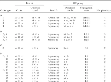
TABLE 1

Possible marker genotype cross combinations and observed marker band patterns for parents and their offspring

Parent Offspring

Observed Observed Segregation

Cross type Cross band Remark bands ratio No. phenotypes

A

1 ab⫻cd ab⫻cd Asymmetry ac,ad,bc,bd 1:1:1:1 4

2 ab⫻ac ab⫻ac Asymmetry a,ac,ba,bc 1:1:1:1 4

3 ab⫻co ab⫻c Asymmetry ac,a,bc,b 1:1:1:1 4

4 ao⫻bo a⫻b Asymmetry ab,a,b,o 1:1:1:1 4

B

B15 ab⫻ao ab⫻a Asymmetry ab, 2a,b 1:2:1 3

B26 ao⫻ab a⫻ab Asymmetry ab, 2a,b 1:2:1 3

B37 ab⫻ab ab⫻ab Symmetry a, 2ab,b 1:2:1 3

C

8 ao⫻ao a⫻a Symmetry 3a,b 3:1 2

D

D1 9 ab⫻cc ab⫻c Asymmetry ac,bc 1:1 2

10 ab⫻aa ab⫻a Asymmetry a,ab 1:1 2

11 ab⫻oo ab⫻o Asymmetry a,b 1:1 2

12 bo⫻aa b⫻a Asymmetry ab,a 1:1 2

13 ao⫻oo a⫻o Asymmetry a,o 1:1 2

D214 cc⫻ab c⫻ab Asymmetry ac,bc 1:1 2

15 aa⫻aa a⫻ab Asymmetry a,ab 1:1 2

16 oo⫻ab o⫻ab Asymmetry a,b 1:1 2

17 aa⫻bo a⫻b Asymmetry ab,a 1:1 2

18 oo⫻ao o⫻a Asymmetry a,o 1:1 2

Marker types B3and C each have the same genotypes in both parents and, therefore, are called symmetrical

marker cross types. The other marker types have parent-specific marker genotypes and are called asymmetrical marker cross types. Marker cross types D1and D2are called two-way pseudo-test backcrosses (Grattapaglia

andSederoff1994).

ing a 1:1:1:1 ratio in the family. The recombination fractions between the two markers, between marker

⌽12⫽ Mk

1

P1 Mk⫹1

1

冨

Mk

2

P2 Mk⫹1

2

冨

⫻

Nk

1

Q2 Nk⫹1

1

冨

Nk

2

Q1 Nk⫹1

2

冨

→ (P1Q2,P1Q1,P2Q2,P2Q1),

ᏹk _{and the QTL and between the QTL and marker}

ᏹk⫹1_{, are denoted by}_r_,_r_{1, and}_r_{2, respectively, with}_r⫽ r1 ⫹ r2 ⫺ 2r1r2. Parent-specific difference of linkage is ignored. The alleles of these two markers and the QTL are arranged between the two homologous

chromo-⌽21⫽ Mk

1

P2 Mk⫹1

1

冨

Mk

2 P1 Mk⫹1

2

冨

⫻

Nk

1 Q1 Nk⫹1

1

冨

Nk

2 Q2 Nk⫹1

2

冨

→ (P2Q1,P2Q2,P1Q1,P1Q2), somes in each of a total of four possible linkage phases

for each parent. But the allelic linkage phases of the two markers can be known for both parents through linkage analyses of markers using a strategy proposed inWuet al.(2002). Thus, under a fixed-marker linkage

⌽22⫽ Mk

1

P2 Mk⫹1

1

冨

Mk

2

P1 Mk⫹1

2

冨

⫻

Nk

1

Q2 Nk⫹1

1

冨

Nk

2

Q1 Nk⫹1

2

冨

→ (P2Q2,P2Q1,P1Q2,P1Q2), phase, we will have 2⫻ 2 ⫽ 4 parental combinations

(⌽’s) of linkage phase of the QTL relative to the two markers, schematically expressed, along with the order

where the first and second subscripts of⌽denote two of the four QTL genotypes in the progeny, as

possible phases of parents P and Q, respectively, and the vertical lines for each phase combination denote two parental chromosomes 12 for each parent. Each ⌽11⫽

Mk

1

P1 Mk⫹1

1

冨

Mk

2

P2 Mk⫹1

2

冨

⫻

Nk

1

Q1 Nk⫹1

1

冨

Nk

2

Q2 Nk⫹1

2

冨

(4)

with the gamete probabilities depending on the phase. the joint probabilities of the 64 zygotic genotypes (and therefore the conditional probabilities of the QTL geno-Under phase combination⌽11, the eight gamete

proba-bilities are calculated as types given marker genotypes) will be different among the four phase combinations. However, regardless of the

g111⫽Prob(M1kP1Mk1⫹1)⫽Prob(Nk1Q1Nk1⫹1)⫽ 1

2(1⫺r1)(1⫺r2), difference among these four phase combinations, these conditional probabilities under different phase

combi-g112⫽Prob(M1kP1Mk2⫹1)⫽Prob(Nk1Q1Nk2⫹1)⫽ 1

2(1⫺r1)r2, nations can be obtained just by changing the order of the QTL genotypes corresponding to a particular phase

2r1r2, combination (Table 2).

Letuandvdenote the QTL alleles that an offspring

2r1(1⫺r2), i has received from parentP andQ, respectively. The conditional probability of the QTL genotype for this

2r1(1⫺r2), individual under parental-phase combination⌽11is de-noted by huvi expressed in one of the four vectors,

2r1r2, h

k(k⫹1)

11 , hk12(k⫹1), h21k(k⫹1), and hk22(k⫹1). The probability with which a particular phase occurs is denoted as p for

2(1⫺r1)r2, parentPandqfor parentQ. Without loss of generality, let φ11⫽ pq,φ12⫽p(1⫺ q), φ21⫽ (1⫺ p)q, andφ22⫽

2(1⫺r1)(1⫺r2), (1⫺ p)(1⫺ q). Thus, the conditional probability of a QTL genotype PuQv in the full-sib family should be a

where we use the subscripts to denote the marker and mixture of the corresponding conditional probabilities QTL alleles. The eight gametes from parent P unite under these four phase combinations, weighted byφ11, randomly with the eight gametes from parentQ, which _φ12,φ21, andφ22.

will generate a total of 64 zygotic genotypes. The proba- Assume that the phenotypic valuesyof a QTL geno-bilities of the joint genotypes for the two markers and type PuQv are normally distributed with mean ␮uv and

the QTL are calculated on the basis of theg’s, which are _variance _␴2_{, expressed as} _f

uv(yi)⫽ 1/

√

2␲␴exp[⫺(yi⫺

expressed in matrixGk(k⫹1)_{(Table 2). This joint probability} _␮

uv)2/2␴2]. The likelihood function of the phenotypic

matrix is composed of four vectors,gk(k⫹1)

11 ,gk12(k⫹1),g21k(k⫹1), values (y) for all N offspring in the full-sib family is and gk(k⫹1)

22 , each corresponding to a different parental expressed in terms of a normal mixture model: chromosomal pairing. The probabilities of the 2-marker

L(⍀|y)⫽

兿

N i⫽1

[(h11iφ11⫹h12iφ12⫹h21iφ21⫹h22iφ22)f11(yi),

gametic genotypes are expressed as

⫹(h12iφ11⫹h11iφ12⫹h22iφ21⫹h21iφ22)f12(yi)

g1·1⫽Prob(Mk1Mk1⫹1)⫽Prob(Nk1Nk1⫹1)⫽ 1 2(1⫺r)

⫹(h21iφ11⫹h22iφ12⫹h11iφ21⫹h12iφ22)f21(yi)

g1·2⫽Prob(Mk1Mk2⫹1)⫽Prob(Nk1Nk2⫹1)⫽ 1

2r ⫹(h22iφ11⫹h21iφ12⫹h12iφ21⫹h11iφ22)f22(yi)]

2r ⫽

兿

N i⫽1

兺

2

u⫽1

兺

2

v⫽1

␲uvifuv(yi),

(1)

2(1⫺r). where⍀⫽(␮uv,␴

2_,_p_,_q₎T_{is the vector for unknown} parame-ters contained within the mixture model, and ␲11i ⫽

h11iφ11⫹h12iφ12⫹h21iφ21⫹h22iφ22,␲12i⫽h12iφ11⫹h11iφ12⫹ These 4 marker gametic probabilities are used to calculate

h22iφ21⫹h21iφ22,␲21i⫽ h21iφ11⫹h22iφ12⫹h11iφ21⫹h12iφ22,

16 marker zygotic probabilities denoted by vectorMk(k⫹1)_.

and␲22i⫽h22iφ11⫹h21iφ12⫹h12iφ21⫹h11iφ22are the mix-Thus, according to Bayes theorem, the matrix (Hk(k⫹1)_{) for}

ture of the conditional probabilities of different QTL the conditional probabilities of different QTL genotypes,

genotypes over different phase combinations. The pa-conditional upon the marker interval genotypes, can be

rameters contained in ⍀ can be estimated by imple-derived as

menting the expectation-maximization (EM) algorithm

Hk(k⫹1)⫽_Gk(k⫹1)⭋_Mk(k⫹1)_,

(Dempsteret al.1977). The log-likelihood of Equation 1 is given by

where ⭋ stands for the division of the corresponding

elements of each column in a matrix by a column vector. _log _L₍_⍀_|_y₎_⫽

_兺

N

i⫽1 log

冤

兺

2

u⫽1

兺

2

v⫽1

␲uvifuv(yi)

冥

(2)

Correspondingly, the conditional probability matrixHk(k⫹1) is composed of four vectors, hk(k⫹1)

11 , hk12(k⫹1), hk21(k⫹1), and _{with a derivative for any unknown}_⍀

␭

hk(k⫹1)

22 , each represented by a different parental

chromo-somal pairing. ⳵

⳵⍀␭logL(⍀|y)⫽

兺

N

i⫽1

兺

2

u⫽1

兺

2

v⫽1

␲uvi(⳵/⳵⍀␭)fuv(yi)

兺

2

u⫽1

兺

2

v⫽1␲uvifuv(yi)

(5)

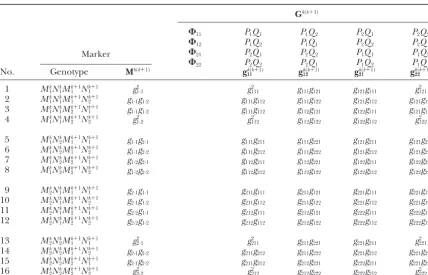
TABLE 2

A 16-dimensional vector (Mk(kⴙ1)_{) for the probabilities of the marker genotypes for}ᏹk_andᏹkⴙ1_{and a}

(16⫻4)-matrix (Gk(kⴙ1)_{) for the probabilities of the joint genotypes for the two markers} and the QTL bracketed by the markers in a full-sib family

Gk(k⫹1)

⌽11 P1Q1 P1Q2 P2Q1 P2Q2

⌽12 P1Q2 P1Q1 P2Q2 P2Q1

⌽21 P2Q1 P2Q2 P1Q1 P1Q2

⌽22 P2Q2 P2Q1 P1Q2 P1Q1

Marker

No. Genotype Mk(k⫹1) _gk(k⫹1)

11 gk12(k⫹1) g21k(k⫹1) gk22(k⫹1)

1 Mk

1Nk1Mk1⫹1Nk1⫹1 g21·1 g2111 g111g121 g121g111 g2121

2 Mk

1Nk1M1k⫹1Nk2⫹1 g1·1g1·2 g111g112 g111g122 g121g112 g121g122

3 Mk

4 Mk

1Nk1Mk2⫹1Nk2⫹1 g21·2 g2112 g112g122 g122g112 g2122

5 Mk

6 Mk

7 Mk

8 Mk

9 Mk

10 Mk

11 Mk

12 Mk

13 Mk

2Nk2Mk1⫹1Nk1⫹1 g22·1 g2211 g211g221 g221g211 g2221

14 Mk

15 Mk

16 Mk

2Nk2Mk2⫹1Nk2⫹1 g22·2 g2212 g212g222 g222g212 g2222

The order of zygotic genotypes in the full-sib family under different phase combinations⌽11–⌽22is given,

and the conditional probabilities matrix (Hk(k⫹1)_{) of the QTL genotypes upon the marker genotypes can be}

calculated according to Bayes theorem.

is estimated by treatingr1 (and therefore r2) as fixed. ⫽

_兺

N

i⫽1

兺

2

u⫽1

兺

2

v⫽1

␲uvifuv(yi)

兺

2

u⫽1

兺

2

v⫽1␲uvifuv(yi)

⳵

⳵⍀␭log

fuv(yi) Using a grid approach, we can obtain the MLE of the

QTL location from the peak of the profile of the log-likelihood ratio test statistics across a chromosome. ⫽

_兺

N

i⫽1

兺

2

u⫽1

兺

2

v⫽1

兿

uvi

⳵

⳵⍀␭log

fuv(yi) ,

On the basis of quantitative genetic theory, the geno-typic value of a QTL can be partitioned into the additive where we define _{and dominant effects as}

兿

uvi⫽

␲uvifuv(yi)

兺

2

u⫽1

兺

2v⫽1␲uvifuv(yi)

, (3) _␮uv⫽ ␮ ⫹ ␣u⫹ ␤v⫹ ␦uv,u,v⫽1, 2,

where ␮is the overall mean, ␣uand ␤vare the allelic

which could be thought of as a posterior probability that

(additive) effects of alleles u and v, respectively, and theith offspring has a QTL genotypePuQv. We then

imple-␦uv is the interaction (dominant) effect at the QTL.

ment the EM algorithm with the expanded parameter set

Considering all possible alleles and allele combinations {⍀,⌸}, where⌸⫽{⌸uvi}. Conditional on⌸, we solve for

between the two parents, there are a total of four addi-the zeros of (⳵/⳵⍀φ) logL(⍀|y) (appendix a) to get our

tive effects (␣1and␣2from parentPand␤1and␤2from estimates of ⍀ (the M step). The estimates are then

parentQ) and four dominant effects (␦11,␦12, ␦21, and used to update⌸ (the E step), and the process is

re-␦22). But these additive and dominant effects are not peated until convergence. The values at convergence

independent and, therefore, are not estimable. After pa-are the maximum-likelihood estimates (MLEs).

rameterization, there are two independent additive effects, Because marker information for each offspring has

␣ ⫽ ␣1 ⫽ ⫺␣2 and␤ ⫽ ␤1 ⫽ ⫺␤2, and one dominant been incorporated into the mixture model of Equation

effect,␦ ⫽ ␦11⫽ ⫺␦12⫽ ⫺␦21⫽ ␦22, to be estimated. 1, one unknown parameterr1orr2(that determines the

Letm⫽(␮uv)4⫻1anda⫽(␮,␣,␤,␦)T, which can be location of the QTL on the interval) should be estimated

(6)

m⫽ Da, can be formulated for testing for the significance of any kind of gene effects of the QTL detected.

where _{In a full-sib family derived from two outbred parents,}

it is possible that a putative QTL does not segregate in a 1:1:1:1 ratio. The genetic model (1) proposed in this

D⫽

冤

1 1 1 1

1 1 ⫺1 ⫺1 1 ⫺1 1 ⫺1 1 ⫺1 ⫺1 1

冥

. article has power to test if the QTL detected is diallelic segregating 1:2:1 (like marker type B) or 1:1 (like marker type D1or D2; see Table 1). The hypothesis that a signifi-The MLE ofacan be obtained from the MLE ofmby cant QTL conforms to segregation type B can be tested

by formulating

aˆ ⫽D⫺1_m_ˆ_.

H0:␣ ⫽ ␤

Fitting marker phenotypes:We have built a general

H1:␣⬆␤. framework for QTL mapping based on the two-marker

zygote genotypes. But in practice only the phenotypes _{Similarly, the hypothesis for testing for the} consis-of the marker zygotes can be observed. The numbers _{tency of the QTL segregation to type D can be} formu-of the zygote phenotypes formu-of a marker are 4, 3, 3, 3, 2, _{lated as}

2, and 2 for marker types A, B1, B2, C, D1, and D2,

H0:␣ ⫽0 or␤ ⫽0 respectively (Table 1). We have designed different

inci-dence matricesI(Wuet al.2002;appendix b) to connect _{H1: Neither of them equals zero.} the zygotic genotypes to the zygotic phenotypes for all

In each of the two hypotheses above, the LR is calcu-different marker types listed in Table 1. Thus, general

lated similarly to Equation 4. In practice, the segregation expressions for the probability vector of two-marker

ge-pattern of a significant QTL should be tested because notypes or the joint probability matrix of two markers

this is important for designing an efficient breeding and QTL for particular marker types can be derived by

strategy. using the corresponding incidence matrices (appendix

b), which are expressed as

MONTE CARLO SIMULATION

M·k(k⫹1)⫽ ₍_Ik 丢

Ik⫹1₎_Mk(k⫹1)_,

Extensive simulation studies are performed to test the

G·k(k⫹1)⫽ ₍_Ik丢_Ik⫹1₎_Gk(k⫹1)_,

statistical properties of our method for simultaneously where丢 is the Kronecker product, andIk_and_Ik⫹1 _are _{estimating QTL position and effects and linkage phase} the incidence matrices for markers ᏹk _and ᏹk⫹1_{. For} _{between the QTL and markers in an outcrossed} popula-some marker types, the pattern and structure of the tion. Suppose a full-sib family is derived from two out-incidence matrices are dependent on the linkage phases crossed parents. This full-sib family is genotyped at six of the two flanking markers. Hence, the conditional equally spaced (20-cM) fully informative markers (type probability matrix for an observed marker type is calcu- A), forming five intervals. A QTL is hypothesized at 26 lated as cM from the first marker (located within the second

interval).

H·k(k⫹1)⫽_G·k(k⫹1)⭋_M·k(k⫹1)_,

The phenotypic values for this full-sib family are simu-lated by giving a particular set of unknown QTL effect which is used as a basis for QTL mapping in outcrossing

parameters under the linkage phase combination ⌽11 species.

for the two parents. These simulated data are subject

Hypothesis tests: The existence of a QTL of

signifi-to mapping analysis using our model that considers a cant effect within a marker interval can be tested by

mixture of all possible linkage phases. Thus, if the MLEs calculating a log-likelihood ratio (LR) test statistic under

of the phase probabilities p and q are near one, this the null (H0, there is no QTL) and alternative

hypothe-indicates that our model can precisely characterize the ses (H1, there is a QTL), expressed as

linkage phase for a practical phase-unknown data set. LR⫽ ⫺2[logL0(␮11⫽ ␮12⫽ ␮21⫽ ␮22⫽ ␮˜ ,␴˜2,φ˜j) Of course, if the data are simulated under the other

linkage phase combination, the values of p and q

re-⫺logL1(⍀ˆ)]. (4)

flecting this correct linkage phase should be changed The LR under the null hypothesis is asymptotically correspondingly.

(7)

cates can be approximated by a ␹2 _{distribution. The} _{somal pairings, the maximums of the LR values from} the correct linkage phase⌽11and the three incorrect 99th percentile of the distribution of the maximum is

used as empirical critical values to declare chromosome- linkage phases ⌽12, ⌽21, and ⌽22 will be identical (see Figure 2), suggesting that phase-separate analyses have wide existence of a significant QTL at the significance

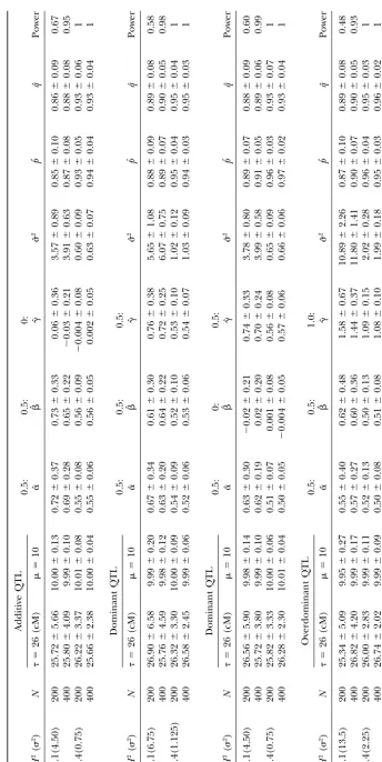
level␣ ⫽0.01. no power to select a most likely linkage phase. Also as shown by flat, crooked curves, the maximum LR value Our simulation schemes include different gene action

modes (additive, dominant, or overdominant), differ- from a single linkage phase model cannot be used to precisely determine the QTL position. Figure 2 also ent heritabilities (H2⫽_{0.1 or 0.4), and different sample}

sizes (N ⫽ 200 or 400; Table 3). Given a heritability illustrates the LR values across the linkage group calcu-lated when all linkage phase combinations are consid-and the genetic variance calculated from hypothesized

genetic effect values, we estimate the residual variance ered simultaneously on the basis of the same simulated data set. A higher peak of the curve for a mixed-phase (␴2_{). The accuracy and precision of parameter estimates}

are affected by gene action modes in three ways (Table analysis (see also Figure 1B) indicates that our model has a greater advantage in detecting a significant QTL 3). First, an overdominant QTL tends to have a more

precise estimate of location than does a dominant or than usual phase-separate analyses do. When an incor-rect linkage phase is used, the signs of the MLEs of the additive QTL. For example, the standard error (SE) of

the location MLE for an overdominant QTL is 14–20% additive and dominant effects of a QTL will be reversed (results not shown).

smaller than those for other QTL when the heritability is 0.4 and sample size is 400. Second, for a small heritability trait, the MLEs of additive effects for an overdominant

A CASE STUDY

QTL are less biased than those for additive or dominant

QTL. Third, the dominant effect is overestimated to a We use an example of an outcrossed forest tree to demonstrate the power of our statistical model for map-larger extent than the additive effect, especially for an

overdominant QTL. ping QTL affecting a quantitative trait. The study mate-rial used was derived from the hybridization between The estimation accuracy and precision of all

parame-ters can be improved when heritabilities and sample two poplar species,Populus deltoidesandP.euramericana. A genetic linkage map was constructed using a so-called sizes are increased (Table 3). For example, it is difficult

to estimate the position of QTL for a low heritability pseudo-testcross strategy (GrattapagliaandSederoff 1994) based on 90 genotypes selected randomly from (H2⫽_{0.1) trait when}_N⫽_{200 (Figure 1A). An increased}

sample size (N⫽400) can lead to more precise estima- the F1interspecifc hybrid family with random amplified polymorphic DNAs (RAPDs), amplified fraction length tion of the QTL location. For a high heritability (H2⫽

0.4) trait, the QTL can be precisely localized, especially polymorphisms (AFLPs), and intersimple sequence re-peats (ISSRs;Yinet al.2002). This map is composed of when a larger sample size is used (Figure 1B). Similar

trends also hold for the estimates of other QTL parame- the 19 largest linkage groups for each parental map, which roughly represent 19 pairs of chromosomes. The ters, such as additive and dominant effects, and model

parameters (overall means and residual variance; Table 90 hybrid genotypes used for map construction were measured for wood density with wood samples collected 3). It appears that there are more substantial

improve-ments in the accuracy and precision of parameter esti- from 11-year-old stems in a field trial. The measurement for each genotype was repeated four to six times to mates due to an increased heritability level from 0.1 to

0.4 than to an increased sample size from 200 to 400. reduce measurement errors. The means of these geno-types were calculated and used for QTL mapping here. It is interesting to note that our model can well

esti-mate the linkage phase between the QTL and the mark- Our model can successfully identify a significant QTL for wood density on linkage group D17 as reported in ers. The MLEs of phase probabilities are close to 0.90

for a small heritability trait andⱖ0.95 for a high herita- Yinet al.(2002). In this example, the empirical estimate of the critical value is obtained from 1000 permutation bility trait (Table 3). Unlike the estimation of other

param-eters, the power of detecting a significant QTL seems tests. It is found that the critical value for declaring the existence of a QTL on the whole linkage group under to be more sensitive to sample sizes than to heritabilities

(Table 3). For a small mapping population, the power consideration is 6.9 at the significance level P ⫽ 0.05. The profile of the LRs of the full vs. reduced model of detecting a significant QTL is considerably reduced.

We also performed an additional simulation experi- across the length of linkage group D17 has a steep peak between a narrow marker interval AG/CGA-480–AG/ ment to test the influence of incorrectly characterizing

a linkage phase on QTL detection and parameter esti- CGA-330 (Figure 3). The LR value at this peak is 11.7, well beyond the empirical critical threshold at the sig-mation. The simulated data, givenH2 ⫽ _{0.4 and}_N ⫽

400, under linkage phase combination⌽11are analyzed nificance levelP ⫽0.05.

The additive effect of this significant QTL detected using models based on this phase and three other

(8)

(9)

Figure 1.—The profiles of the log-likelihood ratio (LR) test statistic from one random simulation repli-cate for QTL detection across a linkage group for a quantitative trait with differ-ent heritabilities (A) H2_⫽

0.1 and (B)H2_⫽_{0.4. The}

statistical model used con-siders all possible linkage phases between the QTL and its flanking markers (second and third marker). Results from different sam-ple sizes (N⫽200, broken curves;N⫽400, solid curves) are compared. The empirical thresholds for declaring the existence of a QTL at the significant level 0.05 are indicated by two horizonal lines (N⫽200, broken lines;N⫽ 400, solid lines). The vertical lines with an arrow indicate the position of the hypothesized QTL. The additive and dominant effects of a QTL hypothesized in the model are␣ ⫽ 0.5,␤ ⫽0.5, and␦ ⫽0.5.

variance for wood density in hybrid poplars. The MLE of publications reporting on the detection of QTL in of phase probabilitypis 0.82, thus suggesting that there different species (Wu et al.2000; Mackay2001). Yet, is quite a high probability to have a linkage phase⌽11. despite significant importance, QTL mapping in out-This indicates that the positive allele of this QTL that crossing species is often frustrated due to lack of an increases wood density is, at a probability of 0.82, in appropriate statistical method to consider high hetero-coupling phase with dominant alleles of the two markers zygosity of this group of species. In this article, we pres-AG/CGA-480 and AG/CGA-330 flanking the QTL. ent a statistical model for mapping QTL in these out-The same material was analyzed using a traditional inter- crossing, nonmodel systems by incorporating their val-mapping approach that assumes a possible QTL- heterozygous nature into a mapping framework. marker linkage phase at one time. This phase-separate Our model is advantageous over current QTL map-approach can also identify a significant QTL for wood ping methods in a full-sib family derived from outcross-density (data not shown), but cannot determine a cor- ing species in three aspects (Andersson et al. 1994; rect linkage phase because the maximums of the LR Haleyet al. 1994;Xu 1996; Knottet al. 1997). First, values are identical between two possible linkage phases. our model can characterize a correct linkage phase be-Our method provides important information about nonal- tween a putative QTL and markers. For heterozygous lelic arrangements on the homologous chromosomes. populations, allelic arrangements of different markers and QTL on a single chromosome,i.e., linkage phase, generally cannot be knowna priori. The current

statisti-DISCUSSION

cal methods for full-sib analysis either were based on a simplified assumption that markers are segregating but Statistical strategies for mapping QTL segregating in

QTL fixed in a full-sib family (Haley et al. 1994) or an inbred population have been well established

(re-viewed in Jansen 2000), which has led to a number failed to consider the influence of incorrectly

character-Figure2.—The profiles of the log-likelihood ratio (LR) test sta-tistic from one random simulation replicate for QTL detection across a linkage group under one mixed-(solid curve) and four separate-phase analyses (dotted curves). The heritability for the trait hy-pothesized isH2_⫽_{0.4 with a}

(10)

Figure3.—The profile of the log-likelihood ratio (LR) test statistic for QTL detection across linkage group D17 in Yin et al. (2002), using the mixed-phase analysis. The empiri-cal threshold based on per-mutation tests (Churchill and Doerge 1994) is indi-cated at the horizonal line. The marker names across the linkage group are given at the bottom.

izing a marker-QTL linkage phase on parameter estima- not only important for parameter estimation and model selection, but also essential for the application of molec-tion when both markers and QTL are assumed to be

segregating (Knottet al.1997). Linkage phase affects ular results to genetic improvement programs. For a genetic breeding program, we need to know the direc-statistical inference about QTL effect size and direction

for a fixed-model approach, although this problem does tion of genetic effects to make an efficient marker-assisted selection. Suppose a dominant marker allele is not occur for a random model-based mapping approach

(XuandAtchley1995). in a coupling phase with the positive allele of a QTL. Thus, the selection for dominant marker alleles can Second, our model can analyze all possible different

types of markers and can test how a QTL is segregating lead to improved phenotypes due to favorable QTL alleles. Without this knowledge, however, it is possible in a family. Most of the current studies consider only

fully informative markers. For example,Xu(1996) pro- to select the negative allele of this QTL by using the marker allele if it is based only on the significant rela-posed a full-sib family-mapping approach by assuming

four different alleles at each marker and QTL. This tionship between the marker and QTL.

The robustness and performance of our statistical approach is likely limited because the genome of an

outcrossing species is often covered by different types method has been examined through extensive simula-tions. One of the most important findings is that im-of polymorphism markers, forming many different cross

types when two parents are crossed (Table 1). Third, provements in the accuracy and precision of QTL pa-rameters can be more substantial with increased our model provides a way of simultaneously estimating

linkage phases and QTL parameters within a unified heritabilities than with increased sample sizes (Table 2). In practice, this conclusion will have important impli-framework. Simulation studies suggest that this unified

framework has power to characterize a most likely link- cations for framing an optimal experiment design for precise estimation of QTL parameters. To increase pa-age phase and also displays increased power to detect

a significant QTL (Figure 2). For two heterozygous par- rameter precision, for example, special care should be paid to the use of silvicultural measurements to increase ents used to generate a full-sib family, there are multiple

linkage phases, but only one is correct. For pure marker site homogeneity, rather than planting a huge sample size on large-scale, nonuniform sites.

analysis, maximum-likelihood approaches can be used

to select a most likely linkage phase because different The model proposed is based on simple interval map-ping for a single QTL affecting a quantitative trait using phases correspond to different LR values (Wu et al.

2002). But, using two markers to infer a QTL, all differ- a mixed set of marker types. The theory extended to capture information provided by other markers outside ent linkage phases theoretically give the identical LR

(Figure 2), which indicates that it is not possible to interval markers considered is straightforward (seeZeng 1994) and simulations can be similarly conducted to test correctly detect a linkage phase on the basis of

likeli-hood analysis. If QTL identification is based on a wrong the analytical advantages and disadvantages of including more markers in our analysis model. Also, a more impor-linkage phase, the estimation of QTL additive and

domi-nant effects will have an inverse sign. tant statistical aspect of QTL-mapping models is to si-multaneously map multiple linked QTL for a trait. Mul-The correct characterization of a linkage phase

(11)

MLEs and the asymptotic variance-covariance matrix in mapping reality because many traits are actually polygenic (Lynch

quantitative trait loci when using the EM algorithm. Biometrics andWalsh1998) and can also increase the power to _53:_653–665.

Knott, S. A., D. B. Neale, M. M. SewellandC. S. Haley, 1997 detect QTL of smaller effects from an analytical

perspec-Multiple marker mapping of quantitative trait loci in an outbred tive. Several QTL may be located on the same linkage

pedigree of loblolly pine. Theor. Appl. Genet.94:810–820. group or different groups. In addition to the modeling _{Lander, E. S}_{., and}_{D. Botstein}_{, 1989} _{Mapping Mendelian factors}

underlying quantitative trait using RFLP linkage maps. Genetics of more gene actions and interactions between different

121:185–199. QTL, multiple-QTL analyses include increased linkage

Lander, E. S., andN. J. Schork, 1994 Genetic dissection of complex phase combinations relative to the marker intervals on _{traits. Science}_265:_2037–2048.

Lander, E. S., andR. A. Weinberg, 2000 Genomics: journey to the which different QTL are located. It is possible that these

center of biology. Science287:1777–1782. more complex models can be solved using Markov chain

Lynch, M., andB. Walsh, 1998 Genetics and Analysis of Quantitative Monte Carlo algorithms (Robert and Casella 1999; _Traits_{. Sinauer, Sunderland, MA.}

Mackay, T. F. C., 2001 The genetic architecture of quantitative Sillanpaa and Arjas 1999; Xu and Yi 2000). For a

traits. Annu. Rev. Genet.35:303–339. broader application, we have proposed a unified

frame-Maliepaard, C., J. JansenandJ. W. van Ooijen, 1997 Linkage work for simultaneous maximum-likelihood estimation _{analysis in a full-sib family of an outbreeding plant species:} over-view and consequences for applications. Genet. Res.70:237–250. of linkage phases and QTL actions and interactions in

Ritter, E., andF. Salamini, 1996 The calculation of recombination our computer program.

frequencies in crosses of allogamous plant species with applica-tions to linkage mapping. Genet. Res.67:55–65.

This work is partially supported by an Outstanding Young

Investiga-Ritter, E., C. GebhardtandF. Salamini, 1990 Estimation of re-tors Award of the National Science Foundation of China (30128017),

combination frequencies and construction of RFLP linkage maps a University of Florida Research Opportunity Fund (02050259), and

in plants from crosses between heterozygous parents. Genetics a University of South Florida Biodefense grant (7222061-12) to R.W.,

125:645–654. and National Science Foundation of China grant (30000097) to

Ridout, M. S., S. Tong, C. J. VowdenandK. R. Tobutt, 1998 Three-X.-Y.L. The publication of this manuscript is approved as journal _{point linkage analysis in crosses of allogamous plant species.} series no. R-09202 by the Florida Agricultural Experiment Station. _{Genet. Res.}_72:_111–121.

Robert, C. P., andG. Casella, 1999 Monte Carlo Statistical Methods. Springer, New York.

Scha¨fer-Pregl, R., F. SalaminiandC. Gebhardt, 1996 Models

LITERATURE CITED _{for mapping quantitative trait loci (QTL) in progeny of}

non-inbred parents and their behaviour in presence of distorted

segre-Andersson, L., C. S.Haley, H.Ellegren, S. A.Knott, M.Johansson

gation ratios. Genet. Res.67:43–54.

et al., 1994 Genetic mapping of quantitative trait loci for growth

Sillanpaa, M. J., andE. Arjas, 1999 Bayesian mapping of multiple and fatness in pigs. Science263:1771–1774.

quantitative trait loci from incomplete outbred offspring data.

Arus, P., C. Olarte, M. RomeroandF. Vargas, 1994 Linkage

Genetics151:1605–1619. analysis of 10 isozyme genes in F1segregating almond progenies.

Song, J. Z., M. SollerandA. Genizi, 1999 The full-sib intercross J. Am. Soc. Hort. Sci.119:339–344.

line (FSIL): a QTL mapping design for outcrossing species.

Churchill, G. A., and R. W. Doerge, 1994 Empirical threshold

Genet. Res.73:61–73. values for quantitative trait mapping. Genetics138:963–971.

Weller, J. I., 2001 Quantitative Trait Loci Analysis in Animals. CABI

Dempster, A. P., N. M. LairdandD. B. Rubin, 1977 Maximum

Publishing, New York. likelihood from incomplete data via EM algorithm. J. R. Stat.

Wu, R., C.-X. Ma, I. PainterandZ-B. Zeng, 2002 Simultaneous Soc. Ser. B39:1–38.

maximum likelihood estimation of linkage and linkage phases

Grattapaglia, D., andR. Sederoff, 1994 Genetic linkage maps of

in outcrossing species. Theor. Popul. Biol.61:349–363.

Eucalyptus grandis andEucalyptus urophyllausing a

pseudo-test-Wu, R. L., Z-B. Zeng, S. M. McKeandandD. M. O’Malley, 2000 The cross: mapping strategy and RAPD markers. Genetics137:1121–

case for molecular mapping in forest tree breeding. Plant Breed.

1137. _Rev._19:_41–68.

Haley, C. S., S. A.Knottand J. M.Elsen, 1994 Mapping

quantita-Xu, S. Z., 1996 Mapping quantitative trait loci using four-way crosses. tive trait loci in crosses between outbred lines using least squares. _{Genet. Res.}_68:_175–181.

Genetics136:1195–1207. _{Xu, S. Z}_{., and}_{W. R. Atchley}_{, 1995} _{A random model approach to}

Hoeschele, I., P. Uimari, F. E. Grignola, Q. ZhangandK. M. Gage, _{interval mapping of quantitative trait loci. Genetics}_141:_1189– 1997 Advances in statistical methods to map quantitative trait _1197.

loci in outbred populations. Genetics147:1445–1457. _{Xu, S}_{., and}_{N. Yi}_{, 2000} _{Mixed model analysis of quantitative trait}

Jansen, R. C., 2000 Quantitative trait loci in inbred lines, pp. 567– _{loci. Proc. Natl. Acad. Sci. USA}_97:_{14542–14547.}

597 inHandbook of Statistical Genetics, edited by D. J.Balding, M. _{Yin, T. M., X. Y. Zhang, M. R. Huang, M. X. Wang, Q. Zhuge}

Bishopand C.Cannings. John Wiley & Sons, New York. _{et al.}_{, 2002} _{The molecular linkage maps of the}_Populus_genome.

Johnson, D. L., R. C. JansenandJ. A. M. Van Arendonk, 1999 Map- _Genome_45:_541–555.

ping quantitative trait loci in a selectively genotyped outbred _{Zeng, Z}_-_B_{., 1994} _{Precision mapping of quantitative trait loci.} Genet-population using a mixture model approach. Genet. Res. 73: _ics_136:_1457–1468.

75–83.

Kao, C.-H., andZ-B. Zeng, 1997 General formulas for obtaining the Communicating editor: S.Tavare´

APPENDIX A

We present the formulas for obtaining the MLEs of the unknown parameters⍀⫽(␮uv,␴2,φj)Tin the M step. For

the distribution parameters within the mixture model, we have

␮ˆuv⫽

兺

N i⫽1

兿

uviyi

兺

N i⫽1

兿

uvi

,

␴ˆ2⫽ 1 N

兺

N

i⫽1

兺

2

u⫽1

兺

2

v⫽1

兿

(12)

For the phase probabilities, we have

p⫽

兺

N

i⫽1(␲12␲22⌬1Ki2⫹ ␲11␲21⌬2Ji2)

兺

N

i⫽1[␲12␲22⌬1(Ki2⫺Ki1)⫺ ␲11␲21⌬2(Ji2⫺Ji1)] ,

q⫽

兺

N

i⫽1(␲12␲22⌬⬘1Ki⬘2⫹ ␲11␲21⌬⬘2J⬘i2)

兺

N

i⫽1[␲12␲22⌬⬘1(K⬘i2⫺Ki⬘1)⫺ ␲11␲21⌬⬘2(J⬘i2⫺J⬘i1)]

,

where

⌬1⫽q(h11⫺ h21)⫹(1 ⫺q)(h12⫺h22), ⌬2⫽q(h12⫺ h22)⫹(1 ⫺q)(h11⫺h21),

Ki1⫽q(h21⌸i11⫺h11⌸i21)⫹ (1⫺q)(h22⌸i11⫺ h12⌸i21), Ki2⫽q(h11⌸i11⫺ h21⌸i21)⫹(1 ⫺q)(h12⌸i11⫺h22⌸i21),

Ji1⫽q(h22⌸i12⫺ h12⌸i22)⫹(1 ⫺q)(h21⌸i12⫺h11⌸i22),

Ji2⫽q(h12⌸i12⫺h22⌸i22)⫹ (1⫺q)(h11⌸i12⫺h21⌸i22),

⌬⬘1 ⫽p(h11⫺h12)⫹(1⫺p)(h21⫺h22), ⌬⬘2 ⫽p(h21⫺ h22)⫹ (1⫺p)(h11⫺ h22),

K⬘i1⫽p(h12⌸i11⫺ h11⌸i12)⫹(1 ⫺p)(h22⌸i11⫺h21⌸i12),

K⬘i2⫽p(h11⌸i11⫺ h21⌸i12)⫹(1 ⫺p)(h21⌸i11⫺h22⌸i12),

J⬘i1⫽p(h22⌸i21⫺h21⌸i22)⫹ (1⫺p)(h12⌸i21⫺h11⌸i22),

J⬘i2⫽p(h21⌸i21⫺h22⌸i22)⫹(1 ⫺p)(h11⌸i21⫺h12⌸i22).

APPENDIX B

The pattern and structure of an incidence matrix (Ik_{) relating the zygotic genotypes to phenotypes for marker}

Mk_{depend on the type of this marker (Table 1). When marker}_Mk_{is from marker types A, B1, B2, B3, C, D1, and}

D2, we have

Ik

A⫽

冤

1 0 0 0 0 1 0 0 0 0 1 0 0 0 0 1

冥

,

Ik

B1⫽

       

冤

1 1 0 0 0 0 1 0 0 0 0 1

冥

ifMk

1⫽ Nk1andNk2⫽oor Mk1⫽ Nk2andNk1⫽o

冤

1 0 0 0 0 1 0 0 0 0 1 1

冥

ifMk

2⫽Nk1 andNk2⫽ oorMk2⫽Nk2 andNk1⫽ o,

Ik

B2⫽

       

冤

1 0 1 0 0 1 0 0 0 0 0 1

冥

ifMk

1⫽ Nk1andMk2⫽ oorMk2⫽Nk1 andMk1⫽ o

冤

1 0 0 0 0 1 0 1 0 0 0 1

冥

ifMk

(13)

Ik

B3⫽

       

冤

1 0 0 0 0 1 1 0 0 0 0 1

冥

ifMk

1 ⫽Nk1andMk2 ⫽Nk2

冤

1 0 0 1 0 1 0 0 0 0 0 1

冥

ifMk

1⫽ Nk2andMk2⫽ Nk1,

Ik

C⫽

         

冤

1 1 1 0

0 0 0 1

冥

ifMk1⫽Nk1

冤

1 1 0 1

0 0 1 0

冥

ifM

k

1⫽Nk2

冤

1 0 1 1

0 1 0 0

冥

ifM

k

2⫽Nk1

冤

1 0 0 0

0 1 1 1

冥

ifM

k

2⫽Nk2,

Ik

D1 ⫽

冤

1 1 0 0 0 0 1 1

冥

,

Ik

D2 ⫽

冤

(14)