ABSTRACT
LIU, SHU. On Convergence of the Hardy Cross Method of Moment Distribution. (Under the direction of John Baugh.)
The Hardy Cross method of moment distribution is an iterative method that calculates the moments at member ends of statically indeterminate beams and frames. It was published by
Professor Hard Cross in the early 1930s and soon became widely adopted by engineers around
the world since then. The calculations of the method can be easily performed by hand. The rapid convergence of the method in practice made it possible for engineers to estimate end moments
in just a couple of iterations. Interestingly, while engineers have relied on the correctness and
convergence of the method, formal proofs were not published until recent years.
Although the method has largely been superseded by the convenience and availability of
more general computational approaches, like the direct stiffness method, for decades it was the
primary tool to efficiently and safely design many reinforced concrete buildings.
There are several features of the method that make it interesting from a computational point
of view. These features include but are not limited to multiprocess oriented domain decomposition,
natural parallelism, and scheduling. These features are shared with more challenging problem domains, so the otherwise simplicity of the Hardy Cross method makes it a useful vehicle for
studies of those features. Looking at the family of potential distribution sequences—that is, the
order in which the calculations are performed—convergence issues arise. For instance, what are the most relaxed conditions on distribution sequences necessary for convergence? From the
literature, it appears this question remains unanswered.
Two common types of distribution sequences are used interchangeably by engineers when applying the Hardy Cross method. One is a simultaneous joint balancing distribution sequence,
a Jacobi-like iteration in which calculations in the current iteration are based on results from
the prior iteration. The other is a consecutive joint balancing distribution sequence, a Gauss-Seidel-like iteration in which calculations use the most recently updated values in the current
iteration. While the convergence properties of these two types of distribution sequences have
been characterized, individually, a mathematical treatment of their relationship to each other and to other distribution sequences has not been undertaken.
From physical intuition, a valid distribution sequence for the Hardy Cross method is arbitrary as long as every joint gets updated infinitely often. From a computational point of view, the
Hardy Cross method can be relaxed even further. There are benefits if these arbitrary sequences
and more relaxed forms of the method always converge to the same result for any problem statement. First, the nature of the Hardy Cross method can be more broadly understood as a
method in its more relaxed form can be established.
This thesis proves the equivalence of arbitrary distribution sequences as long as moments at each joint are balanced infinitely often. A more relaxed version of the Hardy Cross method is
also introduced. Similarly, this thesis proves that this more relaxed form always converges to
the same result for any particular problem statement. The proofs are performed by focusing on the mathematical properties of the corresponding iterate matrices without resorting to physical
analogies. In addition, several possible computational implementations of the method, as well
as their relationships to matrix forms, are provided. These include traditional ones based on Jacobi-like and Gauss-Seidel-like iterations, as well as a more relaxed form implemented as a
©Copyright 2015 by Shu Liu
On Convergence of the Hardy Cross Method of Moment Distribution
by Shu Liu
A thesis submitted to the Graduate Faculty of North Carolina State University
in partial fulfillment of the requirements for the Degree of
Master of Science
Civil Engineering
Raleigh, North Carolina
2015
APPROVED BY:
DEDICATION
BIOGRAPHY
Shu Liu was born in 1990 in Fujian, China. He graduated from University of Sydney in Australia in 2012 with a bachelor degree in civil engineering before beginning the Master of Science
ACKNOWLEDGEMENTS
I would like to thank Dr. John Baugh for his generous support and patient guidance throughout my study at NC State. I would also like to thank Dr. Murthy Guddati and Dr. Pierre Gremaud
TABLE OF CONTENTS
LIST OF TABLES . . . vii
LIST OF FIGURES . . . .viii
Chapter 1 Introduction . . . 1
Chapter 2 Background. . . 4
2.1 Hardy Cross Method of Moment Distribution . . . 4
2.2 Jacobi Iteration . . . 6
2.3 Gauss-Seidel Iteration . . . 6
2.4 Convergence of Hardy Cross Method with Simultaneous Joint Balancing . . . 7
Chapter 3 Distribution Sequence and Iteration . . . 10
3.1 Simultaneous Joint Balancing Distribution Sequence and Jacobi Iteration . . . . 11
3.2 Consecutive Joint Balancing Distribution Sequence and Gauss-Seidel Iteration . . . 12
3.3 Arbitrary Distribution Sequence and Arbitrary Sequence Iteration . . . 13
Chapter 4 Iterate Matrix Representation. . . 14
4.1 Jacobi Iterate Matrix Representation . . . 14
4.1.1 General Parameters and Notations . . . 14
4.1.2 Distribution Matrix . . . 15
4.1.3 Carryover Matrix . . . 16
4.1.4 E Matrix . . . 16
4.1.5 Iterate Matrix . . . 17
4.2 Gauss-Seidel Iterate Matrix Representation . . . 18
4.2.1 Iterate Matrix . . . 18
4.2.2 Properties of the Iterate Matrix . . . 18
Chapter 5 Relaxed Hardy Cross Method Convergence Conditions . . . 20
5.1 Relaxed Sufficient Condition . . . 21
5.1.1 Arbitrary Sequence Iteration Matrix Representation . . . 21
5.1.2 Relaxed Sufficient Condition . . . 22
5.2 More Relaxed Sufficient Condition . . . 24
5.2.1 Further Decomposition of E Matrix . . . 25
6.3 Asynchronous Shared Memory Parallel Implementation with Simple Termination 39
6.3.1 Flow Chart . . . 39
6.3.2 Python Code Snippets . . . 40
6.3.3 Example . . . 42
Chapter 7 Termination Detection. . . 46
7.1 Process Priorities . . . 46
7.2 Quiescence Detection . . . 47
7.3 Snapshot of Global State . . . 47
7.4 Generic Techniques for Distributed Computation . . . 48
7.4.1 Dijkstra’s Ring-Based Termination Detection Algorithm . . . 48
7.4.2 Asynchronous Shared Memory Parallel Implementation with Dijkstra’s Termination Detection Algorithm . . . 50
Chapter 8 Conclusions. . . 53
REFERENCES . . . 55
APPENDICES . . . 57
Appendix A Equivalence of Jacobi and Gauss-Seidel Iterations Example . . . 58
Appendix B Python Implementation Source Code . . . 61
B.1 Sequential Implementation File . . . 61
B.2 Asynchronous Shared Memory Parallel Implementation with Simple Termi-nation File . . . 64
LIST OF TABLES
LIST OF FIGURES
Figure 3.1 Two Members and Three Joints Structure with Initial Fixed-End Moments . 10
Figure 6.1 Two Members and Three Joints Structure with Initial Fixed-End Moments . 32 Figure 6.2 Graph Representation of Two Members and Three Joints Structure . . . 32
Chapter 1
Introduction
The Hardy Cross method of moment distribution [Cross, 1930, Cross and Morgan, 1932] is an iterative method that calculates the moments at member ends of statically indeterminate beams
and frames. It is based on a principle that the sum of all the moments at member ends at a
non-fixed joint is zero when a structure is in static equilibrium. Professor Hardy Cross published the method in the early 1930s, several years after he began teaching it to his students at the
University of Illinois [McCormac, 1975]. Afterward, the method was widely adopted by engineers
around the world. It is still being taught in many undergraduate structural analysis courses. Even today, while computers and structural engineering software can efficiently solve many
thousands of simultaneous equations, practicing engineers sometimes still use the Hardy Cross
method to check those results by hand.
There are several reasons why the method became so popular and pervasive in such a
short amount of time. Before the invention of the method, engineers usually needed to set up
and solve equations based on physical principles, which involve equilibrium, compatibility, and force-displacement relations. For structures of realistic size, such computations were burdensome
since, at that time, they had to be performed by hand. In contrast, the steps of the moment
distribution method are easy to remember and to carry out with pencil and paper. The rapid convergence of the method in practice made it possible for engineers to estimate the member
end moments in just a few iterations.
studies of those features. Looking at the family of potential distribution sequences—that is, the
order in which the calculations are performed—convergence issues arise. For instance, what are the most relaxed conditions on distribution sequences necessary for convergence? From the
literature, it appears this question remains unanswered.
Two common types of distribution sequences are used interchangeably by engineers when applying the Hardy Cross method. One is a simultaneous joint balancing distribution sequence,
a Jacobi-like iteration in which calculations in the current iteration are based on results from
the prior iteration. The other is a consecutive joint balancing distribution sequence, a Gauss-Seidel-like iteration in which calculations use the most recently updated values in the current
iteration. While the convergence properties of these two types of distribution sequences have
been characterized, individually, a mathematical treatment of their relationship to each other and to other distribution sequences has not been undertaken.
From physical intuition, a valid distribution sequence for the Hardy Cross method is arbitrary
as long as every joint gets updated infinitely often. From a computational point of view, the Hardy Cross method can be relaxed even further. There are benefits if these arbitrary sequences
and more relaxed forms of the method always converge to the same result for any problem
statement. First, the nature of the Hardy Cross method can be more broadly understood as a family of algorithms. Second, the sufficient conditions needed to guarantee convergence of the
method in its more relaxed form can be established.
This thesis proves the equivalence of arbitrary distribution sequences as long as moments at
each joint are balanced infinitely often. A more relaxed version of the Hardy Cross method is
also introduced. Similarly, this thesis proves that this more relaxed form always converges to the same result for any particular problem statement. The proofs are performed by focusing on
the mathematical properties of the corresponding iterate matrices without resorting to physical
analogies. In addition, several possible computational implementations of the method, as well as their relationships to matrix forms, are provided. These include traditional ones based on
Jacobi-like and Gauss-Seidel-like iterations, as well as a more relaxed form implemented as a
multiprocess algorithm.
The organization of this thesis is as follows. After this introductory chapter, the second
includes background on the Hardy Cross method. The third chapter defines and includes
examples of (1) the simultaneous joint balancing distribution sequence and Jacobi iteration, (2) the consecutive joint balancing distribution sequence and Gauss-Seidel iteration, as well as (3) a
more general case, namely arbitrary distribution sequence and arbitrary sequence iteration. The
forth chapter describes matrix representations of different types of distribution sequences and iteration in detail. Afterward, it lists several important properties of these matrices, some of
which will be used for subsequent proofs. The fifth chapter introduces and proves two relaxed
can be more broadly understood. The sixth chapter provides several possible computational
implementations of the method in the Python programming language, as well as their relationship to the matrix form. While the asynchronous parallel implementation in the sixth chapter uses
simple termination criteria, the seventh chapter lists various more sophisticated termination
Chapter 2
Background
2.1
Hardy Cross Method of Moment Distribution
The moment distribution method published by Professor Hardy Cross in the early 1930s is useful for finding end moments in a structure, usually statically indeterminate beams and frames, in an
iterative way [Cross, 1930]. In his 1930 paper, Professor Hardy Cross described the distribution
sequence of this joint-by-joint method, referred to here as the simultaneous joint balancing distribution sequence, as follows:
1. Imagine all joints in the structure are clamped so that they cannot rotate. Under this
condition, compute the moments, which are called the initial fixed-end moments, at the
ends of each member based on loads on members.
2. Release each non-fixed joint simultaneously by calculating its unbalanced moments, and then redistribute these unbalanced moments among the connecting members in proportion
to their stiffness. The unbalanced moment is the algebraic sum of the fixed-end moments
at each joint. The relative stiffness of connecting members are called distribution factors.
3. Calculate the carryover moments by multiplying the redistributed moments by the carryover factors, then add this carryover moment to the far end of each member.
4. Repeat step 2 and 3 until the changes in moments are small enough to be neglected, and the results are the true moments at the ends.
The method with the simultaneous joint balancing distribution sequence can be written in a
form of an infinite series of matrix productions. More than three decades later, based on the
rediscovered by a group of researchers [Lopes et al., 2005] apparently unaware of Mozingo’s
publication.
However, while the Hardy Cross method with the simultaneous joint balancing distribution
sequence provides remarkable convergence in practice, a proof of its convergence was not published
until much more recently [Volokh, 2002]. Volokh characterizes the method with the simultaneous joint balancing distribution sequence as a Jacobi iterative scheme. He starts with the classical
displacement method of a structure and then shows an incremental form of the Jacobi iterative
scheme that can be used to solve these simultaneous equations. By using a specific starting point, the incremental form of Jacobi iterative scheme can represent the process of applying the
Hardy Cross method with the simultaneous joint balancing distribution sequence. Because of
the diagonal dominance of the stiffness matrix from the displacement method’s simultaneous equations, the Jacobi iteration—and equivalently the Hardy Cross method—converges for any
loading condition. Section 2.4 illustrates these mathematical transformations in detail.
Professor Hardy Cross introduced another type of distribution sequence in a subsequent pub-lication [Cross and Morgan, 1932], referred to here as theconsecutive joint balancing distribution
sequence. While the simultaneous joint balancing distribution sequence does not have a direct
physical interpretation, the consecutive one does and can be used in the Hardy Cross method to better visualize the nature of the operations being performed [West, 1989]. Instead of calculating
and adding the carryover moments after releasing all joints simultaneously, these steps are performed incrementally, one joint at a time. Thus every step in this consecutive joint balancing
distribution sequence represents a real physical operation of releasing and clamping of a joint.
Based on this type of distribution sequence, the method can be characterized as a Gauss-Seidel iteration [Guo, 1987]. Like Volokh after him, Guo starts with the classical displacement method
of a structure and then presents an incremental form of the Gauss-Seidel iterative scheme that
can be used to solve its simultaneous equations. Similarly, the Hardy Cross method with the consecutive joint balancing distribution sequence matches this incremental form of Gauss-Seidel
iteration with a specific starting point. Due to the fact that the stiffness matrix from the
simultaneous equations is positive definite, the Gauss-Seidel iteration—and equivalently the Hardy Cross method—converges for any loading conditions. While Volokh’s overall approach is
similar, he was apparently unaware of Guo’s work.
Unlike the approach taken by Volokh and Guo, this thesis begins with the Hardy Cross method
itself, and then constructs corresponding iterate matrices. It also addresses the equivalence between any arbitrary distribution sequences and iterations, rather than the convergence of
a particular case. Technically speaking, the form of the iterations introduced in this thesis
include standard Jacobi-like and Gauss-Seidel-like iterations, which directly calculate member end moments instead of their increments, a less direct form that requires further analysis.
2.2
Jacobi Iteration
The Jacobi method [Bronshtein et al., 2007] is an iterative technique for solving simultaneous
equations in the formAx=b, where matrixAhas non-zero elements on its main diagonal. In each iteration, each equation—say the ith equation—is solved independently as
n X
j=1
aijxj =bi , (2.1)
which updates the value of xi while leaving the other entries of x unchanged [Black et al., b]. As a result, the value ofxi at the kth iteration can be derived as
x(ik)=
bi−P j6=i
aijx(jk−1) aii
. (2.2)
In each iteration the updates are independent, so the order in which they are performed is irrelevant. Hence, in terms of matrices, the definition of the Jacobi method can be expressed as
x(k)=D−1(L+U)x(k−1)+D−1b , (2.3)
where the matricesD,−L, and−U are the diagonal, strictly lower triangular, and strictly upper triangular parts of A, respectively.
As an alternative approach, the Jacobi iteration can be translated into an incremental form.
The incremental Jacobi iteration deals with the residual, r(k) =b−Ax(k), instead of x itself. When the iteration converges,r tends to be 0, which is actually the solution ofAr= 0.
2.3
Gauss-Seidel Iteration
The Gauss-Seidel method is also an iterative technique for solving simultaneous equations.
as they are available, so the value ofxi at thekth iteration can be derived as
x(ik)=
bi−P j<i
aijx(jk)− P j>i
aijx(k
−1)
j
aii . (2.4)
Consequently, multiple updates cannot be performed simultaneously as in the Jacobi method. Moreover, the order in which they are performed affects the intermediate results. Thus, the
definition of the Gauss-Seidel method can be expressed with matrices as
x(k)= (D−L)−1(U x(k−1)+b) , (2.5)
where the matrices D,−L, and −U again are the diagonal, strictly lower triangular, and strictly upper triangular parts of A, respectively. An incremental form of Gauss-Seidel iteration also exists, which minimizes the norm of the residual as well.
2.4
Convergence of Hardy Cross Method with Simultaneous
Joint Balancing
This section gives a more detailed review of the approach taken by Volokh, which begins with
the displacement method for solving the following canonical system of equilibrium equations
Ku+p= 0, (2.6)
whereK is a stiffness matrix, uis a nodal displacement vector, and pis a nodal loads vector. From physical principles, the matrix K is symmetric and diagonally dominant, and can be written as
Kii= m X
j=1,i6=j
Mij (2.7)
and
Kij = 1 2Mij =
1
2Mji, (2.8)
Further, Eq. 2.9 has a component-wise form of
u(ik+1)=−Kii−1 m X
j=1,i6=j
(Kiju(jk)+pi). (2.10)
The starting point of the iteration, u(0), does not affect the convergence of the Jacobi iteration. Let
u(0)i = 0, (2.11)
then
u(1)i =−Kii−1pi. (2.12)
Define
∆u(ik)=ui(k+1)−u(ik), (2.13) then we have
∆u(0)i =u(1)i −u(0)i =−Kii−1pi (2.14) and
ui =X
k
∆u(ik). (2.15)
Thus we can transform Eq. 2.10 into incremental form as
∆u(ik+1) =−Kii−1 m X
j=1,i6=j
Kij∆u(jk). (2.16)
Pre-multiplying Eq. 2.16 by Mij and rearranging the equation we get
Mij∆u(ik+1) =−K
−1
ii Kij m X
j=1,i6=j
Mij∆u(jk). (2.17)
Substituting Eq. 2.7 and Eq. 2.8 into Eq. 2.17 and letting
∆Mi,j(k) =Mij∆u(jk), (2.18)
then Eq. 2.17 results in the form
∆Mij(k+1)=− mMij
P j=1,i6=j
Mij m X
j=1,i6=j
∆Mij(k)
2 . (2.19)
Chapter 3
Distribution Sequence and Iteration
An entire family of distribution sequences may be used in the Hardy Cross method, though this more general form has not been demonstrated to be correct. A distribution sequence is actually
a sequence of releases or a procedure of cross-carryover. This chapter defines and includes
examples of (1) the simultaneous joint balancing distribution sequence and Jacobi iteration, (2) the consecutive joint balancing distribution sequence and Gauss-Seidel iteration, as well as (3)
a more general case, namely arbitrary distribution sequence and arbitrary sequence iteration.
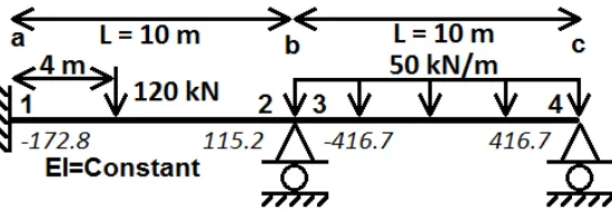
Step-by-step results are demonstrated for these iterations by applying them to the structure shown in Figure 3.1 [West, 1989].
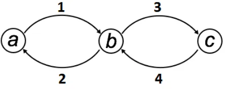
Figure 3.1: Two Members and Three Joints Structure with Initial Fixed-End Moments
It is a simple structure consisting of 3 joints (a, b, and c) and 4 ends (1, 2, 3, and 4). The
initial fixed-end moments are -172.8, 115.2, -416.7, and 416.7 kN/m, the distribution factors are 0, 0.5, 0.5, and 1, and the carryover factors are 0, 0.5, 0.5, and 0.5 for end 1, 2, 3, and 4
respectively. These fixed-end moments, distribution factors, and carryover factors are calculated
3.1
Simultaneous Joint Balancing Distribution Sequence and
Jacobi Iteration
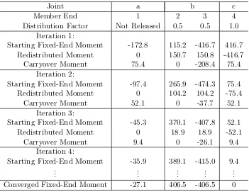
The simultaneous joint balancing distribution sequence is defined such that in one cycle, all non-fixed joints are balanced simultaneously exactly once, then the carryover moments are
recorded simultaneously as well. Its corresponding iteration is essentially a Jacobi iteration. In
each iteration, all calculations are based on results from the prior iteration. In other words, moments calculated for joints in the current iteration will not be used until the next iteration.
Table 3.1 lists the step-by-step results of applying this approach to the structure shown in Figure 3.1.
Table 3.1: Step-by-Step Results of Jacobi Iterations
Joint a b c
Member End 1 2 3 4
Distribution Factor Not Released 0.5 0.5 1.0
Iteration 1:
Starting Fixed-End Moment -172.8 115.2 -416.7 416.7
Redistributed Moment 0 150.7 150.8 -416.7
Carryover Moment 75.4 0 -208.4 75.4
Iteration 2:
Starting Fixed-End Moment -97.4 265.9 -474.3 75.4
Redistributed Moment 0 104.2 104.2 -75.4
Carryover Moment 52.1 0 -37.7 52.1
Iteration 3:
Starting Fixed-End Moment -45.3 370.1 -407.8 52.1
Redistributed Moment 0 18.9 18.9 -52.1
Carryover Moment 9.4 0 -26.1 9.4
Iteration 4:
Starting Fixed-End Moment -35.9 389.1 -415.0 9.4
..
. ... ... ... ...
3.2
Consecutive Joint Balancing Distribution Sequence and
Gauss-Seidel Iteration
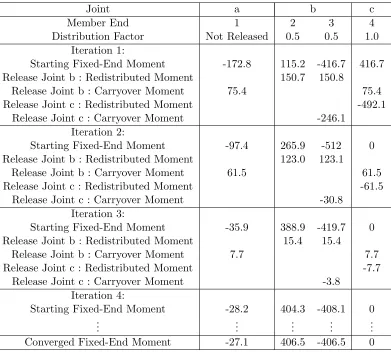
The consecutive joint balancing distribution sequence is defined such that in one cycle, each non-fixed joint is balanced one-by-one exactly once, and the corresponding carryover moments
are recorded immediately after balancing each joint. Its corresponding iteration is essentially a
Gauss-Seidel iteration. In each iteration, all calculations are based on the morst recent available values from either the current or prior iteration. Table 3.2 lists several step-by-step results
of applying Gauss-Seidel iterations on the same structure with a distribution sequence of
joint b→joint cwhile joint ais not released in each iteration.
Table 3.2: Step by Step Results of Gauss-Seidel Iterations
Joint a b c
Member End 1 2 3 4
Distribution Factor Not Released 0.5 0.5 1.0
Iteration 1:
Starting Fixed-End Moment -172.8 115.2 -416.7 416.7
Release Joint b : Redistributed Moment 150.7 150.8
Release Joint b : Carryover Moment 75.4 75.4
Release Joint c : Redistributed Moment -492.1
Release Joint c : Carryover Moment -246.1
Iteration 2:
Starting Fixed-End Moment -97.4 265.9 -512 0
Release Joint b : Redistributed Moment 123.0 123.1
Release Joint b : Carryover Moment 61.5 61.5
Release Joint c : Redistributed Moment -61.5
Release Joint c : Carryover Moment -30.8
Iteration 3:
Starting Fixed-End Moment -35.9 388.9 -419.7 0
Release Joint b : Redistributed Moment 15.4 15.4
Release Joint b : Carryover Moment 7.7 7.7
Release Joint c : Redistributed Moment -7.7
Release Joint c : Carryover Moment -3.8
Iteration 4:
Starting Fixed-End Moment -28.2 404.3 -408.1 0
..
. ... ... ... ...
3.3
Arbitrary Distribution Sequence and Arbitrary Sequence
Iteration
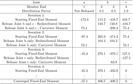
An arbitrary distribution sequence is defined such that in one iteration, some subset of non-fixed joints is balanced simultaneously exactly once, after which the carryover moments are also
recorded simultaneously. Assuming that all joints are be updated infinitely often, no joints are
left unbalanced. Its corresponding iteration is referred to as arbitrary sequence iteration. In each iteration, all calculations are also based on results from the prior iteration. The joints can
be chosen arbitrarily in each iteration, so some may be updated more frequently than others. Actually both Jacobi and Gauss-Seidel methods are special cases of arbitrary sequence iteration.
Table 3.3 again lists a few step-by-step results of applying one possible set of arbitrary sequence
iterations on the same structure.
Table 3.3: Step by Step Results of Arbitrary Sequence Iterations
Joint a b c
Member End 1 2 3 4
Distribution Factor Not Released 0.5 0.5 1.0
Iteration 1:
Starting Fixed-End Moment -172.8 115.2 -416.7 416.7
Release Joint b and c : Redistributed Moment 150.7 150.8 -416.7
Release Joint b and c : Carryover Moment 75.4 -208.4 75.4
Iteration 2:
Starting Fixed-End Moment -97.4 265.9 -474.3 75.4
Release Joint b only: Redistributed Moment 104.2 104.2
Release Joint b only: Carryover Moment 52.1 52.1
Iteration 3:
Starting Fixed-End Moment -45.3 370.1 -370.1 127.5
Release Joint c only: Redistributed Moment -127.5
Release Joint c only: Carryover Moment -63.8
Iteration 4:
Starting Fixed-End Moment -45.3 370.1 -433.9 0
..
. ... ... ... ...
Chapter 4
Iterate Matrix Representation
Jacobi and Gauss-Seidel iterations can be represented in matrix form. This chapter illustrates the constructions of these iterate matrices in detail, then shows several properties of them. Some
of these properties will be used in later chapters to demonstrate convergence conditions.
4.1
Jacobi Iterate Matrix Representation
4.1.1 General Parameters and Notations
This section defines some general parameters and notations that are also used in subsequent
sections. LetN be the number of joints andM the number of member ends. Obviously,M is an even number. Define
p(i) =j
p(j) =i (4.1)
as a mapping between the indexesiand j of the two ends of a member. Eq. 4.1 suggests
i=p(p(i)). (4.2)
LetKi be the stiffness of the member containing endi. Member stiffnesses are not necessarily
symmetric, soKi may not be the same asKp(i). Stiffness is always positive, so
4.1.2 Distribution Matrix
Let matrix D, whose size is M×M, be a distribution matrix of the redistribution process. Let set Si, i= 1,2, . . . , M, be a set containing all ends, includingi itself, that meet at a common joint. For instance, in the prior example ends ab, ba, bc, and cb are numbered 1 through 4, so at joint b we have S2 = {2,3} and S3 = {2,3}. This thesis considers only structures with
N ≥3 and all joints connected together. Hence at least one of the joints has two or more ends connected, e.g.,∃i:size(Si)≥2. Since one end can only be connected to one joint,
Si \
Sj = ∅if and only if end iand end j do not frame into a common joint
Si = Sj if and only if end iand end j frame into a common joint. (4.4)
Let Di be the ith column of D. Letdij be the element atith row and jth column in matrix D.
dij is the ratio between the increment of the moment at end i due to the moment at end j
during the redistribution process. Thus
dij =
0 ifSi6=Sj or endi is connected to a fixed joint − PKi
k∈Si Kk
otherwise (4.5)
that gives Dsome special properties:
1. Dhas multiple identical columns. Particularly, ifSj =Sk, then Dj is identical to Dk,
dij =dik ifSj =Sk . (4.6)
Thus there are at leastsize(Sj) columns identical toDj including itself. Also because of
Eq. 4.4, there is at most one distinct negative value in each row.
2. Dis singular.
3.
0≥dij ≥ −1. (4.7)
4. Column sum ofDi is either 0 if endi is fixed, or -1 otherwise:
M X
j=1
dij = X ∀j:Si=Sj
dij =
(
0 if end iis fixed
−1 otherwise (4.9)
5. Due to Eq. 4.4 and 4.5,
dij <0⇒dp(i),j = 0, (4.10)
which means an end will not be affected by the other end in the same member during the
redistribution process.
4.1.3 Carryover Matrix
Let matrix C be the matrix of carryover factors. Because the carryover moments are only transferred between the two ends of a member,
(
0< cij <1 ifj =p(i)
cij = 0 otherwise
. (4.11)
So matrixCDrepresents the ratio between the carryover moment on one end and the calculated unbalanced moment of the other end in the same member. MatrixCD essentially swaps any two rows inD that correspond to the two ends of a member, and then multiplies each row by the corresponding carryover factor. Also due to Eq. 4.10,D andCD cannot both have negative elements at the same position, e.g.dij×[CD]ij = 0.
4.1.4 E Matrix
Define
E=D+CD (4.12)
and E has some special properties similar to D:
1. E has multiple identical columns. Particularly, ifSj =Sk, then Ej is identical toEk,
eij =eik ifSj =Sk . (4.13)
Thus there are at least size(Sj) columns identical toEj including itself. Also because of
Eq. 4.4, there are at most two distinct negative values in each row.
Moreover, 0> eij ≥ −1 if and only if Si=Sj and the corresponding joint is not fixed, or
endj is connected to the same joint where the other end of the member that has endiis connected to, e.g. j=p(i). This implies
eii=dii (
= 0 if endi is fixed
<0 otherwise (4.15)
and if Si=Sj, then
ep(i),j =cp(i),jeij . (4.16)
4. Column sum ofEi is either 0 if end iis fixed or less than 0 and greater than −2 otherwise.
0≥
M X
j=1
eij = X
∀j:Si=Sj∨j=p(i)
eij >−2 (4.17)
5.
X
∀j:Si=Sj
eij = X ∀j:Si=Sj
dij =
(
0 if end iis fixed
−1 otherwise (4.18)
4.1.5 Iterate Matrix
The Jacobi iterate matrix of the Hardy Cross method, BJ acobi, can be written as
BJ acobi=I+D+CD =I+E (4.19)
and the iteration can be written as
M(k+1) =BJ acobiM(k) (4.20)
where M(k) is a vector representing moments at each member end at step k. The limit of Eq. 4.20 and the Jacobi iteration is1
4.2
Gauss-Seidel Iterate Matrix Representation
4.2.1 Iterate Matrix
For the Gauss-Seidel iteration shown in Section 3.2, the Hardy Cross method can also be
represented as a simple iteration similar to Eq. 4.20 but with a different iterate matrix,BGS. The matrix E can be represented as
E=
N X
l=1
b
El (4.22)
where N is the number of joints, andEbl is a square matrix that contains some columns ofE
that correspond to all ends connected to jointl while the other columns of Ebl are zero.2 The
matrix representing the process of releasing a joint lonce can be written as
b
Bl=I+Ebl . (4.23)
The iterate matrix BGS of Gauss-Seidel iteration can be written as
BGS=
N Y
l=1
b Bl =
N Y
l=1
(I+Ebl) . (4.24)
The iteration can be written as
M(k+1) =BGSM(k) . (4.25)
The limit of Eq. 4.25 and the Gauss-Seidel iteration is
M∗=BGS∞M(0) , (4.26)
where M∗ again is the converged result.
4.2.2 Properties of the Iterate Matrix
Here are some properties of this type of iteration matrix.
Theorem 1. Let Bbl be the matrix representing the process of releasing a joint l once, then Bbl
is idempotent, i.e. Bbl2=Bbl.
Proof. Due to Eq. 4.5, 4.6, 4.16, and 4.18,
(Ebl2)ij = M X
k=1
(Ebl)ik(Ebl)kj = (Ebl)ij M X
k=1
Dkj =−(Ebl)ij , (4.27)
which means 3
b
El2+Ebl= 0 . (4.28)
Then
2Ebl+Ebl2=Ebl
⇒I+ 2Ebl+Ebl2 =I+Ebl
⇒(I+Ebl)2 =I+Ebl
⇒Bbl2=Blb . (4.29)
The physical interpretation of Theorem 1 is that releasing a particular joint consecutively
twice is the same as doing so only once. This make sense because the unbalanced moment will
Chapter 5
Relaxed Hardy Cross Method
Convergence Conditions
This chapter introduces and proves sufficient conditions for the convergence of two more relaxed
forms of the Hardy Cross method. These iterations are referred to here as arbitrary sequence
iteration and elementary operation iteration. The main idea of these proofs is summarized in the following lemma:
Lemma 1. For a particular problem and type of relaxed iteration, convergence of the Hardy Cross method is guaranteed if, in the limit, the value of M∗, is constant under any variations
allowed by the relaxed iteration, and one of those variations can be shown to converge.
The key mathematical expression used in the proofs below, i.e., the right-hand side of Eq. 5.6, was inspired by the results of expanding and simplifying the matrix productions of Jacobi and
Gauss-Seidel iterations. Similar patterns emerged in both cases, and it seemed likely that the
expressions would become identical as the matrix production series goes to infinity. This chapter first confirms this discovery by proving that, in the limit, arbitrary sequence iteration produces
the same result regardless of any variations allowed. In this case, the allowed variations are any
arbitrary selections of the subset of joints to be released simultaneously in each iteration, as long as every joint gets updated infinitely often. Since both simultaneous joint balancing and
consecutive joint balancing ones are special cases of the arbitrary sequence iteration, and since
the convergence of both has been proved, we know that arbitrary sequence iteration converges. This chapter also demonstrates that the results of the elementary operation iteration are
always the same regardless of any variation allowed. The variations allowed in this more relaxed iteration refer to arbitrarily choosing an available elementary operation, as long as every joint
gets updated infinitely often and each joint finishes updating itself before it gets released again.
in the elementary operation iteration. As a result, the arbitrary sequence iteration is a special
case of the elementary operation iteration, and the elementary operation iteration is indeed a more relaxed sufficient condition for the convergence of the method.
5.1
Relaxed Sufficient Condition
This section describes one relaxed sufficient condition for the convergence of the Hardy Cross method. The main idea of this relaxed sufficient condition is that the joints to be released in
each iteration can be selected arbitrarily, as long as every joint get updated infinitely often and all the selected joints in each iteration are released simultaneously. In other words, the order in
which joints to be released over iterations will not affect the result, and completion of one cycle
before start another one is not required. Such type of iteration of the method is referred to as arbitrary sequence iteration in this thesis.
5.1.1 Arbitrary Sequence Iteration Matrix Representation
An arbitrary sequence iteration defined in Section 3.3 could also be represented as an equation
similar to Eq. 4.20 but with a different iterate matrix, BR(k), at each iteration, wherek is the index of iteration, and wherek= 0 corresponds to the initial state thatBR(0)=I. The iterate matrixB(Rk) of arbitrary sequence iteration can be written as
BR(k)=I+ X
l∈V(k) b
El, k = 1,2,3, . . . (5.1)
where V(k) is a schedule set containing a subset of joints to be released simultaneously at the
kth iteration. The iteration can be written as
M(k+1) =B(Rk)M(k) . (5.2)
The limit of Eq. 5.2 and the arbitrary sequence iteration is
M∗ = ∞
Y
k=0
WhenV(k) only includes a single joint (k mod N) + 1 at a time, then for Gauss-Seidel we have
nN Y
k=(n−1)N+1
BR(k)=
N Y
l=1
(I+Ebl) =BGS, n= 1,2,3, . . . . (5.5)
5.1.2 Relaxed Sufficient Condition
A simple argument for the equivalence between Jacobi and Gauss-Seidel iterations could be that
since both types of iterations can correctly solve the simultaneous equations of the displacement
method for any loading conditions, if the solution is unique, then both of them always converge to the same result. This is not a coincidence. Actually, the Hardy Cross method can be performed
with arbitrary sequence iteration and always yield the same result.
Theorem 2. If all joints get updated infinitely often, then the limit of the matrix production representation of any arbitrary sequence iteration is always the same after simplification, which can be written as
∞
Y
k=0
B(Rk) = ∞
X
m=0
Um , (5.6)
where
U0 =I (5.7)
and
Um= X
l1 X
l26=l1 X
l36=l2
· · · X
lm6=l(m−1) b
El1Ebl2Ebl3. . .Eblm, m = 1,2,3, . . . (5.8)
Proof. The left-hand side of Eq. 5.6 captures all the variances allowed in the arbitrary sequence
iteration. The right-hand side of Eq. 5.6 is a constant expression that only depends on the stiffness and layout of a structure. Substituting Eq. 5.7 and Eq. 5.8 into Eq. 5.6 gives
∞
Y
k=0
BR(k) =I+X
l1 b El1+
X
l1 X
l26=l1 b El1Ebl2 +
X
l1 X
l26=l1 X
l36=l2 b
El1Ebl2Ebl3+. . . (5.9)
In order to prove Eq. 5.6, the left-hand side will first be rewritten as a summation instead of a production. Then we will show the summation equals the right-hand side.
Define G(k) as
G(k)=
k Y
i=0
BR(i) , (5.10)
then G(k)M(0) = Qk i=0
BR(i)M(0) is the moment vector after the kth iteration of any particular
Let
∆G(k)=G(k)−G(k−1), k= 1,2,3, . . . (5.11) and
∆G(0) =G(0)=I , (5.12)
which means the production can be rewritten as a summation as
∞
Y
k=0
BR(k)=G(∞)= ∞
X
k=0
∆G(k) . (5.13)
The physical interpretation of ∆G(k)M(0) is the increments of moment vector in thekthiteration.
Then it can be proved that
∞
X
k=0
∆G(k)= ∞
X
m=0
Um (5.14)
by first showing the limit, ∞
P k=0
∆G(k), contains exactly once of U0 andU1, then illustrating that if the limit contains exactly once of Un, it also contains exactly once of Un+1. Lastly, it can be proved the limit does not have terms that have same index in any two consecutive El after
simplification. Due to the nature of the BR(k), i.e., it consists ofI and someEl, there is no other
possible mathematical term in the limit.
1. Because of Eq. 5.1, Eq. 5.10, and Eq. 5.11, whenk >= 1,
∆G(k) = G(k)−G(k−1)
= B(Rk)G(k−1)−G(k−1)
= (I+ X
l∈V(k) b
El)G(k−1)−G(k−1)
= X
l∈V(k) b
ElG(k−1) , (5.15)
which suggests I will not appear in ∆G(k) when k >= 1. Thus the limit, ∞
P k=0
b
El, then BR(j) must contain Ebl. Since G(j−1) contains both I and Ebl exactly once and
Eq. 5.15, ∆G(j) contains both Ebl andEbl2 exactly once. Due to Eq. 4.28,Ebl andEbl2 get
canceled in ∆G(j). Thus, all terms in U1, i.e., Eb1,Eb2, ...,ENb , only occur exactly once.
3a. Assume that ∞
P k=0
∆G(k) contains exactly once of Un.
3b. If G(k) contains a particular termu of Un, say u= Eblw that begins with Ebl, thenB
(k)
R
must containEbl.
(a) Let BR(j1), j1 > k be the next BR term that contains Eib, then Eiub first appears in
∆G(j1) due to Eq. 5.15. Moreover, ∆G(j1) is the only ∆G term that contains Ebiu
after simplification. The reason is if ∆G(q), q > j1 also containsEib, then B
(q)
R must
containsEbi. SinceG(q−1) contains bothu andEbiuexactly once, ∆G(q) contains both b
EiuandEbi2uexactly once. Due to Eq. 4.28,EbiuandEbi2uget canceled in ∆G(q). Thus,
together with the fact that all joints get updated infinitely often, above statements prove the limit contains exactly once of Un+1.
(b) LetB(Rj2), j2 > k be the nextBR term that containsEbl. SinceG(j2−1) contains both w andElwb exactly once and Eq. 5.15, ∆G(j2) contains both Elwb and Ebl2w exactly
once. Due to Eq. 4.28,EblwandEb2lwget canceled in ∆G(j2). Hence, the limit cannot
have terms that have same index in any two consecutiveEl after simplification.
As a result, ∞
P k=0
∆G(k) contains exactly once ofUn+1.
Hence Eq. 5.14 and equivalently Eq. 5.6 are proved.
Together with Lemma 1 and the previous proof of the convergence of the Jacobi iteration, i.e., Volokh’s proof, Theorem 2 verifies the convergence of the arbitrary sequence iteration. Thus
the arbitrary sequence iteration is indeed a relaxed sufficient condition for the convergence of
the Hardy Cross method.
5.2
More Relaxed Sufficient Condition
This chapter introduces an even more relaxed version of the Hardy Cross method based on a concept of elementary operation. Then the convergence of this elementary operation iteration is
proved. This more relaxed version is more inspired by asynchronous parallel implementations of
5.2.1 Further Decomposition of E Matrix
The matrixE can be further decomposed in two dimensions. In other words, instead of Eq. 4.22,
E can be written as
E =
N X
i=1
N X
j=1
[i, j] (5.16)
where N is the number of joints. Recall thatM is the number of joints, and now we introduce the notation [i, j], anM by M square matrix such that
[i, j]kl= (
Ekl ≤0 if end kand end l is connected to jointiand jointj, respectively
0 otherwise .
(5.17)
[i, j] contains some elements ofE whose rows correspond to all ends connected to joint i, and whose columns correspond to all ends connected to joint j. The other elements of [i, j] are zero. Due to the properties of matrixD, actually
[i, i]kl= (
Dkl≤0 if end lis connected to jointi
0 otherwise (5.18)
and the column sum of [i, i] observes
X
k
[i, i]kl= (
−1 if endl is connected to jointi
0 otherwise . (5.19)
The physical interpretation of [i, j] is how the moments at joint iare affected by joint j. Thus, when i=j, [j, j]M(k) is the redistribution process of the unbalanced moment at jointj. When i6=j, [i, j]M(k) is the process of jointj giving a carryover moment to a particular end of joint i. Although [i, j] is zero if joint iand jointj are not connected or jointj is fixed, this case will not be discussed separately for purposes of the proof.
There are two important properties of matrix [i, j] that are required for proofs later in this chapter. Due to Eq. 5.17, Eq. 5.18 and Eq. 5.19,
2. Let [?, j] be any one of the set {[i, j], i6=j}.
3. LetP
[∗, j] be the sum of the set {[i, j], i= 1,2, . . . , N}. Obviously,
X
[∗, j] =Ebj . (5.22)
4. LetP
[?, j] be the sum of the set{[i, j], i6=j}.
5.2.2 Elementary Operation Iteration
An alternative and more relaxed description of the Hardy Cross method could be a series of elementary operations, which involves taking snapshots and a series of manipulations of [i, j]. From a computational point of view, taking a snapshot means remembering current member end moments. Here, an elementary operation is defined as a process that should not be interfered
with by another elementary operation.
The process of releasing a single joint can be described as follows:
1. Release a joint, say joint j, starts with taking a snapshot, sayM0, of the current member end moments.
2. Then calculate the increments of moments based on M0. The process of taking a snapshot and calculating increments of moments is considered as one type of elementary operation,
because it does not affect other elementary operations (no data writing) and item 4 below.
Increments for redistribution of the unbalanced moment within jointj are [j, j]M0, i.e., the balancing moments. Meanwhile, the increment for moment at jointidue to the unbalanced moment at jointj is [i, j]M0. Adding one of these matrix multiplication results, such as [i, j]M0, toM is an another type of elementary operation1.
3. These increments do not need to be added to Mimmediately, and their execution order
could be arbitrary. Actually, these increments can be added to an operation set, say O, first. Then the second type of elementary operation mentioned above really is picking one
of these matrix multiplication results fromO and adding it to M.
4. The increments within jointj, [j, j]M0 should be added toM before releasing the same joint again.
view, if the update process in implementation is performed atomically, then the Hardy Cross
method actually executes these elementary operationssequentially even if the implementation approach is concurrent. This suggests that the variations allowed in this more relaxed iteration
refer to arbitrarily choosing an available elementary operation, as long as every joint gets updated
infinitely often and each joint finishes updating itself before it gets released again. An available elementary operation could be either 1) a joint taking a snapshot and calculating increments
of moments if no balancing moment for that joint is pending in O, or 2) moving a matrix multiplication result fromO toM.
These variations allowed can also be shown in a mathematical form. Due to the sequential
nature of the iteration mentioned above, the iteration can be written as
M(k+1) = W(k+1)(M(k)) (5.23)
=
M(k) if an arbitrary joint takes a snapshot and calculates increments of moments M(k)+ [i, j]M(l) if an arbitrary matrix production result
is moved fromO toM
where W(k+1) is a function that performs an arbitrary available elementary operation onM(k) at stepk+ 1, as long as every joint gets updated infinitely often and each joint finishes updating itself before it gets released again. Then the limit of Eq. 5.23 and the elementary operation
iteration is
M∗ = (W(∞). . . W(3)W(2)W(1))(M(0)) . (5.24)
By applying one more restriction on W, it is clear that the arbitrary sequence iterations mentioned previously are special cases of this even more relaxed elementary operation iterations.
The restriction is that onceW chooses an arbitrary available second type of elementary operation, all available second type of elementary operations must be executed—until nothing left inO— before W chooses the first type of elementary operation again. When an arbitrary number of the first type of elementary operations is chosen consecutively, it has exactly the same effect as
that of selecting a subset of joints to be released simultaneously. When all the corresponding matrix production results are added to M, it has exactly the same effect as that of Eq. 5.2.
5.2.3 More Relaxed Sufficient Condition
It can be proved that the Hardy Cross method using above elementary operation iterations
always converges to the same result, as long as every joint get updated infinitely often and each
joint finishes updating itself before it gets released again.
To define a constant expression to be used in the theorem and proof later in this section, let
Z be a sequence as
Zm = (X
j1 X
[∗, j1])(X
j26=j1 X
[∗, j2]). . .(
X
jm6=jm−1 X
[∗, jm]) (5.25)
and
Z0 =I . (5.26)
Due to Eq. 5.22,
Zm=Um . (5.27)
Define a similar sequence Zb as
b
Zmj = (X
j16=j X
[∗, j1])(X
j26=j1 X
[∗, j2]). . .( X
jm6=jm−1 X
[∗, jm]) (5.28)
and
b
Z0j =I . (5.29)
The relationship betweenZ and Zb is
Zm =X
j X
[∗, j]Zbmj−1 . (5.30)
Theorem 3. If all joints get updated infinitely often, all operations are elementary, and each set of elementary operations of releasing a joint is complete, then the Hardy Cross method will always converge to the same result regardless of when each snapshot is taken and regardless of
the order of executions of the elementary operations. The converged result is2
M∗ = ∞
X
m=0
ZmM(0) (5.31)
where M∗ and M(0) are the final balanced and initial moment distributions, respectively.
Proof. This proof will firstly redescribe the elementary operation iteration and rewrite M∗ in
2
Due to Eq. 5.27, the right-hand sides of Eq. 5.6 and ∞ P
terms of the final snapshot, P∗. Then by showingP∗ = ∞
P m=0
Zm, Eq. 5.31 and the theorem is proved.
The above more relaxed description of the Hardy Cross method can be represented in matrix form as follows:
1. Let the current moment distribution be M(k) = (W(k). . . W(3)W(2)W(1))(M(0)) =
P(k)M(0).
2. P(0)=I at the beginning.
3. When releasing a joint j at step k, the snapshot is current P(k). Then an elementary operation set containing all [∗, j]P(k) is added to O.
4. In an arbitrary order, elementary operations are picked fromO and added toP.
5. [j, j]P(k) has to be executed before releasing jointj again.
6. All joints will be released infinitely often. Thus an elementary operation set containing all
[∗, j]P(k) will be added toO infinitely often.
7. Write the result moment distribution as
M∗ = (W(∞). . . W(3)W(2)W(1))(M(0)) =P∗M(0) (5.32)
where P∗ is the final snapshot ofP(k).
Eq. 5.31 is true if
P∗= ∞
X
m=0
Zm , (5.33)
where the left-hand side captures all variances allowed in the elementary operation iteration and
the right-hand side is a constant expression that only depends on the stiffness and layout of a structure.
The idea of this proof is similar to the proof for Theorem 2. It can be proved by firstly showingZ0 and Z1 exist exactly once in P∗. Then ifZm exists exactly once inP∗ and there is
(a) Since all joints will be released infinitely often, all terms inZm will be pre-multiplied
by P j
[∗, j] andZm+1 exists in P∗.
(b) Because of Eq. 5.30, the only possible extra terms that may be created in this
process are [∗, j][j, j]Zbmj−1 or [∗, j][?, j]Zbmj−1. The existence of [∗, j]Zbmj−1 implies the
existence ofZbmj −1 that will also get pre-multiplied by [∗, j] at the same time, which
results a duplicated [∗, j]Zb j
m−1. Since [∗, j][j, j]Zb j
m−1 = −[∗, j]Zb j
m−1 according to Eq. 5.20 above, [∗, j][j, j]Zbmj−1 gets canceled by the duplicated [∗, j]Zbmj−1. Meanwhile,
[∗, j][?, j]Zbmj−1 is always zero due to Eq. 5.21 above. As a result,P∗ doesn’t have any
extra term other thanZm+1.
(c) Obviously, adding any term fromZm+1, say [∗, j]Zbmj, to P∗ first time will not create
any duplicated term. Because [j, j]P(k)has to be executed before releasing jointjagain, when [∗, j]Zb
j
m get created again, [j, j]Zb j
m must exists and [∗, j][j, j]Zb j
m =−[∗, j]Zb j m
must also be created at the same time. Hence the duplicated [∗, j]Zbmj will be canceled.
The duplicated [∗, j]Zbmj and its corresponding extra term [∗, j][j, j]Zbmj will always be
moved from O toP(k) at the same time, due to the fact that
b
Zmj and [j, j]Zbmj are in the
same snapshot. ThusZm+1 exists inP∗ and there are no extra or duplicated terms.
Hence according to Lemma 1, Eq. 5.6, and the fact that the arbitrary sequence iteration is a
special case of the elementary operation iteration, the elementary operation iteration is indeed a more relaxed sufficient condition for the convergence of the method.
In both theorems, it seems the fact that the column sum of matrix D is −1 for non-fixed joint plays an important role for simplification. However, whether it is necessary in the general
Chapter 6
Python Implementation of Hardy
Cross Method
This chapter presents and discusses several possible computational implementations of the
Hardy Cross method in the Python programming language based on a graph representation of
a structure. Since the iterate matrix of the method has a dimension M×M, it may become memory intensive when the size of the structure gets larger. Actually it is not necessary for
a computational implementation to explicitly construct the iterate matrix. The relationship between these implementations1 and the matrix form of the method is demonstrated.
6.1
Graph Representaion of Structure
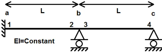
A structure can be defined as a directed graph G = (V,E) whereV is a finite vertex set of all joints and E is a finite edge set of all member ends. Consider a simple structure [West, 1989]
consisting of 3 joints (a, b, and c) and 4 ends (1, 2, 3, and 4) as shown in Figure 6.1. The initial
fixed-end moments are -172.8, 115.2, -416.7, and 416.7 kN/m, the distribution factors are 0, 0.5, 0.5, and 1, and the carryover factors are 0, 0.5, 0.5, and 0.5 for ends 1, 2, 3, and 4, respectively.
These fixed-end moments, distribution factors, and carryover factors are calculated based on the
Figure 6.1: Two Members and Three Joints Structure with Initial Fixed-End Moments
This structure can be represented by G= (V,E, f) where V ={a, b, c}and E={1,2,3,4} as shown in the Figure 6.2.
Figure 6.2: Graph Representation of Two Members and Three Joints Structure
Let function f(j, k) = ibe a one-to-one mapping function from node indexes j and k to the index of the directed edge from nodej to node k. Let function fb(i) = (j, k) be the reverse
one-to-one mapping function of f. Let function g(j, k) = (fd, fc, m) be a mapping function
from the directed edge from node j to nodek to a tuple, wherem,fd, and fc are the moment,
distribution factor, and carryover factor of the member end with indexi, respectively. In this case,
g(fb(f(a, b))) =g(fb(1)) =g(a, b) = (0,0.5,−172.8) g(fb(f(b, a))) =g(fb(2)) =g(b, a) = (0.5,0.5,115.2) g(fb(f(b, c))) =g(fb(3)) =g(b, c) = (0.5,0.5,−416.7) g(fb(f(c, b))) =g(fb(4)) =g(c, b) = (1,0.5,416.7)
6.2
Sequential Implementation
6.2.1 Flow Chart
The sequential implementation could be represented as the following flow chart.
Start
Input structure information, distribution factor,
carryover factor, and initial fixed-end moment
Is global moment distribution
converged?
Choose a subset of joints (schedule) to be released in this iteration
Record current moment distribution
and calculate unbalanced moment for all joints in the schedule
Redistribute unbalanced moment for all joints in the schedule
and add carryover moments for related adjacent joints
Output converged moment distribution
Stop yes
1 defex1():
2 a, b, c = 0, 1, 2
3 g ={a:{}, b: {}, c : {}} 4 g[a ][ b] = End(0.0, 0.5, −172.8) 5 g[b ][ a] = End(0.5, 0.5, 115.2) 6 g[b ][ c ] = End(0.5, 0.5, −416.7) 7 g[c ][ b] = End(1.0, 0.5, 416.7) 8 returng
Releasing a joint is a two-step process in order to mimic matrix multiplication where each element
is calculated independently. The first step is calculating and recording each joint’s unbalanced
moment, and the second step is to redistribute the unbalanced moment. The unbalanced moment of a joint is calculated by summing moments of member ends connecting to the joint as
1 defget unbalanced moment(g, i): 2 unbalanced moment = 0 3 for j ing[ i ]:
4 unbalanced moment += g[i][j].moment 5 returnunbalanced moment
The redistribution process distributes the unbalanced moment and carryover moments by
1 def release (g, i , unbalanced moment): 2 for j ing[ i ]:
3 my share = g[i][ j ]. distribution factor *unbalanced moment 4 g[ i ][ j ]. moment−= my share# mimic matrix D
5 g[ j ][ i ]. moment−= g[i][j].carryover factor *my share# mimic matrix CD
One iteration based on a particular schedule (a particular schedule setV(k) in Eq. 5.1) can be performed by
1 # moment distribution method with schedule 2 defmdm schedule(g, schedule, tolerance): 3 converged = True
4 unbalanced moment ={}
5 # prepare releasing a joint by calculating and recording its unbalanced moment 6 for joint inschedule:
7 if has nonzero dfs(g, joint ) :
8 unbalanced moment[joint] = get unbalanced moment(g, joint) 9 # complete releasing a joint by redistributing its unbalanced moment 10 for joint inunbalanced moment:
11 if abs(unbalanced moment[joint])>= tolerance:# stopping criteria 12 converged = False
Different from the infinite sequence of matrix multiplication in theory, the above function
mdm schedule includes a stopping criteria for practicality. In fact, a computer has limited precision for floating point numbers, which means it is almost impossible to perfectly and
accurately calculate and store the infinite sequence. Moreover, it is very rare that an engineering
project requires a large number of significant digits. Thus, in order to get an acceptable result within a reasonable time, a tolerance is necessary. The program terminates when the desired
convergence is achieved.
Since only non-fixed joints are released, the function
1 defhas nonzero dfs(g, i ) : 2 for j ing[ i ]:
3 if g[ i ][ j ]. distribution factor >0:
4 returnTrue
5 returnFalse
could be used to determine whether a joint is fixed.
The above Python code snippets actually implicitly achieve the same effect as the matrix
multiplication in Eq. 5.1 by mimicking the matrix E that includes D and CD. Because the unbalanced moment used in the lines
1 my share = g[i][ j ]. distribution factor *unbalanced moment 2 g[ i ][ j ]. moment−= my share# mimic matrix D
is calculated by summing all moments of member ends connecting to the end, multiplying this unbalanced moment by the corresponding distribution factor is exactly the same as multiplying
a row of D. Similarly,
1 g[ j ][ i ]. moment−= g[i][j].carryover factor *my share# mimic matrix CD
is exactly the same as multiplying a row ofCD by the moment vectorM. Moreover, unbalanced moments of all joints in the current schedule are calculated before any distribution process, so the second step is independent for each joint. Thus by executing release(g, i, moment) and
mdm schedule(g, schedule, tolerance), the matrix multiplication in Eq. 5.1 is implicitly performed for one iteration.
The sequential implementation repeats the above processes until global convergence is
1 # moment distribution method with simultaneous joint balancing and Jacobi schedule 2 defmdm simultaneous(g, tolerance):
3 n = 0 # number of iterations performed 4 converged = False
5 while notconverged:
6 converged = mdm schedule(g, g, tolerance)
7 n += 1
8 returnn 9
10 # moment distribution method with consecutive joint balancing and Gauss−Seidel schedule 11 defmdm consecutive(g, tolerance):
12 n = 0 # number of iterations performed 13 converged = False
14 while notconverged: 15 for i ing: 16 schedule ={i}
17 converged = mdm schedule(g, schedule, tolerance)
18 n += 1
19 returnn
Since the schedule used in mdm schedule(g, schedule, tolerance) corresponds to the schedule setV(k) in Eq. 5.1, according to Theorem 2, this implementation always generates the same solution (within tolerance) as long as all joints are included in the schedule infinitely often.
6.2.3 Example
To illustrate, consider the same structure as shown in Chapter 3. Its matrix representations are
E = Eab +Ebb+Ecb
=
0 0 0 0
0 0 0 0
0 0 0 0
0 0 0 0
+
0 -0.25 -0.25 0
0 -0.5 -0.5 0
0 -0.5 -0.5 0
0 -0.25 -0.25 0
+
0 0 0 0
0 0 0 0
0 0 0 -0.5
0 0 0 -1
(6.1)
where elements in bold are obtained from matrix E. The initial moments are
M(0) =
mab mba mbc mcb =
−172.8 115.2 −416.7
416.7
. (6.2)
form is
M1 = (I+Ebb)M(0) =
−97.4 266.0 −266.0
492.1
. (6.3)
On the other hand, the computational implementation first calculates the unbalanced moment of joint b, which is
g[b][a].moment+g[b][b].moment+g[b][c].moment= 115.2 + 0−416.7 =−301.5 , (6.4)
in functions get unbalanced moment(g, i)by the lines
1 defget unbalanced moment(g, i): 2 unbalanced moment = 0 3 for j ing[ i ]:
4 unbalanced moment += g[i][j].moment 5 returnunbalanced moment
This unbalanced moment is then compared against the tolerance in mdm schedule(g, sched-ule, tolerance)by the line
1 if abs(unbalanced moment[joint])>= tolerance:# stopping criteria
If it is greater than the tolerance, functionrelease(g, i, moment) distributes this unbalanced moment to endsbaand bc, as well as calculate and record carryover moments for endsab and
cb. Because a dictionary data structure is used, the order of these updates is indeterminate, but the result is the same. Particularly, the function
1 def release (g, i , unbalanced moment): 2 for j ing[ i ]:
3 my share = g[i][ j ]. distribution factor *unbalanced moment 4 g[ i ][ j ]. moment−= my share# mimic matrix D
5 g[ j ][ i ]. moment−= g[i][j].carryover factor *my share# mimic matrix CD
first calculates
expressed in matrix form as
M1=
mab+ 75.4 mba+ 150.8
mbc+ 150.8 mcb+ 75.4
=
−172.8 + 75.4 115.2 + 150.8 −416.7 + 150.8
416.7 + 75.4
=
−97.4 266.0 −266.0
492.1
. (6.6)
6.3
Asynchronous Shared Memory Parallel Implementation
with Simple Termination
This section describes an asynchronous shared memory parallel implementation of the method that terminates after a period of time, with the assumption that global convergence is achieved
by then.
6.3.1 Flow Chart
This asynchronous shared memory parallel implementation could be represented as the following
flow chart.
Start
Input structure information, distribution factor,
carryover factor, and initial fixed-end moment
Create thread pool (one thread per non-fixed joint)
Thread 1 Process
Thread 2 Process
. . . Thread n
Process
Join all threads
The flow chart for the each thread process is
Start thread
Is time limit exceeded?
Record current moment distribution and calculate unbalanced moment for this joint
Is this joint’s moment distribution
converged?
Redistribute unbalanced moment for this joint,
add carryover moments for related adjacent joints and nofity their threads
Stop thread
Wait until get notified
by another thread
or time limit exceeded yes
no
no
yes
6.3.2 Python Code Snippets
For asynchronous shared memory parallel implementation, exactly one thread will be created for each non-fixed joint. The following function creates and starts these threads. The program
exits after a predefined amount of time.
4 if has nonzero dfs(g, i ) : 5 print(’Starting ’ , i )
6 t = Thread(target=joint thread, args=(g, cond, i, tolerance)) 7 t .daemon = True# make thread die when main thread completes 8 t . start ()
9 sleep (1) # simple timed termination: keep main thread alive until processes are (assumed to be) ,→ done
The process of each thread is
1 # define a concurrent process for each joint i 2 defjoint thread (g, cond, i , tolerance) : 3 while True:
4 with cond[i ]: # require condition for wait/ notification in Python 5 unbalanced moment = get unbalanced moment(g, i)
6 while abs(unbalanced moment)<tolerance:# local stopping criteria
7 cond[i ]. wait()
8 unbalanced moment = get unbalanced moment(g, i) 9 release (g, cond, i , unbalanced moment)
The statement
1 moment = get unbalanced moment(g, i)
takes a snapshot of the current member end moments, which will be used to create elementary
operations.
Each thread keeps executing a slightly different release function compared to the one in sequential implementation until a global converge is achieved.
1 def release (g, cond, i , unbalanced moment): 2 for j ing[ i ]:
3 my share = g[i][ j ]. distribution factor *unbalanced moment 4 g[ i ][ j ]. decr moment(my share)# mimic matrix D, atomic
5 g[ j ][ i ]. decr moment(g[i][j ]. carryover factor * my share)# mimic matrix CD, atomic 6 with cond[j ]: # notify neighboring joint that it may now have an unbalanced moment 7 cond[j ]. notify ()
Since there is no synchronization between all threads, some threads could run faster than
others. In fact, the statement
1 g[ i ][ j ]. decr moment(my share)# mimic matrix D, atomic
exactly executes the elementary operation [i, i], and the statement
1 g[ j ][ i ]. decr moment(g[i][j ]. carryover factor * my share)# mimic matrix CD, atomic
exactly executes the elementary operation [j, i]. Moreover, a thread must finish the loop
1 for j in g[ i ]:
before starting another one, which grantees that the increments within a particular joint will
be added toMbefore releasing the same joint again. Thus, this asynchronous shared memory parallel implementation always provides same solution as the one in the sequential version
(within tolerance) according to Theorem 2.
6.3.3 Example
To illustrate, consider the same structure as shown in Chapter 3 again. According to Eq. 5.16,
the matrixE can be further decomposed in two dimensions as
E = [a, a] + [b, a] + [c, a] + [a, b] + [b, b] + [c, b] + [a, c] + [b, c] + [c, c] (6.7)
where
[a, a] =
0 0 0 0
0 0 0 0
0 0 0 0
0 0 0 0
(6.8)
[b, a] =
0 0 0 0
0 0 0 0
0 0 0 0
0 0 0 0
(6.9)
[c, a] =
0 0 0 0
0 0 0 0
0 0 0 0
0 0 0 0