Simultaneous Estimation of Mixing Rates and Genetic Drift Under Successive Sampling of Genetic Markers With Application to the Mud Crab (Scylla paramamosain) in Japan

DOI: 10.1534/genetics.106.056424

Simultaneous Estimation of Mixing Rates and Genetic Drift Under

Successive Sampling of Genetic Markers With Application to the

Mud Crab (

Scylla paramamosain

) in Japan

Toshihide Kitakado,*

,1

_{Shuichi Kitada,* Yasuhiro Obata}

†

_{and Hirohisa Kishino}

‡

*Faculty of Marine Science, Tokyo University of Marine Science and Technology, Minato, Tokyo 108-8477, Japan,†Tamano Station, National Center for Stock Enhancement, Fisheries Research Agency, Chikko, Tamano, Okayama 706-0002, Japan and‡Graduate School of

Agriculture and Life Sciences, University of Tokyo, Bunkyo, Tokyo 113-8657, Japan Manuscript received February 1, 2006

Accepted for publication June 8, 2006

ABSTRACT

In stock enhancement programs, it is important to assess mixing rates of released individuals in stocks. For this purpose, genetic stock identification has been applied. The allele frequencies in a composite population are expressed as a mixture of the allele frequencies in the natural and released populations. The estimation of mixing rates is possible, under successive sampling from the composite population, on the basis of temporal changes in allele frequencies. The allele frequencies in the natural population may be estimated from those of the composite population in the preceding year. However, it should be noted that these frequencies can vary between generations due to genetic drift. In this article, we develop a new method for simultaneous estimation of mixing rates and genetic drift in a stock enhancement program. Numerical simulation shows that our procedure estimates the mixing rate with little bias. Although the genetic drift is underestimated when the amount of information is small, reduction of the bias is possible by analyzing multiple unlinked loci. The method was applied to real data on mud crab stocking, and the result showed a yearly variation in the mixing rate.

I

T is well known that many fisheries stocks have been reduced because of overfishing, habitat loss, and degradation. (Pauly et al. 2002). Some management procedures, such as setting a total allowable catch (TAC), are the usual practices for sustainable use of such fisheries stocks (e.g., Hilbornand Walters1992). In ad-dition to such management procedures, stock enhance-ment programs through release of hatchery-reared juveniles are used to supplement reduced natural stocks (Blaxter2000; Sva˚ sandet al.2000; Leberet al. 2004; Kitadaand Kishino2006).

In stock enhancement programs, the assessment of the contribution of the released population to the commercial catch is one of the important tasks (Kitada and Kishino 2006). Also, it is necessary to monitor the genetic impact of release on a natural population. Evaluation of the mixing conditions of a released popu-lation into a natural popupopu-lation must then be carried out. However, if juveniles are too small to tag and/or the tag-shedding rate is significant, it is difficult to de-termine their mixing compositions through experi-ments with artificial tags. For such cases, there is the possibility of stock identification using genetic tags such as mtDNA haplotypes and microsatellite alleles (e.g., Leberet al.2004).

We now consider a fisheries stock of a random-mating population in a closed fishing ground. Here, we call this population a natural population. Suppose that in each year hatchery-reared juveniles are released before the fishing season. Then, a population after the release of the juveniles composes a composite population, which consists of two source populations, that is, the natural and supplemented populations. The composite popu-lation could in turn be naturally reproducing in the next year. We call it a natural population again.

The haplotype or allele frequencies in a population in the fishing ground change temporally for two reasons: the release of juveniles and the genetic drift. The amount of genetic drift depends on the effective population size (Ne) (Nei and Tajima 1981; Waples 1989). The methods for estimating Neon the basis of

temporal changes in haplotype or allele frequencies have been developed. Waples (1989) introduced a moment-based estimation method using the standard-ized variance in allele frequency change. More efficient estimation by the maximum-likelihood method was introduced by Williamson and Slatkin (1999) and Anderson et al. (2000). Furthermore, Anderson (2005) presented a coalescent-based likelihood method for temporally sampled individuals.

Such temporal change in sampled haplotype or allele frequencies can also be used for the estimation of mixing rates. Typically, the estimation of mixing rates in a mixed population needs samples from different 1_{Corresponding author:Tokyo University of Marine Science and}

Tech-nology, 5-7, Konan 4, Minato-ku, Tokyo, 108-8477, Japan. E-mail: [email protected]

baseline populations as well as the composite popula-tion. For such situations, the maximum-likelihood (ML) and Bayesian methods were developed (e.g., Millar 1987; Pella and Masuda 2001). Another situation occurs in stock enhancement programs. In this case, one baseline population is a natural population before release, and the other is a released population. A mixed population is a composite population after release. Usually, sampling from the composite population is conducted in the fishing season, and the composite population in the previous year acts as a baseline. In this sense, a composite population in one year plays two roles: as a mixed population for the sampling year and as a baseline natural population for the following year. This kind of method was applied to data for the mud crab, Scylla paramamosain, in Japan. Imai et al. (2002) used the mitochondrial DNA (mtDNA) D-loop region as a genetic tag and gave a point estimate for the mixing rate of juveniles released for a year. Obataet al.(2006) obtained point estimates of mixing rates and their confidence intervals using the maximum-likelihood method.

As mentioned above, haplotype or allele frequencies can vary due to genetic drift. Hatchery releases could be effective for depleted populations with limited recruit-ment. Supportive breeding (Rymanand Laikre1991) programs also target small populations of endangered species. In such cases, the effective population size could be small and the amount of genetic drift cannot be ignored. If the effect of genetic drift is large, actual haplotype or allele frequencies in the natural popula-tion, regarded as a baseline populapopula-tion, are different from frequencies in the natural population at release. The natural population at release should actually act as a baseline. Obataet al.(2006) conducted a simulation for sensitivity tests to quantify the magnitude of changes in estimates and standard errors of mixing rates for various values of genetic drift assumed to be known. However, the effect of the genetic drift on the estimate of the mixing rate has not been fully evaluated and the reliability of the classical method for such situations remains unknown.

In this article, we develop a new method to simulta-neously estimate mixing rates and the magnitude of the genetic drift, on the basis of successive allelic frequen-cies. Our statistical model includes further parameters such as frequencies in the initial population and latent vectors that represent random haplotype or allele fre-quencies due to genetic drift. While the complete likelihood function for such latent variables and ob-served data can be explicitly expressed, the likelihood function for observed data does not have a closed form. To obtain the maximum-likelihood estimate of the genetic drift, we use a Monte Carlo approximation of likelihood with a Markov chain Monte Carlo (MCMC) method (e.g., Gelmanet al.2004; Robertand Casella 2004). Performance of the proposed method was

evaluated via numerical simulations and real data of mud crab stocking in Japan were analyzed.

MODELS AND METHODS

We mostly illustrate our statistical model and estima-tion method for the case where alleles at a single locus (or haplotypes in mtDNA) are observed.

Statistical model: Let p1y¼ ðp1y1;. . .;p1yJÞ be a

vector of the true allele frequencies for a population in a fishing ground in year yðy¼1;2;. . .;YÞ, where J is the number of alleles and PJ_j¼1p1yj¼1. Let

n1y¼ ðn1y1;. . .;n1yJÞ denote the observed allele

fre-quencies of samples randomly collected from this nat-ural population in yeary. Then, givenp1y, the observed

frequencies n1y are assumed to have a multinomial

distribution,

fðn1yjp1yÞ ¼ N1y!

QJ j¼1n1yj!

YJ

j¼1 pn1yj

1yj ðy¼1;2;. . .;YÞ;

where N1y¼

PJ

j¼1n1yj is twice the sample size for the

diploid (the sample size itself for the haploid marker). Suppose that juveniles are reared each year using some sampled individuals with minor alleles and then released into the natural population in the following year. In this case, the alleles used in the released population act as genetic tags in the natural population. Letp2y ¼ ðp2y1;. . .;p2yJÞbe a vector of allele

frequen-cies for released juveniles in year yðy¼2;3;. . . ;YÞ

(PJ_j¼1p2yj ¼1). Let n2y¼ ðn2y1;. . .;n2yJÞdenote

sam-pled counts of allele frequencies from the released population in yearywith a multinomial distribution,

fðn2yjp2yÞ ¼ N2y!

QJ j¼1n2yj!

YJ

j¼1 pn2yj

2yj ðy¼2;3;. . .;YÞ;

whereN2y ¼

PJ j¼1n2yj.

The allele frequencies in the population in the fishing ground change due to two factors: genetic drift and the release of juveniles into the population. To rep-resent the variation due to the genetic drift, we assume a Dirichlet distribution with a probability density function

pð˜p1y;p1;y1;uÞ ¼

GðuÞ

QJl

j¼1Gðup1;y1;jÞ

YJ

j¼1

˜pup1;y1;j1

1yj

ðy¼2;3;. . .;YÞ; ð1Þ

where˜p1yis a vector of allele frequencies before release

frequency in the previous generation and Ne is the

effective population size (e.g., Nei and Tajima 1981; Waples 1989). Note that the variance for mtDNA haplotype frequencies isp(1 p)/Nf, whereNfis the

effective female population size. In this model, the variance of˜p1ybased on the Dirichlet distribution above

is given by

Var½˜p1yj ¼ 1

11up1;y1;jð1p1;y1;jÞ:

Hence, the parameteruis closely related to the effective population size as 11u ¼2Neor 11 u ¼Nf. In this

article, we assume a constantuover all years.

Now, the vector of frequencies˜p1ycannot be observed

because the sample is taken after the release of juveniles, and therefore it is regarded as a latent random vector. After the genetic drift among years, the vector of allele frequencies further changes because of mixing with the released juveniles, as

p1y¼ ð1vyÞ˜p1y1vyp2y ðy¼2;3;. . .;YÞ;

wherev_yis the mixing rate of the released population into the natural population in yeary. As a summary of our statistical model, a schematic diagram is shown in Figure 1.

Likelihood: In this model, unknown parameters are

mixing rates,v¼ ðv2;v3;. . .;vYÞ, the degree of the

genetic drift,u, the vector of the true allele frequencies in a natural population in the initial year,p11, and those

of the released population, p2yðy¼2;. . . ;YÞ. For

notational convenience, we summarize random varia-bles as n1¼ fn1y;y¼1;2;. . .;Yg, n2 ¼ fn2y;y¼

2;. . .;Yg, ˜p1 ¼ f˜p1y;y¼2;3;. . .;Yg, and p2¼

ðp22;. . .;p2YÞ. If the latent vectors˜p1 can be observed,

the likelihood function for the unknown parameters,v,

u,p11,p2, based on the observationsn1,n2and the latent

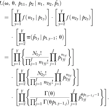
variables˜p1, is explicitly expressed as follows:

Lðv;u;p11;p2jn1;n2;˜p1Þ

¼ Y

Y

y¼1

fðn1yjp1yÞ

" #

Y

Y

y¼2

fðn2yjp2yÞ

" #

Y

Y

y¼2

pð˜p1yjp1;y1;uÞ

" #

¼ Y

Y

y¼1

N1y!

QJ j¼1n1yj!

YJ

j¼1 pn1yj

1yj

( )

" #

Y

Y

y¼2

N2y!

QJ j¼1n2yj!

YJ

j¼1 p2nyj2yj

( )

" #

Y

Y

y¼2

GðuÞ

QJ

j¼1Gðup1;y1;jÞ

YJ

j¼1

˜pup1;y1;j1

1yj

( )

" #

:

Now, ˜p1are unobservable latent variables, and hence

we must consider a likelihood function based on the marginal distribution ofn1andn2as follows:

LMðv; u;p11;p2jn1;n2Þ

¼

ð

. . .

ð

Lðv;u; p11;p2jn1;n2;˜p1Þd ˜p12 . . .d ˜p1Y:

Unfortunately, an explicit formula for the marginal likelihood function is not available. To find the max-imum-likelihood estimates, we use a Monte Carlo approximation of likelihood as explained below.

Estimation algorithm: For simplicity of illustration,

we assume that the allele frequenciesp2are known. In

this case, the observationn2is not used in the

estima-tion. The method with unknownp2is straightforward.

Let f denote the set of parameters (v, u, p11). To

approximate LM(fjn1) via a Monte Carlo simulation,

we use the formula

LMðfjn1Þ LMðf*jn1Þ

¼

ð

. . .

ð

Lðfjn1;˜p1Þ Lðf*jn1;˜p1Þ

pð˜p1jn1;f*Þd ˜p12. . .d ˜p1Y;

where f* is a reference vector, andpð˜p1jn1;f*Þis the

conditional distribution of the latent variables˜p1atf*

given the observed data n1. This integration can be

approximated by Monte Carlo as

LMðfjn1Þ

LMðf*jn1Þ

1 m

Xm

i¼1

Lðfjn1;˜pðiÞ₁ Þ

Lðf*jn1;˜pðiÞ1 Þ

;

where˜pð1Þ 1 ;. . .;˜p

ðmÞ

1 are the realization of˜p1drawn from

the conditional distributionpð˜p1jn1;f*Þ.

Unfortunately, a closed form of the conditional dis-tributionpð˜p1jn1;f*Þdoes not exist because it includes

the marginal distributionLM(f*jn1). To generate the

ran-dom numbers frompð˜p1jn1;f*Þ, we use a

Metropolis-within-Gibbs sampling method (e.g., Robert and Casella2004). Details of this algorithm are described inappendix a.

Figure1.—A schematic of the statistical model with genetic

In general, the precision of the approximation de-pends on the choice off* as well as the size ofm. One option for the determination ofv* andp*₁₁inf* is to use the maximum-likelihood estimates by ignoring the genetic drift. In this case, no latent variables are in-cluded in the likelihood. Another option is to use a Monte Carlo version of the EM algorithm (e.g., McLachlan and Krishnan 1997). A detailed description of this algorithm is given in appendix b. It is known that convergence of the EM algorithm tends to be slow, but values of parameters that are innovated up to several steps can be used forf*, includingu*.

The case of multiple unlinked loci: Our model can

be extended for the case of multiple unlinked loci by considering the composite genotype frequencies. Dif-ferent loci receive independent genetic drifts, and therefore the distribution of the latent allele frequen-cies, which is expressed in Equation 1, can be defined locus-by-locus. On the other hand, although the com-posite genotype frequencies are expressed as products of the genotype frequencies at the loci, the probability distribution of observed composite genotype is not given by the product of multinomial distributions for the loci. Here, we denote byx1yila composite genotype

at thelth locus for theith individual sampled from the composite population in yeary(2#y#Y) and by˜p1yl

andp2ylvectors of allele frequencies at thelth locus in

the natural population before release and in the re-leased population in year y, respectively. Then the distribution ofx1yigiven˜p1yl andp2ylis expressed as

ð1vyÞ

YL

l¼1

fðx1yilj˜p1ylÞ1vy

YL

l¼1

fðx1yiljp2ylÞ;

whereLis the number of loci, and thef’s are probability distributions for the two source populations. The esti-mation algorithm with a MCMC becomes complicated for this case because the acceptance ratios in MCMC samplings depend on information from all the loci. In this article, we use the product of multinomial distribu-tions from each locus as an approximated model.

SIMULATION STUDIES

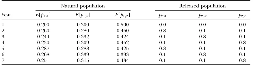
Simulation scenarios: To evaluate the estimation

performance in our statistical model and the difference of estimates between considering and ignoring the genetic drift, we used simulation studies. As scenario I, the length of sampling years was fixed at 7, and the number of loci was assumed to be 1 or 5. Furthermore, as scenario II, we considered an extreme case where samples were taken for only 2 years. In this scenario, 5 or 10 loci were analyzed to cover the limited information from only 2 years. The allele frequencies in the natural population in the initial year and those in released populations were assumed to be common over loci, and the frequencies in the released populations were known. Note that, for the case of multiple loci, com-posite genotypes were generated from the true distri-bution, and then parameters were estimated using the approximated likelihood. To make the computational time shorter, we assumed a case of only three alleles. The mixing rates, of 0.1, were assumed to be the same over the years. Three levels of genetic drift,u¼10, 100, and 1000, were used. The same sample size,Ny¼500, was

assumed each year. Scenarios we used in this simulation are summarized in Table 1. The frequencies in the released populations are assumed to be known. Throughout this simulation study, we set the true values of parameters for f*. Considering the computational burden, the sample size of the MCMC was fixed at 5000. Among 5000 samples, the first 1000 samples were discarded as constituting the burn-in period, and every fifth simulation draw was kept. Therefore, the effective sample size was 800. The number of simulation replicas was 100 for each scenario. All the computation was carried out using our own program written by statistical software R (http://www.r-project.org/).

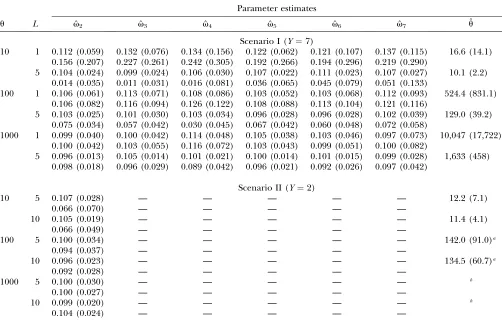
Simulation results:The results are shown in Table 2.

In scenario I (Y¼7), although the estimate ofutended to be overestimated, especially for the case ofL¼1 and larger values ofu, estimates of the mixing rates,v’s, by the model that considered the genetic drift were almost unbiased throughout the simulation. The bias of ˆuwas

TABLE 1

True allele frequencies used in simulation studies

Natural population Released population

Year E[p1y1] E[p1y2] E[p1y3] p2y1 p2y2 p2y3

1 0.200 0.300 0.500 0.0 0.0 0.0

2 0.260 0.280 0.460 0.8 0.1 0.1

3 0.244 0.332 0.424 0.1 0.8 0.1

4 0.230 0.309 0.462 0.1 0.1 0.8

5 0.287 0.288 0.425 0.8 0.1 0.1

6 0.268 0.339 0.393 0.1 0.8 0.1

7 0.251 0.315 0.434 0.1 0.1 0.8

The mean of allele frequencyE[p1yj] was calculated using the recursive formula.E½p1yj ¼ ð1vyÞE½p1;y1;j1

reduced when multiple loci (L¼5) were analyzed. On the contrary, those where the genetic drift was not considered were subject to large bias whenuwas small; that is, the degree of genetic drift was large. Note that the estimation performance for the mixing rates tended to be similar in both the models foru¼1000, the case of small genetic drift.

In scenario II (Y ¼ 2), because of the small size of replication with respect to years, the estimation was more difficult to make than in scenario I. In fact, especially for the case ofu¼1000, the estimates ofutend to be infinity. Hence, we set an upper bound, 5000, for the estimate ofu. However, the simulation results suggest that the estima-tion ofuwith many loci performs well when genetic drift is large. The estimation on mixing rates while considering the genetic drift was also stable in this scenario. On the other hand, biases were observed in the estimates without considering the drift. A noteworthy fact is that the biases are smaller than those in scenario I, where samples were taken for $7 years than the 2 in scenario II. This

phenomenon indicates that the large bias in scenario I was due to the impact of the genetic drift through the year. Therefore, the longer the sampling period is the more effective it is to take the genetic drift into account.

To reduce the computation time for the simulation, we assumed only three alleles in our simulation studies. The allele or haplotype frequencies in the released population have a large impact on the estimation of mixing rates rather than the number of alleles. The results for our model with considering genetic drift showed that the estimation performance of mixing rates in years 4 and 7 for scenario I tended to be worse than that in other years. This is because the most common allele in the released population is also most common in the natural population before release. On the other hand, smaller standard deviations were observed in years 2 and 5, when the common allele in the released population is a rare allele in the natural population. In this way, use of rare alleles or haplotypes for the released population improves the estimation performance.

TABLE 2

Expectations of estimators for mixing rates and genetic drift

Parameter estimates

u L vˆ2 vˆ3 vˆ4 vˆ5 vˆ6 vˆ7 uˆ

Scenario I (Y¼7)

10 1 0.112 (0.059) 0.132 (0.076) 0.134 (0.156) 0.122 (0.062) 0.121 (0.107) 0.137 (0.115) 16.6 (14.1) 0.156 (0.207) 0.227 (0.261) 0.242 (0.305) 0.192 (0.266) 0.194 (0.296) 0.219 (0.290)

5 0.104 (0.024) 0.099 (0.024) 0.106 (0.030) 0.107 (0.022) 0.111 (0.023) 0.107 (0.027) 10.1 (2.2) 0.014 (0.035) 0.011 (0.031) 0.016 (0.081) 0.036 (0.065) 0.045 (0.079) 0.051 (0.133)

100 1 0.106 (0.061) 0.113 (0.071) 0.108 (0.086) 0.103 (0.052) 0.103 (0.068) 0.112 (0.093) 524.4 (831.1) 0.106 (0.082) 0.116 (0.094) 0.126 (0.122) 0.108 (0.088) 0.113 (0.104) 0.121 (0.116)

5 0.103 (0.025) 0.101 (0.030) 0.103 (0.034) 0.096 (0.028) 0.096 (0.028) 0.102 (0.039) 129.0 (39.2) 0.075 (0.034) 0.057 (0.042) 0.030 (0.045) 0.067 (0.042) 0.060 (0.048) 0.072 (0.058)

1000 1 0.099 (0.040) 0.100 (0.042) 0.114 (0.048) 0.105 (0.038) 0.103 (0.046) 0.097 (0.073) 10,047 (17,722) 0.100 (0.042) 0.103 (0.055) 0.116 (0.072) 0.103 (0.043) 0.099 (0.051) 0.100 (0.082)

5 0.096 (0.013) 0.105 (0.014) 0.101 (0.021) 0.100 (0.014) 0.101 (0.015) 0.099 (0.028) 1,633 (458) 0.098 (0.018) 0.096 (0.029) 0.089 (0.042) 0.096 (0.021) 0.092 (0.026) 0.097 (0.042)

Scenario II (Y¼2)

10 5 0.107 (0.028) — — — — — 12.2 (7.1)

0.066 (0.070) — — — — —

10 0.105 (0.019) — — — — — 11.4 (4.1)

0.066 (0.049) — — — — —

100 5 0.100 (0.034) — — — — — 142.0 (91.0)a

0.094 (0.037) — — — — —

10 0.096 (0.023) — — — — — 134.5 (60.7)a

0.092 (0.028) — — — — —

1000 5 0.100 (0.030) — — — — — b

0.100 (0.027) — — — — —

10 0.099 (0.020) — — — — — b

0.104 (0.024) — — — — —

Values in the top and bottom rows in each case showed the results of the models with and without considering genetic drift, respectively. The values in parentheses are standard deviations. The true mixing rates were assumed to be 0.1. The sample size was fixed at 500 through all years. In scenario II, an upper bound for the estimate ofuwas set at 5000.

a_{The estimates ofuthat attained the upper bound (36 and 27 times forL¼5 and 10, respectively) were excluded from the} calculation of the mean and standard deviation.

b

CASE STUDY: ANALYSIS FOR MUD CRABS

Data: In Japan, three mud crab species, S.

para-mamosain, S. serrata, and S. olivacea, are commercially important resources in local scale fisheries. Urado Bay in Kochi Prefecture is the main area forS. paramamosain fisheries. The life span of this crab is from 1.5 to 2.5 years (Obata et al. 2006). May and June are the spawning season, and in September hatched crabs grow to commercial size and recruit into the fishing ground. The fishery is operated mainly from August to December with the highest catch in September. The commercial catch of this species has fallen since the mid-1970s from

12 tons and reached a record low of 1.6 tons in 1989. In the early 1980s, a stock enhancement program for this species started in Urado Bay, and the number of released juveniles has increased.

To examine the efficacy of the release program for this species, an experiment using genetic tagging was conducted (Obataet al.2006). Samples were collected in Urado Bay around December in 1996–2002. In each year from 1996 to 2000, individuals with different haplotypes were chosen from samples to produce supplemental juveniles, and these minor haplotypes would then be used as a genetic tag. During mid-May/ early June in each of the next years, juveniles were released into Urado Bay. Supplemented individuals, if not removed by fishing from the population in the year they are introduced, can contribute to the reproducing population in the second year.

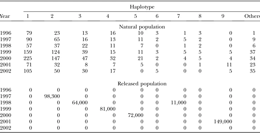
We used observed haplotype frequencies in the mtDNA D-loop region of the mud crabs (Table 3). Here, we grouped very minor haplotypes into one category called ‘‘others.’’ The haplotype frequencies

for the released population are also shown in Table 3. Only one haplotype was released every year, except 1998. Using these data, we estimated mixing rates and the genetic drift simultaneously. Because the number of released juveniles was known, we can regard the parameters p2y as fixed. We set the burn-in period at

5000 and kept every fifth simulation draw of 250,000 samples as an effective output for Monte Carlo sampling.

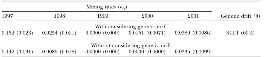
Results: Table 4 shows the summary of parameter

estimations with and without taking the genetic drift into account. The estimates of mixing rates, ˆvy, were

small except for 1997. Little differences between the estimates of the two methods were observed. This may be due to the small genetic drift. In fact, the estimatedu

was341.1. Althoughu may be overestimated consid-ering the simulation results, severe genetic drift was not observed.

Although not so much difference in the number of released juveniles was recorded except for in 2001, a large yearly variation in the estimates of mixing rates was observed. In the next section, we discuss the effects of adaptation and selection on the estimation of mixing rates.

DISCUSSION

In this article, we proposed a statistical model for the simultaneous estimation of mixing rates and genetic drift for stock enhancement programs. In our model, temporal changes in haplotype or allele frequencies are modeled, taking into account mixing and genetic drift. This model can be regarded as an extension of work by

TABLE 3

A summary of observed haplotype frequencies in the mtDNA D-loop region ofS. paramamosainfor the

natural and the released populations

Haplotype

Year 1 2 3 4 5 6 7 8 9 Others

Natural population

1996 79 23 13 16 10 3 1 3 0 1

1997 90 65 16 13 11 2 5 2 0 9

1998 57 37 22 11 7 0 1 2 0 6

1999 159 124 39 15 11 3 5 5 5 37

2000 225 147 47 32 21 2 4 5 4 34

2001 71 32 8 7 5 0 0 1 11 23

2002 105 50 30 17 0 5 0 0 5 35

Released population

1996 0 0 0 0 0 0 0 0 0 0

1997 0 98,300 0 0 0 0 0 0 0 0

1998 0 0 64,000 0 0 0 11,000 0 0 0

1999 0 0 0 81,000 0 0 0 0 0 0

2000 0 0 0 0 72,000 0 0 0 0 0

2001 0 0 0 0 0 0 0 0 149,000 0

Andersonet al.(2000), in which temporal changes due to genetic drift only were assumed and the effective population size (Ne) was estimated using the

relation-ship between the genetic drift andNe. Our simulation

studies demonstrated that the performance for the estimation of the mixing rates, v, based on the pro-posed model, was much better than that based on the model ignoring the genetic drift if the degree of genetic drift was large. Also, even if the degree of genetic drift was small, the mixing rates were well estimated.

Meanwhile, the simulation results also showed that the estimation of genetic drift is difficult compared to that of mixing rates. The genetic drift u was over-estimated especially when the genetic drift was small. In fact, the standard errors foruin the case studies for mud crabs were large. This is partly due to the small number of sampling years and partly due to the use of only the mtDNA haplotype frequencies. Longer-term research would improve the estimation performance for the genetic drift and the mixing rates. In such studies, however, we must also consider the change inu

orNethrough time, because the parameteruis closely

related to the effective population size. Such variation may be likely in situations where juveniles are artificially released. Note that our model does not take into account effects of removal of individuals. We supposed that individuals are randomly caught by fisheries from the composite populations, and therefore change in haplotype frequencies due to fisheries catch occurs in the same manner as the genetic drift. In this respect, we think that any changes in statistical model are not essentially necessary even if considering the effect. However, we regarded such random changes as only a result of genetic drift and related it to the effective population size. If the amount of sample is large, effective population size after the fishing season may be underestimated.

The estimates ofufor mud crabs in Urado Bay were 341.1. Because mtDNA haplotypes were used in the analysis here, the degree of genetic driftuis equal to the effective female population size minus one,Nf1. If

the sex ratio is 1:1, then the estimate of the effective population size is Ne ¼ 2Nf ¼ 684.2. Although the

accuracy of this value is not high because of the large standard error foru, it seems to be small compared to the actual population size. The catch, in weight, in the late 1990s was 5 tons, and the average weight was estimated as 411 g through a market survey (Obataet al. 2006). Hence, the catch in number can be calculated at 12,165. The mortality rate is unknown for this stock, but if the exploitation rate can be assumed to be 33% and the natural mortality is ignored, the actual population size after exploitation,N, is (10.33)5000/(0.411

0.33) 24,700. This value is considerably larger than the estimatedNe. However, as described in Turneret al.

(2002), the estimate of the ratioNe/Nfor the red drum,

Sciaenops ocellatus, was,0.001. The ratioNe/Ncan take

small values in nature, for example, if heterogeneity in fecundity or reproductivity among individuals or habitat is large. In this case, genetic impacts of hatchery releases on wild populations cannot be ignored. In this regard, further studies are necessary for the investigation ofNe

and mixing for mud crabs in Urado Bay.

Our statistical model does not take into account selection on the juvenile mortality and fertility. For our situation, there are two possible selection forces: domestication and natural selection. Domestication is defined as genetic changes that result from different selective pressures in the hatchery and the wild envi-ronment (Waples and Drake 2004). If a hatchery population was established from the natural population and then kept in the hatchery and multiplied, the hatchery-reared stock generally becomes adapted to hatchery conditions and maladapted to natural con-ditions. Therefore, the mixing rate in the fishery season can be different from the one at the time of release. Our model estimates the former. Domestication may also cause a difference in fertility between the released individuals and the others in the composite population. In addition, natural selection is another factor that has an impact on changes in haplotype frequencies. In this study, we consider only the genetic drift and ignore the difference in the fertility and fitness.

If such selection in the reproduction process is mild and the effective population size is small, the effect on the estimation of mixing rates may be small. Meanwhile,

TABLE 4

Summary of parameter estimations

Mixing rates (vy)

1997 1998 1999 2000 2001 Genetic drift (u)

With considering genetic drift

0.152 (0.023) 0.0254 (0.021) 0.0000 (0.000) 0.0151 (0.0071) 0.0389 (0.0086) 341.1 (69.4)

Without considering genetic drift

0.142 (0.031) 0.0085 (0.018) 0.0000 (0.000) 0.0000 (0.0000) 0.0335 (0.0099)

if the effect of selection is relatively large, the directional changes in the frequencies may cause a bias in our estimation of mixing rate. For example, assume that minor haplotype I is used for release in one year and another haplotype II is used in the next year. Suppose that fitness of haplotype I is low. In this case, the frequency of haplotype I before release in the next year decreases due to selection. Therefore, the mixing rate of the released population with haplotype II is over-estimated. If the same haplotype I is used in both years, and fitness of haplotype I stays low, then mixing rate is in turn underestimated. In this way, our estimates of mixing rates might be biased if the effect of selection is large. On the other hand, selection increases the level of genetic drift because it increases the rate of in-breeding. The result in the mud crab analysis showed a small level of genetic drift. We used wild female crabs caught in the fishing ground for juvenile production every year and duration for juveniles kept in the hatchery environment was short, 1 month or 1.5 months. Therefore, the domestication selection might be neglected for this case. Minor haplotypes are considered the consequence of long-term natural selec-tion and evoluselec-tion. Although further investigaselec-tion is necessary, it may have suggested a small impact of selection on the estimation.

In this article, we described mostly a statistical model only for cases where haplotype or allele counts at a single locus are observed. Now, many microsatellites are often used in the study of population genetics, in-cluding genetic stock identification (e.g., Wirginand Waldman2005). The extension for multiple unlinked markers is direct. Even with loosely linked markers, our statistical models may perform well. However, the effect of linkage disequilibrium can be stronger than that in usual population genetics studies.

Linkage disequilibrium exponentially decays with successive generations. Hence, in a population reaching equilibrium, the assumption of independence among loci will be appropriate. Our article, however, considers admixture of yearly released populations, and it is impossible to expect such equilibrium. Therefore, the assumption of independent loci tends to no longer hold. Statistical models under linkage disequilibrium have been developed (e.g., Falushet al. 2003; Kitada and Kishino 2004). However, we think that such modeling and developing of estimation methods them-selves are pretty complicated and beyond the scope of our research. Therefore, statistical models considering linkage disequilibrium as well as the mixing rates and genetic drift will be developed in future research.

Our statistical model included latent vectors repre-senting haplotype frequencies in mtDNA due to genetic drift. The likelihood function is not expressed in a closed form, and hence direct maximization is not possible. In this article, we consider the maximum-likelihood estimation with a Monte Carlo

approxima-tion of likelihood (and Monte Carlo EM, MCEM, algorithm). Meanwhile, the maximum-likelihood esti-mate is not always the best because the profile likelihood has a drawback when the sample size is small compared to the number of parameters (e.g., Neymanand Scott 1948). In fact, for more precise estimation of u, eliminating the other parameters includingvthrough integration may be efficient (Kitakado et al. 2006, accompanying article in this issue). In this case, some noninformative prior distributions are to be assumed, and the parameters, except for u, are integrated out from the likelihood. The parameter u is estimated by maximizing the integrated likelihood, and the param-eters, except for u, are inferred using their posterior distribution given data and the estimate ofu. This kind of hierarchical structure is also effective in a more practical situation where there is a random or systematic change in u over years. Although in this case further hierarchical modeling is necessary, extension of our model and algorithm is not difficult for such purposes. Furthermore, if we consider the presence of locus-specificu, the assumption of random variation ofuover loci could contribute to the reduction in the number of parameters as well as an improvement of estimation performance. In this case, further complicated algo-rithms would be necessary. These are matters to be investigated in future research.

In this article, we have developed a statistical method for estimating mixing rates of hatchery-released indi-viduals in enhanced populations. Such mixing could also occur when the outside species or population comes from a natural population. In this sense, we note that our method under successive sampling can also be applied in conservation genetics to monitor the effect of invasion by outside populations.

The authors are grateful to two anonymous reviewers for their valuable comments on the original version of this manuscript. We also thank Katsuyuki Hamasaki, Naohisa Kanda, and Hiroshi Okamura for their helpful comments.

LITERATURE CITED

Anderson_{, E. C., 2005 An efficient Monte Carlo method for}

esti-matingNe from temporally spaced samples using a

coalescent-based likelihood. Genetics170:955–967.

Anderson_{, E. C., E. G. W}illiamson _{and E. A. T}hompson_,

2000 Monte Carlo evaluation of the likelihood forNe from

temporally spaced samples. Genetics156:2109–2118.

Blaxter, J. H. S., 2000 The enhancement of marine fish stocks.

Adv. Mar. Biol.38:1–54.

Falush, D., M. Stephensand J. K. Pritchard, 2003 Inference of

population structure using multilocus genotype data: linked loci and correlated allele frequencies. Genetics164:1567–1587. Gelman, A., J. B. Carlin, H. S. Stern and D. B. Rubin,

2004 Bayesian Data Analysis, Ed. 2. Chapman & Hall/CRC Press, Boca Raton, FL.

Hilborn_{, R., and C. J. W}alters_{, 1992 Quantitative Fisheries Stock}

Assessment: Choice, Dynamics and Uncertainty, Chapman & Hall, New York.

Imai, H., Y. Obata, S. Sekiya, T. Shimizu and K. Numachi,

of mud crab juveniles,Scylla paramamosainin a natural popula-tion. Suisan Zoshoku50:149–156.

Kitada, S., and H. Kishino, 2004 Simultaneous detection of

link-age disequilibrium and genetic differentiation of subdivided populations. Genetics167:2003–2013.

Kitada_{, S., and H. K}ishino_{, 2006 Lessons learned from Japanese}

ma-rine finfish stock enhancement programmes. Fish. Res.80:101–112. Kitakado, T., S. Kitada, H. Kishinoand H. J. Skaug, 2006 An

integrated-likelihood method for estimating genetic differentia-tion between populadifferentia-tions. Genetics173:2073–2082.

Leber_{, K. M., S. K}itada_{and H. L. B}lankenship_{, 2004 Stock}

Enhance-ment and Sea Ranching, Ed. 2. Blackwell Publishing, Oxford. Mc_Lachlan_{, G. J., and T. K}rishnan_{, 1997 The EM Algorithm and}

Extensions.John Wiley & Sons, New York.

Millar_{, R. B., 1987 Maximum likelihood estimation of mixed stock}

fishery composition. Can. J. Fish. Aquat. Sci.44:583–590. Nei, M., and F. Tajima, 1981 Genetic drift and estimation of

effec-tive population size. Genetics98:625–640.

Neyman, J., and E. L. Scott, 1948 Consistent estimates based on

partially consistent observations. Econometrica16:1–32. Obata, Y., H. Imai, T. Kitakado, K. Hamasaki and S. Kitada,

2006 The contribution of stocked mud crabsScylla paramamo-sainto commercial catches, estimated using a genetic stock iden-tification technique in Japan. Fish. Res.80:113–121.

Pauly, D., V. Christensen, S. Gue´ nette_{, T. J. P}itcher, U. R. Sumaila

et al., 2002 Towards sustainability in world fisheries. Nature418:

689–695.

Pella, J., and M. Masuda, 2001 Bayesian methods for analysis of

stock mixtures from genetic characters. Fish. Bull.99:151–167.

Robert, C. P., and G. Casella, 2004 _{Monte Carlo Statistical Methods},

Ed. 2. Springer-Verlag, New York.

Ryman, N., and L. Laikre, 1991 Effects of supportive breeding on

the genetically effective population size. Conserv. Biol.5:325–329. Sva˚ sand_{, T., T. S. K}ristiansen, T. Pedersen, A. G. V. Salvanes, R.

Engelsen_{et al., 2000 The enhancement of cod stocks. Fish}

Fish.1:173–205.

Turner, T. F., J. P. Waresand R. G. John, 2002 Genetic effective size

is three orders of magnitude smaller than adult census size in an abundant, estuarine-dependent marine fish (Sciaenops ocellatus). Genetics162:1329–1339.

Waples, R., 1989 A generalized approach for estimating effective

size from temporal changes in allele frequency. Genetics121:

379–391.

Waples_{, R., and J. D}rake_{, 2004 Risk/benefit consideration for}

ma-rine stock enhancement: a Pacific salmon perspective, pp. 260– 306 inStock Enhancement and Sea Ranching, Ed. 2, edited by K. M. Leber, S. Kitadaand H. L. Blankenship. Blackwell Publishing,

Oxford.

Williamson_{, E. G., and M. S}latkin_{, 1999 Using maximum}

likeli-hood to estimate population size from temporal changes in allele frequencies. Genetics152:755–761.

Wirgin, I., and J. R. Waldman, 2005 Use of nuclear DNA in stock

indentification: single-copy and repetitive sequence markers, pp. 331–370 inStock Identification Methods, edited by S. X. Cadrin,

K. D. Friedland_{and J. R. W}aldman_{. Elsevier Academic Press,}

Burlington, MA.

Communicating editor: R. W. Doerge

APPENDIX A: MCMC SAMPLING

We illustrate a method for generating random numbers from pð˜p1jn1;f*Þ using a Metropolis-within-Gibbs

sampling method. Let ˜pð0Þ 1 ¼ f˜p

ð0Þ

1y;y¼2;3;. . .;Yg be the initial values for this algorithm. Then a sequence of

random vectors is generated in turn,

˜pði1211Þpð˜p12jn1; ˜p ðiÞ 13; ˜p

ðiÞ 14;. . .; ˜p

ðiÞ 1Y;f*Þ; ˜pði1311Þpð˜p13jn1; ˜p

ði11Þ 12 ; ˜p

ðiÞ 14;. . . ; ˜p

ðiÞ 1Y;f*Þ;

˜pði1Y11Þpð˜p1Yjn1; ˜p ði11Þ 12 ;. . .;˜p

ði11Þ 1;Y2; ˜p

ði11Þ

1;Y1;f*Þ: ðA1Þ

The method for actual generation is as follows:

1. Sample a candidate vector˜p1* from a proposal distributiony gð:j˜p ðiÞ 1yÞ

2. Compute acceptance ratios defined by

rð˜pð₁i_yÞ;˜p1*yÞ ¼

min fðn1yj˜p1*y;v*yÞpð˜p1*yj ð1vy*1Þ˜p

ði11Þ

1;y11v*y1p2;y1;u*Þ

fðn1yj˜p1ðiyÞ;v*yÞpð˜p

ðiÞ

1yj ð1vy*1Þ˜p

ði11Þ

1;y11vy*1p2;y1;u*Þ

pð˜p

ðiÞ

1;y11j ð1v*yÞ˜p*1y1v*yp2y;u*Þgð˜p

ðiÞ

1yj˜p1*yÞ pð˜pðiÞ

1;y11j ð1v*yÞ˜pð1iyÞ1v*yp2y;u*Þgð˜p1*yj˜p

ðiÞ

1yÞ

;1 !

fory¼2;. . .;Y1;

min fðn1yj˜p1*y;v*yÞfð˜p1*yj ð1vy*1Þ˜p

ði11Þ

1;y11v*y1p2;y1;u*Þgð˜p

ðiÞ

1yj˜p1*yÞ

fðn1yj˜pð1iyÞ;v*yÞfð˜p

ðiÞ

1yj ð1vy*1Þ˜p

ði11Þ

1;y11vy*1p2;y1;u*Þgð˜p1*yj˜pð1iyÞÞ

;1 !

fory¼Y:

8 > > > > > < > > > > > :

3. Setpð1iy11Þas

p₁ði_y11Þ¼ p1*y with probabilityrð˜p

ðiÞ 1y;p1*yÞ; p1ðiÞy otherwise:

For example, the form of the acceptance ratio is justified by the following formula:

fðn1;˜pði1211Þ;. . .;˜p ði11Þ 1;y1;˜p1*y;˜p

ðiÞ

1;y11;. . .;˜p ðiÞ 1Y;f*Þ fðn1;˜pði₁₂11Þ;. . .;˜pði₁;1y11Þ;˜p

ðiÞ 1y;˜p

ðiÞ

1;y11;. . . ;˜p ðiÞ 1Y;f*Þ

¼ fðn1yj˜p1*y;v*yÞpð˜p1*yjp

ði11Þ

1;y1;u*Þpð˜p ðiÞ

1;y11j ð1v*yÞ˜p1*y1v*p2y y;u*Þ fðn1yj˜pðiÞ1y;v*yÞpð˜pðiÞ1y jp

ði11Þ

1;y1;u*Þpð˜p ðiÞ

1;y11j ð1v*yÞ˜pðiÞ1y1v*p2y y;u*Þ

: ðA2Þ

As a proposal distribution forgð˜p1yj˜p ðiÞ

1yÞ, we use a Dirichlet distribution as

gð˜p1yj˜p ðiÞ 1yÞ ¼

GðcÞ

QJ j¼1Gðc ˜p

ðiÞ 1yjÞ

YJ

j¼1 ˜pc ˜p

ðiÞ

1yj1

1yj ;

where the parameterccontrols a deviation between a candidate vectorp1* and the previous vectory ˜p ðiÞ

1yj. In fact, the variance

of ˜p1* is given byy ˜p ðiÞ 1yjð1˜p

ðiÞ

1yjÞ=ð11cÞ, and therefore the mixing condition over parameter space becomes slow ifc

increases, while the acceptance ratio decreases ifcdecreases. We chose a suitable value by trial and error. The samples in the initial stage were discarded as a burn-in period, which is usually used in MCMC to eliminate the effect of the initial values (Gelmanet al.2004). In addition, the MCMC sequence was thinned to reduce autocorrelation (Gelmanet al.2004).

APPENDIX B: MCEM ALGORITHM

Letlðfjn1;˜p1Þbe the logarithm ofLðfjn1;˜p1Þ, and letf[t]denote a value offat thetth EM iteration. Define

Q(fjf[t]_{) by the conditional expectation of thel}

c(f) with respect to˜p1givenn1,

Qðfjf½tÞ ¼E½lðfjn1;˜p1Þ jn1;f½t:

Then the original EM algorithm alternates between the two steps as follows:

E step: ComputeQ(fjf[t]_).

M step: Definef[t11]_{by a value offmaximizingQ(fjf}[t]_).

In our model, the complete log-likelihood,lðfjn1;˜p1Þ, can be obtained as

lðfjn1;˜p1Þ}X J

j¼1

n11jlogp11j1

XY

y¼2

XJ

j¼1

n1yjlogp1yj1

XY

y¼2

logGðuÞ X

J

j¼1

logGðup1;y1;jÞ1ðup1;y1;j1Þlog˜p1yj

( )

withp1yj¼ ð1vyÞ˜p1yj1vyp2yj. The original EM algorithm expects an explicit formula forQ(fjf[t]). This is the case

at least for statistical models with simple exponential families. Unfortunately, another step is necessary for computation ofQ(fjf[t]_{) in our model. In fact, the functionQ(fjf}[t]_{) is expressed as}

Qðfjf½tÞ ¼E½lðfjn1;˜p1Þ jn1;f½t }X

J

j¼1

n11jlogp11j1

XY

y¼2

XJ

j¼1

n11jE½logfð1vyÞ˜p1yj1vyp2yjg jn1;f½t

1 X Y

y¼2

logGðuÞ X

J

j¼1

E½logGðup1;y1;jÞ1ðup1;y1;j1Þlog˜p1yjjn1;f½t

( )

:

The two parts of the conditional expectation with respect to ˜p1 givenn1have no explicit formulas. To compute the

conditional expectation of the complete log-likelihood,Q(fjf[t]_{), we use a Monte Carlo integration by generating}

simulation outcomes forf˜p1y;y¼2;3;. . .;Yg given the observable data n1. The random variables ˜p1 ¼ f˜p1y;y¼

2;3;. . .;Ygare generated from the conditional distribution,pð˜p1jn1;f½tÞwith an MCMC as described inappendix a.

The sizemtat thetth step should be increased witht. Then the functionQ(fjf[t]) is approximately calculated as

ˆ

Qðfjf½tÞ ¼ 1

mt

Xmt

i¼1

lðfjn1;˜pðiÞ₁ Þ;