On exact and approximate interpolation of sparse rational functions

(1)

On Exact and Approximate Interpolation

of Sparse Rational Functions*

Erich Kaltofen

Department of Mathematics North Carolina State University Raleigh, North Carolina 27695-8205, USA

Zhengfeng Yang

Department of Mathematics North Carolina State University Raleigh, North Carolina 27695-8205, USA

ABSTRACT

The black box algorithm for separating the numerator from the denominator of a multivariate rational function can be combined with sparse multivariate polynomial interpolation algorithms to interpolate a sparse rational function. Ran-domization and early termination strategies are exploited to minimize the number of black box evaluations. In addi-tion, rational number coefficients are recovered from modu-lar images by rational vector recovery. The need for separate numerator and denominator size bounds is avoided via self-correction, and the modulus is minimized by use of lattice basis reduction, a process that can be applied to sparse ra-tional function vector recovery itself. Finally, one can deploy the sparse rational function interpolation algorithm in the hybrid symbolic-numeric setting when the black box for the rational function returns real and complex values with noise. We present and analyze five new algorithms for the above problems and demonstrate their effectiveness on a bench-mark implementation.

Categories and Subject Descriptors: I.2.1 [Symbolic and Algebraic Manipulation]: Algorithms

General Terms:algorithms, experimentation

Keywords: sparse rational function interpolation, early termination, hybrid symbolic-numeric computation, ratio-nal vector recovery, lattice basis reduction

1. INTRODUCTION

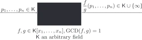
In [16] Kaltofen and Trager present a general method for evaluating separately the numerator and denominator of a rational function in n variables given by “black box” pro-cedure that evaluates the rational function at a point (see Figure1).

It is assumed that the black box procedure returns∞if

g(p1, . . . , pn) = 0. The separation algorithm computes the

∗

This material is based on work supported in part by the National Sci-ence Foundation under Grants Nos. CCR-0305314 and CCF-0514585.

Permission to make digital or hard copies of all or part of this work for personal or classroom use is granted without fee provided that copies are not made or distributed for profit or commercial advantage and that copies bear this notice and the full citation on the first page. To copy otherwise, to republish, to post on servers or to redistribute to lists, requires prior specific permission and/or a fee.

ISSAC’07, July 29–August 1, 2007, Waterloo, Ontario, Canada.

p1, . . . , pn∈K

−−−−−−−−−−−→

f, g∈K[x1, . . . , xn],GCD(f, g) = 1

Kan arbitrary field

f

g(p1, . . . , pn)∈K∪ {∞}

−−−−−−−−−−−−−−−−−−−→

Figure 1: Black box for rational function evaluation

values of f(p1, . . . , pn)/c ∈ K and g(p1, . . . , pn)/c ∈ Kfor

p1, . . . , pn in the coefficient field K, where c∈K\ {0}is a

fixed constant that selects the same associates of the numer-ator and denominnumer-ator polynomials for all evaluations. It is observed in [16] that the evaluation procedure can be com-bined with any sparse polynomial interpolation algorithm to compute the sparse representations off andg, namely

f /c=

tf

X

j=1 ψjx

dj,1 1 · · ·x

dj,n

n , g/c= tg

X

k=1 χkx

ek,1 1 · · ·x

ek,n

n ,

where ψj, χk ∈K\ {0}.Here we consider the sparse

poly-nomial interpolation algorithm in [13], which minimizes the number of polynomial evaluations using the early termina-tion paradigm. Our goal is to minimize the number of ratio-nal function evaluations in practice. Other work on sparse rational function interpolation is [8], which focuses on gen-eral decidability and complexity questions.

The combination of both the separation and the early ter-mination algorithms allows two major speedups. First, in [16] a homotopy is used so that the value off /c(p1, . . . , pn)

can be computed even wheng(p1, . . . , pn) = 0. However, the

algorithm in [13] can be performed for pointspτ

1, . . . , pτi−1, pκi,

pi+1, . . . , pn where pi (1 ≤i≤ n) that are uniformly

ran-domly selected from a sufficiently larger finite subsetS⊆K. We present the probabilistic analysis for a separation pro-cedure without a homotopy for such random points (see Lemma2.2). The change avoids the interpolation of a sec-ond variable. Secsec-ond, the sparse interpolation algorithm of [13] is executed simultaneously on f /c andg/c. Thus the early termination pruning techniques can be extended for obtaining numerator and denominator values: if a (partial) numerator or denominator polynomial is known to be com-plete, further polynomial values can be computed directly without rational recovery (see Section3).

(2)

deg(f) and ¯e≥deg(g) on page ). We have implemented our algorithm and demonstrate the performance on a selection of sparse rational functions (see Section5). An additional place for improvement arises when recovering numerator and denominator polynomials with integer coefficients, i.e., the case K = Q. The algorithm in [13] uses modular arith-metic (K = ZM, whereM is prime) and rational number

recovery [27,15]. It is possible to probabilistically recover the common denominator of the rational coefficients with-out individual numerator and denominator bounds [21], but thenM needs to be larger than is necessary with accurate bounds. Here we take advantage of the fact that several rational numbers are recovered simultaneously and employ the algorithm by [15] in a self-correcting manner, again with-out any individual numerator and denominator size bounds. Furthermore, we have implemented a rational vector recov-ery procedure based on Largarias’s [20] good simultaneous diophantine approximation algorithm. Via lattice basis re-duction, we can for certain inputs further reduce the size of the modulusM. We describe our two algorithms in Sec-tion4.

Finally, we investigate how numerical sparse interpola-tion algorithms [7] can be used together with our approach on numerical rational function black boxes, i.e., procedures that return the value of the rational function at a point as a floating point number that is an approximation of the ex-act value (contains “noise”). By making necessary changes in the procedure for separately evaluating the numerator and denominator, we are able to recover low degree sparse numerator and sparse denominator polynomials from ap-proximate values. We describe our apap-proximate algorithm and some remaining issues in Section6. Our approximate algorithm is related to numeric multivariate rational inter-polation (see, e.g., [1]). We note that our methods do not fit a set of given data points, which in the multivariate case leads to multiple solutions, but recovers a sparse rational function uniquely by evaluating at certain points.

2. EVALUATION OF THE NUMERATOR

AND DENOMINATOR

We first present an algorithm that returns the values at certain random points of fixed associates of the numerator and denominator polynomial for the black box of the ratio-nal functionf /g. The algorithm makes use of a univariate rational function recovery procedure, which we summarize for later reference in the following lemma [16, Lemma 1 on p. 315]

Lemma 2.1. Letd¯and¯ebe non-negative integers, and let

F(X), G(X), H(X)∈K[X], Kan arbitrary field,deg(H)<

¯

d+¯e+1,gcd(F, G) = 1; furthermore, letik,1≤k≤d¯+¯e+1,

be not necessarily distinct elements inKsuch that

F≡G H (mod (X−i1)· · ·(X−id¯+¯e+1)).

Defineh0(X) := (X−i1)· · ·(X−id¯+¯e+1),δ0 := ¯d+ ¯e+ 1,

andh1(X) :=H(X),δ1:= deg(H). Now lethl(X), ql(X)∈

K[X] be the l-th remainders and quotients respectively, in the Euclidean polynomial remainder sequence

hl−2(X)=ql(X)hl−1(X) +hl(X), δl:= deg(hl)< δl−1, l≥2.

In the exceptional caseH = 0the sequence is defined to be empty.

Finally, let wl(X), gl(X) ∈ K[X] be the multipliers in the

extended Euclidean schemewlh0+glh1=hl, namely,

w0:=g1:= 1, w1:=g0:= 0,

wl:=wl−2−qlwl−1, gl:=gl−2−qlgl−1 forl≥2.

Then there exists an indexj,1≤j, such thatδj≤d < δ¯ j−1.

For that index we have

hj≡gjH (mod (X−i1)· · ·(X−id¯+¯e+1))

and deg(gj)≤e.¯ ﬀ

(1)

Furthermore, if d¯≥ deg(F) and ¯e ≥deg(G) then F =

chj,G=cgj for somec∈K.

Our idea is similar to the one in [10, 16]. We obtain the values f(p1, . . . , pn)/c∈ K and g(p1, . . . , pn)/c∈ K at

p1, . . . , pn ∈ K by selecting once and for all random shift

valuesB2, . . . , Bn∈Kand by performing univariate rational

function recovery for

f(X, B2X−B2p1+p2, . . . , BnX−Bnp1+pn)

g(X, B2X−B2p1+p2, . . . , BnX−Bnp1+pn)

. (2)

Here the shift values Bi with high probability guarantee

that the leading coefficient of the denominatorg(X, B2X− B2p1+p2, . . . , BnX −Bnp1+pn), say, is independent of

the pi. By making that leading coefficient monic one then

can select the same associates for any pointp1, . . . , pn. The

values are computed by the evaluationX =p1. Aside from

our condition for the Bi, we also need to guarantee that

the fraction (2) cannot be reduced by a univariate polyno-mial GCD (and hence the denominator does not evaluate to 0). That we can enforce probabilistically by choosing the pointsp1, . . . , pnrandomly. The sparse polynomial

interpo-lation algorithm in [13], which we will deploy in Section3, re-quires the polynomial values atpτ

1, . . . , pτi−1, pκi, pi+1, . . . , pn

as well. Our next lemma shows that those also remain us-able with high probability.

Lemma 2.2. Letf, g∈K[x1, . . . , xn]withGCD(f, g) = 1,

let d = deg(f) and e = deg(g) and let t ≥ 1. Further-more, let B2, . . . , Bn ∈ K be such that λ1(B2, . . . , Bn) 6=

0 where λ1(β2, . . . , βn) is the leading coefficient in X of

g(X, β2X, . . . , βnX)∈(K[β2, . . . , βn])[X]. Finally, forJ≥

1andt≥1let

{(τj,1, . . . , τj,n)|1≤τj,k≤tfor all1≤j≤J,1≤k≤n},

(τ1,1, . . . , τ1,n) = (1, . . . ,1)

be a set ofJdistinct exponent vectors. Supposep1, . . . , pn∈

Sare chosen randomly and uniformly from a finite setS⊆K

of cardinality|S|. In addition, forj≥1let

f1, j(X) =f(X, B2X−B2p τj,1 1 +p

τj,2 2 , . . . , BnX−Bnp

τj,1 1 +p

τj,n

n ),

g1, j(X) =g(X, B2X−B2p τj,1 1 +p

τj,2 2 , . . . , BnX−Bnp

τj,1 1 +p

τj,n

n ). 9 > > =

> > ;

(3)

Then we have the following probability estimate:

Prob(GCD(f1, j(X), g1, j(X)) = 1for all1≤j≤J)

≥1−2((J−1)t+1) deg(f) deg(g) |S|

Proof: We first settle the case J = 1. For new variables

X,α1, . . . , αnwe define the map:

(3)

where

x17→X,

xi7→Bi(X−α1) +αi for all 2≤i≤n,

α17→α1.

Namely,

φ1(h(x1, x2, . . . , xn, α1))

=h(X, B2(X−α1) +α2, . . . , Bn(X−α1) +αn, α1).

The mapφ1 is a ring isomorphism by virtue of the inverse

map

φ−11 (X) =x1, φ−11 (α1) =α1,

φ−11 (αi) =xi−Bi(x1−α1) for all 2≤i≤n.

Namely,

φ−1₁ (h(X, α1, . . . , αn))

=h(x1, α1, x2−B2(x1−α1), . . . , xn−Bn(x1−α1)).

Next, we prove that GCD(φ1(f), φ1(g)) = 1. Suppose

GCD(φ1(f), φ1(g)) = ˆh1. Then we have φ1(f) = ˆf1ˆh1, φ1(g) = ˆg1hˆ1, for ˆf1, ˆg1, ˆh1 ∈ K[X, α1, . . . , αn]. We know

thatf=φ−1₁ ( ˆf1)φ−11 (ˆh1) andg=φ−11 (ˆg1)φ−11 (ˆh1). Now the

variableα1 vanishes in the polynomialsf andg. Therefore, α1also vanishes in the polynomialsφ−11 ( ˆf1), φ1−1(ˆg1), φ−11 (ˆh1),

i.e,φ−1_{( ˆ}_f

1), φ−1(ˆg1), φ−1(ˆh1)∈K[x1, . . . , xn]. Sincef and

g just have trivial GCD, we must have that φ−1₁ (ˆh1) ∈ K

and thus ˆh1∈K.

Now consider the Sylvester resultant

ρ1(α1, . . . , αn) = ResX(φ1(f), φ1(g))∈K[α1, . . . , αn].

Because GCD(φ1(f), φ1(g)) = 1, even in K[X, α1, . . . , αn],

we have ρ1 6= 0. Now suppose that for p1, . . . , pn ∈ K

we have ρ1(p1, . . . , pn) 6= 0. First, we have f1,1 6= 0 and g1,1 6= 0, wheref1,1 and g1,1 are defined in (3). We claim

that GCD(f1,1, g1,1) = 1. Here we need the condition on the Bi, since that condition guarantees that the leading

coeffi-cientλ1(B2, . . . , Bn) ofg1,1 is independent ofp1, . . . , pnand

therefore, considering the corresponding Sylvester matrices, we get

ResX(f1,1, g1,1) =± ρ1(p1, . . . , pn) λ1(B2, . . . , Bn)ν 6

= 0,

whereν= degX(φ1(f))−degX(f1,1), which establishes our

claim.

The probability estimate for t= 1 now follows from the Schwartz-Zippel lemma [28,24,3] and the degree estimate deg(ρ1)≤2 deg(f) deg(g).

Finally, we consider arbitraryJ. As before, forj≥1 and

h∈K[x1, x2, . . . , xn, α1] we introduce the map

φj(h(x1, x2, . . . , xn, α1)) =h(X, B2(X−α τj,1 1 ) +α

τj,2 2 , . . . , Bn(X−α

τj,1 1 ) +α

τj,n

n , α τj,1 1 ).

and the resultant

ρj(α1, . . . , αn) = ResX(φj(f), φj(g))∈K[α1, . . . , αn].

Now suppose that the leading coefficient inX of φ1(f) is σ∈K[α1, . . . , αn]\ {0}. Then the leading coefficient inX

of φj(f) is σ(α τj,1 1 , . . . , α

τj,n

n ), because the latter

polyno-mial remains non-zero. Thus degX(φj(f)) = degX(φ1(f)), ρj(α1, . . . , αn) =ρ1(α

τj,1 1 , . . . , α

τj,n

n )6= 0 and

ResX(f1, j, g1, j) =±ρj(p1, . . . , pn)/λ1(B2, . . . , Bn)µ

=±ρ1(p τj,1 1 , . . . , p

τj,n

n )/λ1(B2, . . . , Bn)µ,

whereµ= degX(φj(f))−degX(f1, j). Therefore, any point

p1, . . . , pn satisfies our lemma ifQJj=1ρ1(p τj,1 1 , . . . , p

τj,n

n )6=

0. The probability estimate follows from the degree estimate deg(ρ1(α

τj,1 1 , . . . , α

τj,n

n ))≤2tdeg(f) deg(g) forj≥2. 2

We can now state our evaluation algorithm, which includes a method for determining the degrees of the numerator and denominator polynomials.

Algorithm

Evaluation of Numerator and Denominator

Input: ◮ f(x1,x2,...,xn)

g(x₁,x₂,...,xn) ∈K(x1, x2, . . . , xn) input as a black

box (see above)

◮ _B

2, . . . , Bn: n−1 shift elements that are

ran-domly chosen from a sufficiently large finite set

S1⊆K ◮ _p

1, . . . , pn:nevaluation points that are randomly

chosen from a sufficiently large finite setS2⊆K ◮ _d,¯_¯_e_{: degree bounds ¯}_d_≥_deg(_f_{) and ¯}_e_≥_deg(_g₎ ◮ _{d, e} _{(optional): the degrees of}_f _and _g_,

respec-tively (with high probability)

◮ _τ

1, . . . , τn: a given exponent vector with 1≤τi≤

min( ¯d,e¯) Output: ◮ _{the value of}_f₍_pτ1

1 , . . . , pτnn)/candg(p τ₁

1 , . . . , pτnn)

/c(with high probability), wherecis the leading coefficient ofg(X, B2X, . . . , BnX)

(with high probability)

◮ _{or “failure,” in which case the random values}

input are diagnosed as unusable

The algorithm performs a Cauchy interpolation (rational function recovery) for

f1, j(X)/g1, j(X) mod (X−i1)· · ·(X−id+e+1),

where f1, j andg1, j are defined in (3) for (τj,1, . . . , τj,n) =

(τ1, . . . , τn) and il ∈ K are suitable values. After

mak-ing g1, j monic, the numerator and denominator values are

f1, j(pτ₁1) and g1, j(pτ₁1). From Lemma 2.2, we know that

GCD(f1, j, g1, j) = 1 inK[X] and therefore the Cauchy

in-terpolation algorithm recovers the proper images with high probability.

Casedeg(f) and deg(g) are given:

ev1 Compute (possibly in parallel)d+e+1 distinct elements

i1, . . . , id+e+1∈Kand

Al=

f

g(il, B2(il−p

τ₁ 1 )+p

τ₂

2 , . . . , Bn(il−pτ11)+p τn

n )6=∞

for all 1≤l≤d+e+1.

If deg(g1, j) = deg(g), i.e., the shift pointsB2, . . . , Bn

preserve the denominator degree, at most d+ 2e+ 1 elements inKneed to be tried since there are at most

eroots ofg1, j(X).

If more thanevalues inKyield∞when evaluating the rational function black box return with “failure.” Ei-ther the degrees are incorrect, or the projection points

B2, . . . , Bn and pτ₁1, . . . , pτnn are unlucky, or the black

(4)

ev2 By interpolation, compute a polynomialh1(X)∈K[X]

such that h1(il) = Al for all 1 ≤ l ≤ d+e+ 1 and

deg(h1)< d+e+ 1.

ev3 By the extended Euclidean algorithm in Lemma 2.1

compute ˆg,hˆsuch that

ˆ

h≡ghˆ 1 (mod (X−i1)· · ·(X−id+e+1)), deg(ˆh)≤d.

By construction we have deg(ˆg)≤e. If deg(ˆg)< ethen return “failure.”

If GCD(ˆg,ˆh) 6= 1 then return “failure.” In this case, there is no rational function for the computed points (see [6, Corollary 5.18]), so again the degrees are in-correct or the black box does not evaluate a rational function.

ev4 Return ˆh(pτ1

1 )/c and ˆg(p τ₁

1 )/c where c is the leading

coefficient of ˆg.

Cased¯≥deg(f) and ¯e≥deg(g) are given:

We determine the actual degrees by iterating onk=d+e+ 1 = 1,2, . . .In the previous case,eis used to terminate the search for valuesil on whichg1, j does not vanish. For this

we use the bound ¯einstead. The numerator degreedis used in Stepev3. Here we make the following change. First, we precompute for the threshold η ≥ 1 the rational function values

Um=

f

g(um, B2(um−p

τ₁ 1 ) +p

τ₂

2 , . . . , Bn(um−p₁τ1) +pτnn)6=∞

for all 1≤m≤η,

whereumare uniformly randomly chosen from a sufficiently

large finite subset S3 ⊆ K. Again, only η+ ¯e values are

tried before reporting “failure.” Then for each k we con-siderallremainder/co-factor pairs produced by the extended Euclidean algorithm, and which satisfy the degree bounds. A pair is accepted as f1, j/g1, j if it satisfies the input

de-gree bounds, co-primeness, and the corresponding fraction is equal toUmwhen evaluatingXatum, that for all 1≤m≤

η. In addition to returning the numerator and denominator values as in Step ev4, we also return their degrees. The interpolanth1 of Stepev2can be incrementally computed

fromk tok+ 1 using Newton interpolation (the method of divided differences). Note that the iteration is terminated in failure ifk >d¯+ ¯e, in which case the inputs are unlucky or wrong. 2

We have the following probabilistic analysis for our algo-rithm. Suppose the above algorithm is calledJ ≥1 times, using a single list of random shift elements B2, . . . , Bn, a

single pointp1, . . . , pnand the degreesd, ecomputed by the

first call with (τ1, . . . , τn) = (1, . . . ,1) and correct degree

bounds ¯d,¯e. Then the algorithm does not return “failure” and the returned values are equal the values off /candg/c

for allJ calls with probability no less than

“

1−deg(g) |S1|

”

bounds the probability thatλ1(B2, . . . , Bn)6=

0 (see Lemma2.2)

×“1−2((J−1)t+1) deg(f) deg(g) |S2|

”

bounds the probability

that all points are usable (Lemma2.2), conditional on the event that the shiftsBi work

×“1−θ2(d, e,d¯)

“θ₁(d, e,d,¯¯e)

|S3| ”η”

, where θ1 andθ2 are

de-fined below, bounds the probability that the correct degreesd, eare computed, conditional on good shifts and points. A wrong degree is returned if a false uni-variate continued fraction ˆh/gˆis accepted asf1,j/g1,j,

that is we have

(ˆhg1,j−f1,jgˆ)(um) = 0 for all 1≤m≤η. (4)

The largest degrees which need to be considered are deg(ˆh)≤min( ¯d, d+e) and deg(ˆg)≤min(¯e, d+e−1), the latter for the last falsek = d+e. Now the left polynomial in (4) has degree no more than

θ1(d, e,d,¯e¯) = max(min( ¯d, d+e)+e, d+min(¯e, d+e−1))

so all um accept one false ˆh/ˆg with probability no

more than (θ1(d, e,d,¯e¯)/|S3|)η. There are no more

thanθ2(d, e,d¯) =Pkd=1+e+1min(k,d¯+ 1) such fraction

candidates to be considered (for certain cases, one can lessen the bound using ¯e). The probability that at least one such event, namely acceptance of a false can-didate, occurs is then bounded from above by the sum of the probabilities for each event.

3. EARLY TERMINATION IN SPARSE

RA-TIONAL FUNCTION INTERPOLATION

We now describe the combination of the early termina-tion version [13] of Zippel’s [29] sparse multivariate interpo-lation algorithm with Algorithm Evaluation of Numerator and Denominator on page . Early termination is used to minimize the number of polynomial evaluations while keep-ing the size of the intermediate evaluation points small. Zippel’s algorithm reconstructs a sparse polynomial, h ∈ K[x1, . . . , xn] say, one variable at a time. A so-called

an-chor point p2, . . . , pn ∈ K is chosen. For i = 1,2, . . . , n

the univariate imagesψe₁,...,ei−1(xi, pi+1, . . . , pn)∈K[xi] of the coefficientsψe₁,...,ei−1(xi, . . . , xn)∈K[xi, . . . , xn] of the non-zero termsxe1

1 · · ·x ei−1

i−1 inh, viewed as a polynomial in x1, . . . , xi−1 with coefficient inK[xi, . . . , xn], are computed

by interpolation from valuesψe₁,...,ei−1(b

[κ]

i , pi+1, . . . , pn)∈

K, where b[iκ] ∈ Kforκ = 1,2, . . . Those values are found

from h(pτ

1, . . . , pτi−1, b[ κ]

i , pi+1, . . . , pn) for τ = 0,1, . . . by

solving a transposed Vandermonde system [2]. Zippel’s [28] ingenious observation is that for randompi any zero

coeffi-cient ofψe₁,...,ei−1(xi, pi+1, . . . , pn) is with high probability the value of a zero polynomial, thus reducing the size of the transposed Vandermonde system to the number of non-zero terms at stagei−1. D´ıaz and Kaltofen [4] introduce a ho-mogenizing variable x0 and interpolate ˜h(x0, x1, . . . , xn) =

h(x0x1, . . . , x0xn). Then it is known from their degrees in

x0 and x1, . . . , xi, respectively, that terms that do not

de-pend on xi+1, . . . , xn are complete and need not be

inter-polated any further (are “permanently pruned”). Kaltofen and Lee [13] perform the interpolation of eachψe₁,...,ei−1(xi,

pi+1, . . . , pn) by “racing” both the early termination version

of Newton interpolation and the early termination version of sparse univariate Ben-Or/Tiwari interpolation [14], that on the same evaluation points b[iκ] =p

κ

i. Then low degree

(5)

When combining the algorithm in [13] with Algorithm Evaluation of Numerator and Denominator on page we can take further advantage of temporary pruning and early ter-mination, namely when all terms of one of the numerator or denominator polynomials are completed (either temporarily or permanently). Because in that case, no univariate ratio-nal fraction recovery is needed for computing the values of the other remaining polynomial, and a single evaluation of the black box of the rational function suffices. We present a brief sketch of our algorithm.

Algorithm

Sparse Rational Function Interpolation Input: ◮ f(x1,x2,...,xn)

g(x₁,x₂,...,xn) ∈K(x1, x2, . . . , xn) input as a black

box

◮ ₍_x

1, . . . , xn): an ordered list of variables inf /g. ◮ _d,¯_e_¯_{: degree bounds ¯}_d_≥_deg(_f_{) and ¯}_e_≥_deg(_g₎

Output: ◮ _f₍_x

1, . . . , xn)/c and g(x1, . . . , xn)/c (with high

probability), wherec∈K.

◮ _{Or “failure”, in which case unlucky random}

el-ements have been selected (one can rerun the algorithm with new random values) or the black box does not evaluate a rational function of the given degree bounds.

et1 Sample shift elementsB2, . . . , Bnrandomly from a

suf-ficiently large finite setS1⊆K;

Initialize the anchor points: choose p0, p1, . . . , pn

ran-domly from a sufficiently large finite setS2⊆K;

Introduce the homogenizing variablex0 into f andg,

define ˜

f(x0, x1, . . . , xn)

˜

g(x0, x1, . . . , xn)

= f(x0x1, x0x2, . . . , x0xn)

g(x0x1, x0x2, . . . , x0xn)

.

et2 Interpolate Homogenizing Variablex0:

Inputting the shift elementsB2, . . . , Bnand ¯d,¯eto

Al-gorithm Evaluation of Numerator and Denominator on page , compute evaluations of ˜f and ˜g. The first such call returns degreesd, ethat with high probability are the degrees off and g. Note that for each evaluation one only needs deg(f) + deg(g) + 1 black box probes.

With the obtained values, interpolate the polynomials

f0 = ˜f(x0, p1, . . . , pn)/c and g0 = ˜g(x0, p1, . . . , pn)/c,

simultaneously using the racing algorithm described as above. Herecis the leading coefficient of the polyno-mialg(X, B2X, . . . , BnX).

If Algorithm Evaluation of Numerator and Denomina-tor on page or racing algorithm fail, then return “fail-ure”.

et3 Interpolate Next Variablexi:

Casef˜(x0, x1, . . . , xn)/c or ˜g(x0, x1, . . . , xn)/cis

com-pleted:

The values of the yet-to-be complete polynomial is com-puted directly by the black box and the completed poly-nomial in place of Algorithm Evaluation of Numerator and Denominator on page , and a stageisparse poly-nomial interpolation is performed as described above.

Casef˜(x0, x1, . . . , xn)/cand ˜g(x0, x1, . . . , xn)/care not

completed:

Interpolate fi = ˜f(x0, x1, . . . , xi, pi+1, . . . , pn)/c and

gi= ˜g(x0, x1, . . . , xi, pi+1, . . . , pn)/csimultaneously,

wh-ich is similar to Stepet2. As in the previous case, the numerator or denominator may be completed early.

et4 Recover f(x1, . . . , xn)/c and g(x1, . . . , xn)/c from fn

andgn, respectively. This step is non-trivial for certain

fields such as K = Q, when the scalar coefficients of both numerator and denominator can be reduced. See also Section4. 2

Note that our algorithm essentially performs simultaneous interpolation of two sparse polynomials, which are given by a black box that evaluates both at a given point. In our case, the black box operates differently when early termination has occurred, either temporarily or for the rest of the inter-polation task. One can naturally generalize our techniques to interpolating an entire vector of multivariate sparse poly-nomials and rational functions. In the latter case, additional savings are possible (see the end of Section4).

4. RATIONAL VECTOR RECOVERY

We now turn to the problem of recovering rational num-bers from their modular images. The constructive version [15, Theorem 5.1] of Axel Thue’s theorem establishes what is the corresponding integral property of the polynomials in Lemma2.1.

Theorem 4.1. Let a residue H ≥1, a modulusM, and boundsD, E≥2be integers such thatH < M,(D−1)(E−

1)< M < DE. Then the problem

F ≡GH (modM), |F|< D, F 6= 0, 0< G < E (5)

is solvable in integersF, Gif and only if∆ = GCD(H, M)< D. Furthermore, assuming that this is the case, let

U0 V0

=0 1,

U1 V1

, . . . ,UN VN

= H/∆

M/∆, VN≥

M

D−1 > E−1,

be the continued fraction approximations ofH/M and choose

l such that Vl < E ≤Vl+1. Then G1 = Vl, F1 =HVl−

M Ul is a solution for(5). The set of all solutions for (5)

exclusively either consists of λG1, λF1, where 1 ≤ λ <

min(E/G1, D/|F1|) or else consists of G1, F1 and G2, F2

with F1F2<0. In the latter case we can determineG2, F2

fromUl−1/Vl−1 orUl+1/Vl+1 inO((logM)2)binary steps.

Note thatD, E are bounds. In [15] examples for all three cases are given. If GCD(G, M) = 1 thenF/G≡H (modM) and a rational numberF/Gis recovered from its modulus. In modular arithmetic it is often known that such a solution exists. The exceptional case of two rational number candi-dates can be then resolved as in [27], by using a modulus

M so thatEis at least twice the denominator and selecting the solution with the smaller denominator as the recovered rational number, which is then F1/G1. If we choose the

modulus even larger, the last denominator Vl < E must

then be substantially smaller than E and a large quotient must occur. In [21] this observation is used to determine

l without E, assuming that the previous quotients in the continued fraction approximation are small.

We discuss simultaneous recovery Fi/G≡ Hi (modM)

for given H1, . . . , Ht ∈ZM. Again we wish to determinel

(6)

Algorithm

Rational Vector Recovery 1 Input: ◮ _M_≥_{2: a modulus;}_H

1, . . . , Ht∈ZM

◮ _s_{(optional): the range of small random residues;}

the number of random trials (optional) Output: ◮ _{G, D}_∈_Z≥2 _{that satisfy}

GCD(G, M) = 1,

(D−1)G < M < D(G+ 1),

|GHismodM|< Dfor all 1≤i≤t, 9 =

;

(6)

where smod denotes the absolutely smallest re-mainder (symmetric residue).

◮ _{or “failure,” in which case either the}

random-ization was unlucky or noG, D that satisfy (6) exist.

For a given number of trials, repeat the following recovery procedure. Then return “failure.”

vr1 Compute a random linear combination H ≡ γ1H1 +

· · ·+γtHt ∈ ZM where −s ≤ γi ≤ s are uniformly

randomly chosen. IfH= 0 go to next trial.

vr2 For each continued fractionUl/Vlwherel= 1,2, . . .of

H/M perform the tests in Stepsvr3andvr4

vr3 SetE ←Vl+ 1. If GCD(H, M)≥E go to next trial.

Compute the maximum bound D that satisfies (D−

1)(E−1)< M < DE. Set Gto G1 and possiblyG2

as computed by Theorem4.1. Note that for the second case in the proof of [15, Theorem 5.1], we currently assume the boundE. If GCD(G, M) >1 go to next value or trial.

vr4 Compute the maximum bound D that satisfies (D−

1)(E−1)< M < DE. If |GHismodM|< D for all

1≤i≤treturnG, D. Otherwise go to next trial. 2

Stepvr1is necessary becauseGis the least common mul-tiple of the individual rational denominators. Our formula-tion of the problem is different from [22]. And our algorithm produces the first of potentially multiple solutions to (6). Any solution, includingH1, . . . , Ht and H1 smod M, . . . , Ht smodM, i.e., G= 1 is a rational vector satisfying the

congruences for certain bounds. Note that the caseH1 =

· · ·=Htnaturally leads to multiple rational solutions. For

a given problem, a unique correct vector needs to be selected by other means. For the linear system problem [22], this can done by adjusting the boundDdownward.

In test trials, the Algorithm Rational Vector Recovery 1 above performs unexpectedly well. Provided M is suffi-ciently large to accommodate the numerator and denomina-tor sizes of the rational preimage and the size of the linear coefficientsγiof Stepvr1, the preimage is almost always

re-turned. This is because false denominators are removed in the self-correction testvr4. However, if the least common denominator is substantially larger than the denominators of the individual components, a number of trials is sometimes needed.

It is possible to replace the scalar continued fraction ap-proximation algorithm by a variant of the simultaneous dio-phantine approximation algorithm [20]. For a given vector

α= (A1/B1, . . . , At/Bt) and a given bound E one seeks a

denominatorGwith 1≤G≤Esuch that

max

1≤i≤t 

ρi|ρi= min ζi∈Z

˛ ˛ ˛ ˛

GAi Bi −

ζi ˛ ˛ ˛ ˛ ﬀ (7)

is minimized. Applying the minimization problem to α= (H1/M, . . . , Ht/M), one minimizes simultaneously |GHi−

ζiM|, i.e., the numerators Fi = ±M ρi with Fi ≡ GHi

(modM). In [20] an algorithm, which iteratively performs several lattice basis reductions, is described that for the minimum distance ρ[min]_E of (7) among any Gin the range 1≤G≤Ecomputes aG∗_with

1≤G∗≤√2t_·_E _and

max

1≤i≤t 

ρ∗i |ρ ∗ i = min

ζi∈Z

˛ ˛ ˛ ˛

G∗Hi M −ζi

˛ ˛ ˛ ˛ ﬀ

≤√5t2t−1_·_ρ[min] E .

One recovers F∗

i =±M ρ∗i ≡G∗Hi (modM). In order to

keeptsmall, one can use several random linear combinations of theHi instead of the entire vector.

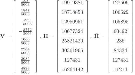
Example 4.2. Consider the rational vector V and two different modular imagesH=VmodM1 and ¯H=Vmod M2with moduliM1= 225 andM2= 217 given in Figure2.

V= 2 6 6 6 6 6 6 6 6 6 6 6 6 6 6 6 6 6 4 103 5003 1847 5003 −339 5003 −3772 5003 1060 5003 2234 5003 3085 5003 4826 5003 3 7 7 7 7 7 7 7 7 7 7 7 7 7 7 7 7 7 5

, H=

2 6 6 6 6 6 6 6 6 6 6 6 6 6 6 6 6 6 4 19919381 18718853 12950951 10677324 25821420 30361966 127431 16264142 3 7 7 7 7 7 7 7 7 7 7 7 7 7 7 7 7 7 5

, H¯ =

2 6 6 6 6 6 6 6 6 6 6 6 6 6 6 6 6 6 4 127509 106629 105895 60492 236 84334 127431 11214 3 7 7 7 7 7 7 7 7 7 7 7 7 7 7 7 7 7 5 .

Figure 2: Example vectors for rational recovery

Now we recover the vectorV from the two images using both algorithms:

Case 1 M1 = 225 = 33554432. Applying Algorithm

Ra-tional Vector Recovery 1 on page toH, we need for

s = 5 from 1 to 6 trials to recover V. Using the si-multaneous diophantine approximation algorithm with

E =⌈√M1⌉, we need a single lattice basis reduction

to recover the rational numbers vectorV.

Case 2 M2 = 217 = 131072. We fail to recover V using

Algorithm Rational Vector Recovery 1. However, we succeed to recoverVwithE =⌈√M2⌉after 5

itera-tions using our variant of the simultaneous diophantine approximation algorithm. 2

The problem of rational vector recovery of course applies also to our sparse rational function interpolation problem. Like in Algorithm Evaluation of Numerator and Denomina-tor on page and Algorithm Sparse Rational Function Inter-polation on page , for interpolatinga vectorof sparse ratio-nal functions with common denominator we can employ si-multaneous recovery of univariate fractionsFj/Gfrom their

modular imagesHjwith

Fj≡G Hj (mod (X−i1)· · ·(X−iκ)).

Olesh and Storjohann [22] show that for a number of points

(7)

a minimal polynomial basis algorithm. Thus the combined number of black box evaluations is reduced.

5. EXPERIMENTS

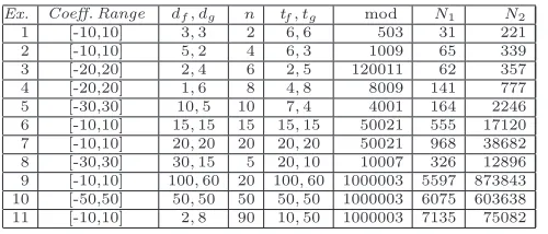
Algorithm Sparse Rational Function Interpolation on page has been implemented in Maple. We report the results of the experiments using our algorithm which are shown in Table1

below. For each example, we construct two relatively prime polynomials with random integer coefficients in the given range as the numerator and denominator. HereCoeff. Range is the range of the coefficients of the numerator and the de-nominator;df anddg are the degrees of the numerator and

the denominator of the rational function respectively;n de-notes the number of the variables of the rational function;tf

andtgare the number of the terms of the numerator and the

denominator respectively; mod is the integer of the modu-lus;N1denotes the number of the evaluations to interpolate

the rational function; N2 denotes the number of the black

box probes to interpolate the rational function. In all cases, for Algorithm Evaluation of Numerator and Denominator we use a threshold valueη= 3 in the first call.

Ex. Coeff. Range df, dg n tf, tg mod N1 N2 1 [-10,10] 3,3 2 6,6 503 31 221 2 [-10,10] 5,2 4 6,3 1009 65 339 3 [-20,20] 2,4 6 2,5 120011 62 357 4 [-20,20] 1,6 8 4,8 8009 141 777 5 [-30,30] 10,5 10 7,4 4001 164 2246 6 [-10,10] 15,15 15 15,15 50021 555 17120 7 [-10,10] 20,20 20 20,20 50021 968 38682 8 [-30,30] 30,15 5 20,10 10007 326 12896 9 [-10,10] 100,60 20 100,60 1000003 5597 873843 10 [-50,50] 50,50 50 50,50 1000003 6075 603638 11 [-10,10] 2,8 90 10,50 1000003 7135 75082

Table 1: Algorithm performance on benchmarks

6. SPARSE NUMERICAL INTERPOLATION

OF RATIONAL FUNCTIONS (SNIPR)

In [7] a numerical algorithm is given to interpolate the sparse multivariate polynomial from a multivariate approxi-mate black-box polynomial, making use of approxiapproxi-mate eval-uations at random primitive roots of unity. In order to in-terpolate the approximate sparse rational functions from the black box with noisy outputs, it is necessary to compute the numerator and denominator evaluations at a random prim-itive roots of unity.

In the exact case, the univariate rational function can be recovered by pad´e approximation. From Lemma2.1we know that the degree of the numerator and denominator can be determined by extended Euclidean schemes when the bound of the rational function is given. However, in the ap-proximate case, the polynomialHin Lemma2.1is not exact because of the approximate black box. So it is difficult to determine the degrees ofF and G, i.e. the degrees of the numerator and denominator. It is a remaining problem we have not completely addressed. For simplicity, we assume that the degree of rational function is known. In section 2, our exact algorithm performs a Cauchy interpolation for

f1, j(X)/g1, j(X) mod (x−i1)· · ·(x−id+e+1),

wheref1, j,g1, jare defined in (3). After makingg1, jmonic,

the numerator and denominator values aref1, j(pj₁), g1, j(pj₁).

Now we describe our method to compute the numerical evaluation of the numerator and denominator in detail. Ac-cording to our exact algorithm and the numerical algorithm for multivariate polynomial interpolation in [7], we choose the shift elements and variable values to be the roots of unity, namely Bj = exp(2sjπi/bj) ∈ C (i = √−1 and

2≤j≤n) andpk= exp(2sn+kπi/bn+k)∈C(1≤k ≤n)

where b2, . . . , b2n ∈ Z>0 are pairwise relatively prime such

that bl > max(d, e) (d, e the numerator and denominator

degrees) and whereslare random integers with 1≤sl< bl.

In order to recover the univariate polynomialsf1, j,g1, j, in

place of extended Euclidean schemes we apply to solve the Toeplitz-like linear system like Example on page 302 in [11]:

w(x)h0(X) +g1, j(X)h1(X)−f1, j(X) = 0 (8)

where h0(X) = (X−i1)· · ·(X−id+e+1),h1(X) is a

inter-polant such thath1(ik) =f1, j(ik)/g1, j(ik) for all 1≤k≤

d+e+ 1, and the degrees off1, j, g1, j are d, erespectively.

From the equation (8) we get a (2d+e+ 1)×(2d+e+ 2) matrix calledM. Since the row dimension ofM is one less than the column dimensionM. The system (8) always have a solution. f1, j,g1, jare obtained from the null space ofM.

Then we get the numerator and denominator values from

f1, j,g1, j.

In order to obtain a better solution, we can oversample at

d+e+ 1 +ζ points, whereζ ≥1, compute the polynomi-als h0(X) and h1(X), and then compute the approximate

solutionx of the overdetermined system: M·x ≈0. This problem is a structured total squares problem since the ma-trixAhas a Toeplitz-block structure (cf. [9]). We apply the Structured Total Least Norm (STLN)[23] method to obtain the approximate solution. As [19, 17] described,bcan be chosen a column ofM andA are formed by the remaining columns. We seek to compute the minimal structure pre-serving perturbation h, E such that (A+E)·x = b+h. Then we obtain the coefficients of univariate numerator and denominator fromx.

Example 6.1. Consider the rational functionf /g:

f=x3+y3+3x y+4x+1 and g= 3x3+2xy2+5xy+4x+5.

The noise for the black box off /gis in the range of 10−9≈

10−7_{. Choose}_p

1= exp(2πi/5), p2= exp(2πi/11) andB2=

exp(2πi_/_{13). We seek to compute the approximate}

evalua-tion of the numerator and denominator: f1, j(pj₁), g1, j(pj₁),

1 ≤j ≤9. We use STLN method to solve the overdeter-mined system and then obtain two lists of the values of the numerator and denominator Cj, Dj,1 ≤ j ≤ 9. Now we

check the backward error of our evaluation:

9 X

j=1

kCj−f(pj1)/ck2+kDj−g(pj1)/ck2= 3.45097×10−11

wherec= 4.13613 + 1.64597iis the leading coefficient of the polynomialg(X, B2X).

(8)

˜

f= (0.20872−0.08306i₎_y3_{+ (0}_.₂₀₈₇₂₋₀_.₀₈₃₀₅i₎_x3

+ (0.62616−0.24918i₎_{x y}_{+ 0}_.₈₃₄₈₇₋₀_.₃₃₂₂₄i₎_x

+ 0.20872−0.08306i_,

˜

g= (0.62616−0.24918i₎_x3_{+ (0}_.₄₁₇₄₄₋₀_.₁₆₆₁₂i₎_xy2

+ (1.04359−0.41529i₎_xy_{+ (0}_.₈₃₄₈₇₋₀_.₃₃₂₂₄i₎_x

+ 1.04356−0.41529i_.

The backward error iskf˜−f /ck2

2+kg˜−g/ck22= 5.08936×

10−14. 2

In the exact case, we require that the polynomialsf1, j and

g1, j are relatively prime. Now one approach is to check

whetherf1, jandg1, j have an approximate GCD. First, for

the given map and the input degrees of the rational function (d, e) we use our STLN method to computef1, j, g1, j from

(8), and compute the backward error:

error1=kw(X)h0(X) +g1, j(X)h1(X)−f1, j(X)k.

Then decreasing the input degrees as (d−1, e−1), we con-struct the overdetermined system from (8), where the de-grees of ˆf1, j,gˆ1, j are d−1, e−1 respectively. Then we

compute ˆf1, j and ˆg1, jand compute the backward error:

error2=kwˆ(X)h0(X) + ˆg1, j(X)h1(X)−fˆ1, j(X)k.

Suppose the ratio Υ =error2/error1 is sufficient large, that

is Υ> εwhereεis a chosen large value. We can declare that

f1, jandg1, jhave no approximate GCD, that isf1, j(pj1) and f1, j(pj1) are the approximate evaluationf(p

j

1, . . . pjn)/cand

f(pj₁, . . . pj

n)/c. Otherwise,f1, j and g1, j have a nearby

ap-proximate GCD. Then we start fresh and select newB2, . . . , Bn or new p1, . . . , pn to construct the new map.

There-fore, we need to find B2, . . . , Bn and p1, . . . , pn, and

com-pute f1, j, g1, j such that they are relatively prime for all

1 ≤j ≤J. In the exact case, from Lemma 2.2we know thatf1, j andg1, jare relatively prime with high probability

for all 1≤j≤J. In the approximate case it seems difficult to haveJ consecutive approximately relatively prime pairs

f1, j and g1, j. We have overcome those difficulties by

per-forming Zippel’s sparse interpolation method [29] directly on sparse rational functions with noisy values [18].

Acknowledgement: We thank Wen-shin Lee for providing her nu-meric sparse interpolation code to us, Arne Storjohann for sending us [22] and discussions on rational vector recovery, and Lihong Zhi for discussions on numerical univariate rational function recovery.

7. REFERENCES

[1] Becuwe, S., Cuyt, A., and Verdonk, B.Multivariate rational interpolation of scattered data. InLarge-Scale Scientific Computing(Heidelberg, Germany, 2004), I. Lirkov,

S. Margenov, J. Wasniewski, and Y. Plamen, Eds., vol. 2907 of

Lect. Notes Comput. Sci., Springer Verlag, pp. 204–213. [2] Ben-Or, M., and Tiwari, P.A deterministic algorithm for

sparse multivariate polynomial interpolation. InProc. Twentieth Annual ACM Symp. Theory Comput.(New York, N.Y., 1988), ACM Press, pp. 301–309.

[3] DeMillo, R. A., and Lipton, R. J.A probabilistic remark on algebraic program testing.Information Process. Letters 7, 4 (1978), 193–195.

[4] D´ıaz, A., and Kaltofen, E. FoxBoxa system for manipulating symbolic objects in black box representation. InProc. 1998 Internat. Symp. Symbolic Algebraic Comput. (ISSAC’98)

(New York, N. Y., 1998), O. Gloor, Ed., ACM Press, pp. 30–37. [5] Dumas, J.-G., Ed.ISSAC MMVI Proc. 2006 Internat. Symp.

Symbolic Algebraic Comput.(New York, N. Y., 2006), ACM Press.

[6] von zur Gathen, J., and Gerhard, J.Modern Computer Algebra. Cambridge University Press, Cambridge, New York, Melbourne, 1999. Second edition 2003.

[7] Giesbrecht, M., Labahn, G., and Lee, W.Symbolic-numeric sparse interpolation of multivariate polynomials. In Dumas [5], pp. 116–123.

[8] Grigoriev, D. Y., Karpinski, M., and Singer, M. F.

Computational complexity of sparse rational function interpolation.SIAM J. Comput. 23(1994), 1–11.

[9] Kai, H.Rational function approximation and its ill-conditioned property. In Wang and Zhi [26], pp. 47–53. Preliminary version in [25], pp. 62–64.

[10] Kaltofen, E.Greatest common divisors of polynomials given by straight-line programs.J. ACM 35, 1 (1988), 231–264. [11] Kaltofen, E.Asymptotically fast solution of Toeplitz-like

singular linear systems. InProc. 1994 Internat. Symp. Symbolic Algebraic Comput. (ISSAC’94)(New York, N. Y., 1994), ACM Press, pp. 297–304. Journal version in [12]. [12] Kaltofen, E.Analysis of Coppersmith’s block Wiedemann

algorithm for the parallel solution of sparse linear systems.

Math. Comput. 64, 210 (1995), 777–806.

[13] Kaltofen, E., and Lee, W.Early termination in sparse interpolation algorithms.J. Symbolic Comput. 36, 3–4 (2003), 365–400. Special issue Internat. Symp. Symbolic Algebraic Comput. (ISSAC 2002). Guest editors: M. Giusti & L. M. Pardo.

[14] Kaltofen, E., Lee, W.-s., and Lobo, A. A.Early termination in Ben-Or/Tiwari sparse interpolation and a hybrid of Zippel’s algorithm. InProc. 2000 Internat. Symp. Symbolic Algebraic Comput. (ISSAC’00)(New York, N. Y., 2000), C. Traverso, Ed., ACM Press, pp. 192–201.

[15] Kaltofen, E., and Rolletschek, H.Computing greatest common divisors and factorizations in quadratic number fields.

Math. Comput. 53, 188 (1989), 697–720.

[16] Kaltofen, E., and Trager, B.Computing with polynomials given by black boxes for their evaluations: Greatest common divisors, factorization, separation of numerators and denominators.J. Symbolic Comput. 9, 3 (1990), 301–320. [17] Kaltofen, E., Yang, Z., and Zhi, L.Approximate greatest

common divisors of several polynomials with linearly constrained coefficients and singular polynomials. In Dumas [5], pp. 169–176. Full version, 21 pages. Submitted, December 2006.

[18] Kaltofen, E., Yang, Z., and Zhi, L.On probabilistic analysis of randomization in hybrid symbolic-numeric algorithms. In

Proc. Internat. Workshop on Symbolic-Numeric Comput. 2007 (New York, N. Y., 2007), M. Moreno Maza, Ed., ACM Press. To appear.

[19] Kaltofen, E., Yang, Z., and Zhi, L.Structured low rank approximation of a Sylvester matrix. In Wang and Zhi [26], pp. 69–83. Preliminary version in [25], pp. 188–201.

[20] Lagarias, J. C.The computational complexity of simultaneous diophantine approximation problems.SIAM J. Comp. 14

(1985), 196–209.

[21] Monagan, M.Maximal quotient rational reconstruction: An almost optimal algorithm for rational reconstruction. In

ISSAC 2004 Proc. 2004 Internat. Symp. Symbolic Algebraic Comput.(New York, N. Y., 2004), J. Gutierrez, Ed., ACM Press, pp. 243–249.

[22] Olesh, Z., and Storjohann, A.The vector rational function reconstruction problem, Sept. 2006. Manuscript, 14 pages. [23] Park, H., Zhang, L., and Rosen, J. B.Low rank approximation

of a Hankel matrix by structured total least norm.BIT 39, 4 (1999), 757–779.

[24] Schwartz, J. T.Fast probabilistic algorithms for verification of polynomial identities.J. ACM 27 (1980), 701–717.

[25] Wang, D., and Zhi, L., Eds.Internat. Workshop on Symbolic-Numeric Comput. SNC 2005 Proc.(2005). Distributed at the Workshop in Xi’an, China, July 19–21. [26] Wang, D., and Zhi, L., Eds.Symbolic-Numeric Computation.

Trends in Mathematics. Birkh¨auser Verlag, Basel, Switzerland, 2007.

[27] Wang, P. S., Guy, M. J. T., and Davenport, J. H.P-adic reconstruction of rational numbers.SIGSAM Bulletin 16, 2 (May 1982), 2–3.

[28] Zippel, R.Probabilistic algorithms for sparse polynomials. In

Symbolic and Algebraic Computation (Heidelberg, Germany, 1979), vol. 72 ofLect. Notes Comput. Sci., Springer Verlag, pp. 216–226. Proc. EUROSAM ’79.

On exact and approximate interpolation of sparse rational functions