CopyrightÓ2009 by the Genetics Society of America DOI: 10.1534/genetics.108.099028
Multiple-Interval Mapping for Quantitative Trait Loci With a
Spike in the Trait Distribution
Wenyun Li* and Zehua Chen
†,1*School of Mathematics and Computational Science, Sun Yat-Sen University, Guangzhou, People’s Republic of China 510275 and †Department of Statistics and Applied Probability, National University of Singapore, Singapore 117546
Manuscript received November 24, 2008 Accepted for publication February 16, 2009
ABSTRACT
For phenotypic distributions where many individuals share a common value—such as survival time following a pathogenic infection—a spike occurs at that common value. This spike affects quantitative trait loci (QTL) mapping methodologies and causes standard approaches to perform suboptimally. In this article, we develop a multiple-interval mapping (MIM) procedure based on mixture generalized linear models (GLIMs). An extended Bayesian information criterion (EBIC) is used for model selection. To demonstrate its utility, this new approach is compared to single-QTL models that appropriately handle the phenotypic distribution. The method is applied to data from Listeria infection as well as data from simulation studies. Compared to the single-QTL model, the findings demonstrate that the MIM procedure greatly improves the efficiency in terms of positive selection rate and false discovery rate. The method developed has been implemented using functions in R and is freely available to download and use.
M
ANY statistical methods for mapping quantitative trait loci (QTL) have been developed for traits with regular distributions. These include single-interval mapping (Landerand Botstein1989), marker-basedregression (Cowen 1989; Moreno-Gonzalez 1992),
composite-interval mapping ( Jansen1993; Jansenand
Stam 1994; Zeng 1994), multiple-interval mapping
(Kao et al. 1999; Kao and Zeng 2002), and methods
especially for binary traits (see,e.g., Xuand Atchley
1996; Visscheret al.1996; Xuet al.1998; Yiand Xu2000;
McIntyreet al.2001).
Recently, Broman(2003) considered the traits with
distribution having a spike,i.e., a mixture of a regular distribution and a single-point mass. This type of trait is common in survival analysis and tumor studies (see,e.g., Boyartchuket al.2001; Hunteret al.2001). Broman
(2003) studied several single-QTL methods. The com-mon feature of these methods is that putative QTL are considered one at a time. The single-QTL methods can be efficient for identifying QTL-bearing chromosomes. But if they are used to identify individual QTL, there is a potential to commit a high false discovery rate due to the existence of spurious genotype correlations between loci not in linkage disequilibrium (LD) with QTL and those in LD with QTL.
A natural alternative to single-QTL methods is to con-sider multiple QTL simultaneously. In this article, we consider a multiple-interval mapping (MIM) procedure based on mixture generalized linear models (GLIM) for traits with the spike feature. An EM algorithm for the mixture GLIM and a forward procedure using an extended Bayesian information criterion (EBIC) (see Chenand Chen2008) are developed. The MIM
pro-cedure is illustrated with the Listeria data (Boyartchuk
et al.2001) that were analyzed by Broman(2003), using
the single-QTL methods mentioned above. Simulation studies are carried out to compare the MIM procedure with the single-QTL methods.
METHODS
For simplicity, we consider backcross designs without loss of generality. Let the marker genotypes of an interval be coded byxas follows:x¼1, if both markers are homozygous;x¼2, if the left one is homozygous and the right one is heterozygous; x¼3, if the left one is heterozygous and the right one is homozygous; andx¼ 4, if both markers are heterozygous. Letyibe the trait
value of individual i and xij be its genotype code on
interval j. Denote bydijthe unobservable genotype of
individualiat a putative QTL on intervalj, wheredij¼1,
if the genotype is homozygous, and 0 otherwise. The probability thatdij¼1 is determined byxijandrj, where
rjis the recombination fraction between the left marker
and the putative QTL of intervalj. Letp(rj,xij) denote
this probability.
Supporting information is available online athttp://www.genetics.org/ cgi/content/full/genetics.108.099028/DC2.
1Corresponding author:Department of Statistics and Applied Probability, National University of Singapore, 3 Science Dr. 2, Singapore 117546. E-mail: [email protected]
The multiple-QTL mixture GLIM: Consider anym intervals. Letdi ¼ ðdi1;. . .;dimÞ. Assume that the
condi-tional density function ofyigivendiis
½1pðdiÞ1zi½pðdiÞfðyi;diÞzi; ð1Þ
where zi ¼ I{yi 6¼ 0}, pðdiÞ ¼Pðzi ¼1Þ, and f is the
density function of an exponential family distribution. Then the joint density offðyi;diÞ;i¼1;. . .;ngis given
by
fðy;DÞ ¼Y n
i¼1
Ym
j¼1
pdijðrj;xijÞ½1pðrj;xijÞ1dij
3½1pðdiÞ1zi½pðdiÞfðyi;diÞzi; ð2Þ
where y¼ ðy1;. . .;ynÞ and D¼ ðd1;. . .;dnÞ. The
mar-ginal density ofyis obtained by summing up the second product over all possible values of thedij’s, which gives rise to a mixture of 2mcomponents of form (1).
Consider the general exponential family form of fðyi;diÞ,
fðyi;diÞ ¼exp
yiumðdiÞ bmðumðdiÞÞ
t 1Cðt;yiÞ
;
wheretis a dispersion parameter common to alli, andbm
is a monotone function related to the meanmðdiÞof the
distribution bymðdiÞ ¼ ð@bm=@umÞðumðdiÞÞ. Letg1(m(di))
be the link function that connectsmðdiÞ with a linear
predictor hmðdiÞ as hmðdiÞ ¼g1ðmðdiÞÞ. If only the
main effects of the QTL are considered, hmðdiÞ ¼
bm01 Pm
j¼1bmjdij. If epistasis effects among the
QTL are considered, hmðdiÞ ¼bm01 Pm
j¼1bmjdij1
P
1#j,k#mgmjkdijdik. Similarly, let pðdiÞ be related to a
linear predictorhp(di) through another link functiong2. The linear predictor hp has the same structure as hm.
For example, in the main-effect-only model,hpðdiÞ ¼
bp01 Pm
j¼1bpjdij. A common choice forg2is the logistic linkg2ðpÞ ¼logðp=ð1pÞÞ.
The mixture GLIM described above forms the basis of the MIM procedure. For details on GLIM, the reader is referred to McCullaghand Nelder(1989).
The EM algorithm: In the EM algorithm, the un-observable QTL genotypesDare treated as missing data. The pairðD;yÞis considered as the complete data andy
as the incomplete data. The parameters to be estimated arebm; bp, the coefficient vectors in the two linear
pre-dictors, andr, the vector of recombination fractions, as well ast, the dispersion parameter. The EM algorithm alternates iteratively between an E-step and an M-step. In an E-step, the conditional expectation of the log likeli-hood of the complete data,E½logfðy;DÞ jy;b0
m;b
0
p;r
0;t0,
is computed at the most updated values ofbm;bp;r;t. In
an M-step, the conditional expectation is maximized with respect to the parameters. Let upðdiÞ ¼lnðpðdi;bpÞ=
ð1pðdi;bpÞÞÞandbp(up)¼ln(11exp(up)). The log
density of the complete data, logfðy;DÞ, is expressed as follows:
Lðbm;bp;r;tÞ
¼X
n
i¼1
Xm
j¼1
½dijlnðpðrj;xijÞÞ1ð1dijÞlnð1pðrj;xijÞÞ
11
t Xn
i¼1
zi½yiumðdi;bmÞ bmðumðdi;bmÞÞ
1X
n
i¼1
ziupðdi;bpÞ bpðupðdi;bpÞÞ
½
¼L0ðrÞ1
1
tL1ðbmÞ1L2ðbpÞ:
Letðk1;. . .;kmÞbe anm-tuple withkj’s taking values 0
or 1. Define Dik1...km ¼
Qm
j¼1Ifdij¼kjg. Let umk1...km ¼
umððk1;. . .;kmÞ;bmÞ and upk1...km ¼upððk1;. . .;kmÞ;bpÞ.
ThenL1ðbmÞandL2ðbpÞcan be expressed as
L1ðbmÞ ¼ X
ðk1...kmÞ
½umk1...km
Xn
i¼1
ziyiDik1...kmbmðumk1...kmÞ
Xn
i¼1
ziDik1...km;
L2ðbpÞ ¼ X
ðk1...kmÞ
½upk1...km
Xn
i¼1
ziDik1...kmbpðupk1...kmÞ
Xn
i¼1 Dik1...km;
where the sums are taken over all possible m-tuples ðk1;. . .;kmÞ. The E-step thus is reduced to the
compu-tation of the conditional expeccompu-tationsEðDik1...kmjyÞ, and
the M-step is broken down into three separate maximi-zation problems. For ease of notation, in what follows, we use the same notation for Dik1...km, dij, and their
respective conditional expectations. Since L0ðrÞis the sum of m sums, each of them involving a different position parameter, the maximization ofL0ðrÞis further broken down into mmaximization problems. Each of them can be solved easily by a grid-point search pro-cedure. The maximization ofL1ðbmÞandL2ðbpÞcan be
carried out by two separate iterated weighted least-squares procedures that we describe as follows.
Letxk1...km be the row vector of the covariate values in
the linear predictors withd¼ ðk1;. . .; kmÞ. LetXbe the
matrix obtained by stacking the xk1...km’s one above
another in lexicographical order; i.e., the indexes ðk1;. . .;kmÞ are in the order (00. . .00), (00. . .01),
(00. . .10), ð00. . .11Þ;. . ., ð11. . .11Þ. Define WmðbmÞ
as the diagonal matrix with diagonal elementswmk1...km
given byD½kz
1...km=½g19ðmk1...kmÞ
2
b$mðumk1...kmÞ, wheremk1...km is
the mean value corresponding to d¼ ðk1;. . .;kmÞ,
D½kz
1...km ¼
Pn
i¼1ziDik1...km, g19 is the first derivative of g1,
and b$m is the second derivative of bm. Define
zmðbmÞ ¼Xbm1vmðbmÞ, where vmðbmÞ is the vector
with its (k1. . .km)th component given by
g91ðmk1...kmÞðD
½zy
k1...km=D
½z
k1...km mk1...kmÞ, where D
½zy
k1...km ¼
Pn
i¼1ziyiDik1...km. Similarly, define WpðbpÞ and zpðbpÞ
by replacingg1; bm; bm; D ½z
, and D[zy]withg
2;bp;bp,
D[1], and D[z], respectively, whereD½1
k1...km ¼
Pn
i¼1Dik1...km.
The M-step for updatingbmandbpis then realized by
iteratively solving the following equations:
X9WmðbOLDm ÞXbNEWm ¼X9WmðbOLDm ÞzmðbOLDm Þ;
X9WpðbOLDp ÞXbNEWp ¼X9WpðbOLDp ÞzpðbOLDp Þ:
After bm is updated, the dispersion parameter t is
updated by the average squared Pearson’s residuals associated with L1. The EM algorithm above is de-veloped along the same line as that in Chen and Liu
(2009).
Multiple-interval mapping procedure:The MIM pro-cedure makes use of a model selection criterion adapted from the EBIC recently developed by Chenand Chen
(2008). For a model with m intervals, the adapted criterion is given by
2 lnLðbˆm;bˆp;ˆr;ˆtÞ1nmlnn12 ln
M m
;1,n,3;
where Mis the total number of intervals under study. The numbernmis considered as the effective number of unknown parameters in the model. For a model withm intervals, there aremcomponents in each ofbm;bp, and
r. But bp does not play the same role as bm.
Further-more, only a portion of the data involve bm, and a
position parameter cannot be counted fully as a free parameter in terms of its effect on the likelihood. For example, most backcross progenies have flanking markers that are either both homozygous or both heterozygous. In this case, the position of a putative QTL has little effect on the likelihood. A definite effective number, which is in fact dependent on the data, is difficult to determine. Thenadjusts the effective number according to the data. The choice ofnshould be data dependent. In thediscussion, somead hocrules
and an outline of a data-driven approach to the choice ofnare provided.
We use EBIC as the model selection criterion because, as has been shown, it is consistent if the number of covariates under consideration is of the orderO(nk
) for anykwherenis the sample size, but the ordinary BIC fails to be consistent ifk . 0.5 (see Chenand Chen
2008).
The MIM procedure starts with models containing only one interval. The model with the minimum EBIC is compared with the null model with no QTL at all. If the minimum is smaller than the EBIC of the null model, the interval contained in the model is selected and the procedure continues; otherwise, it stops. At a general step, suppose m intervals have already been selected. Then all the models containing thesemintervals plus an additional one are assessed. The minimum EBIC of these models is compared with that of the previous model consisting ofmintervals. If the minimum is still smaller, the additional interval corresponding to the minimum EBIC is selected, and the procedure contin-ues; otherwise, it stops. In the above procedure, if an additional interval to be added is adjacent to any one already selected, it is skipped to avoid potential
colinearity that might cause nonconvergence of the EM algorithm. To summarize, the procedure sequentially adds intervals to a tentative model if the EBIC of the model decreases. The procedure stops when the EBIC begins to increase. The intervals contained in the final model are taken as QTL-bearing ones.
EXAMPLE
The Listeria data of Boyartchuk et al. (2001) are
reanalyzed to illustrate the MIM procedure. The data consist of the time to death following infection with Listeria monocytogenesof 116 F2mice from an intercross between the BALB/cByJ and C57BL/6ByJ strains and the mice’s genotypes at 133 markers on 20 chromo-somes. The result obtained is compared with that of the single-QTL two-part model method considered by Broman(2003).
The single-QTL two-part model method is imple-mented with threshold value of 4.93 for the LOD score. This threshold value is obtained by 10,000 permutation replicates. The intercross version of the MIM procedure is applied withn¼2.5 in EBIC. The exponential family distribution f in the GLIM is taken as the normal distribution.
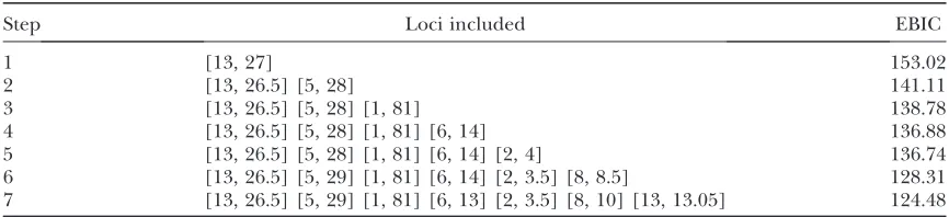
In the following, we use [k,d] to denote a locus on chromosomekwith a genetic distancedcM from the left end of that chromosome. The single-QTL two-part model method detects chromosomes 1, 5, and 13 as QTL-bearing ones. The loci at which the LOD score attains its maximum over each of the three chromo-somes are, respectively, [1, 81], [5, 30.9], and [13, 26.16]. The MIM procedure detects chromosome 1, 2, 5, 6, 8, and 13 as QTL-bearing ones. The detected loci in the last step of the MIM procedure are [1, 81], [2, 3.5], [5, 29.0], [6, 13.0], [8, 10.0], [13, 26.5], and [13, 13.05]. These results are summarized in Table 1. The loci and the EBIC value at each step of the MIM procedure are given in Table 2. The positions of the loci are slightly different from step to step because they are reestimated at each step. We cannot judge which result is better in this example. In the next section, we evaluate these two methods by simulation studies.
SIMULATIONS
The genetic map of the mouse genome in the exam-ple section is used to generate the data in simulation
studies; that is, the number and lengths of chromo-somes and the number and positions of markers on each chromosome are kept the same as those in the mouse genome. The genetic map is provided in sup-porting information,File S1.
Backcross progenies are generated according to the genetic map. In each replicate of the simulation, 5 chromosomes are randomly chosen from the first 19
chromosomes (the 20th chromosome is ignored since there are only two markers on it); on each of them, a QTL location is generated at random, and then the genotypes at these 5 QTL together with the 133 markers of 200 backcross progenies are generated. The trait values are generated under the assumption of no epistasis effect. Thebpis set at
bp¼ ð1:03;0:91;0:75;0:31;0:49;1:01Þ
and kept unchanged throughout. It is designed such that25% of the progenies will survive. Three settings ofbmare considered:
bm¼ ð4:650;1:605;1:065;0:585;0:855;1:410Þ;
bm¼ ð3:100;1:070;0:710;0:390;0:570;0:940Þ;
bm¼ ð1:550;0:535;0:355;0:195;0:285;0:470Þ:
The survival times are generated by a normal distribu-tion with mean equal tohmand variance 1. The threebm
-values correspond to the survival time heritabilities 0.63, 0.43, and 0.16, respectively.
The 95% threshold value for the LOD is simulated as 3.35 by 10,000 replicates and used in all three settings. The LOD scores are calculated at grid points spaced 1 cM apart. Three values ofn, 1.5, 2, and 2.5, are used in the EBIC. The MIM procedure and the single-QTL
two-part model method are applied to the same data. Their performances are assessed by positive selection rate (PSR) and false discovery rate (FDR). To make the comparison fair to the single-QTL two-part model method, we consider only whether or not a QTL-bearing chromosome is correctly identified, since sin-gle-QTL methods have been used mainly for this purpose. A chromosome is claimed as a QTL-bearing one if at least one of the selected loci falls in that chromosome. A claimed QTL-bearing chromosome is said to be a positive discovery if that chromosome does contain QTL. Otherwise, it is said to be a false discovery. The PSR and the FDR are defined as follows:
PSR¼ Number of positive discoveries
Total number of true QTL-bearing chromosomes;
FDR¼ Number of false discoveries
Total number of claimed QTL-bearing chromosomes:
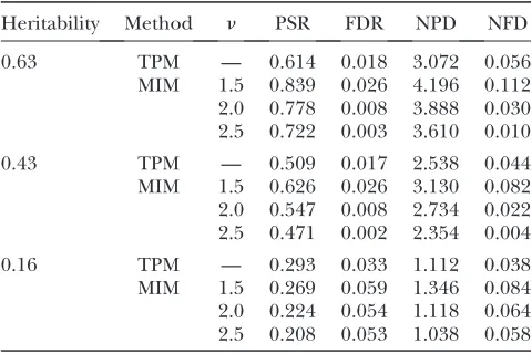
The simulation results over 500 replicates are given in Table 3. The findings are summarized as follows. With heritability 0.63, the MIM procedure has a much higher PSR with all the threen-values, a lower FDR whenn¼2 or 2.5, and a comparable FDR when n ¼ 1.5. With heritability 0.43, the MIM procedure has higher PSR and lower or comparable FDR whenn ¼2 or 1.5 and lower FDR and comparable PSR whenn¼2.5. We may claim that the MIM procedure is better than the single-QTL two-part model method when the heritability is moderate or high. However, in the case of heritability 0.16, the single-QTL two-part model method is better than the MIM procedure in terms of either PSR or FDR. An explanation is given below. The heritability consid-ered in the simulation accounts only for the nonsurvival portion and the QTL effect on the survival proportion is fixed. Any QTL with a heritability as low as 0.16 is hard to detect no matter what approach is used. The fairly sizeable PSR in this case is mainly due to the QTL effect on the survival proportion. In the EBIC criterion of the MIM procedure, an overpenalization arises when the effect on the survival time is in fact negligible. This explains why the PSR of the MIM procedure is lower in this case. A remedy for the problem of overpenalization is discussed in the next section.
TABLE 1
Loci (genetic distance in centimorgans from the left end of each chromosome) indicating evidence of
QTL detected by the single-QTL two-part model (TPM) and multiple interval-mapping
(MIM) in the example
Loci detected
Chromosome TPM MIM
1 81 81
2 — 3.5
5 30.90 29
6 — 13
8 — 10
13 26.16 13.05, 26.5
TABLE 2
The loci included and the corresponding EBIC value at each step of the MIM procedure in the example
Step Loci included EBIC
1 [13, 27] 153.02
2 [13, 26.5] [5, 28] 141.11
3 [13, 26.5] [5, 28] [1, 81] 138.78
4 [13, 26.5] [5, 28] [1, 81] [6, 14] 136.88
5 [13, 26.5] [5, 28] [1, 81] [6, 14] [2, 4] 136.74
6 [13, 26.5] [5, 29] [1, 81] [6, 14] [2, 3.5] [8, 8.5] 128.31
7 [13, 26.5] [5, 29] [1, 81] [6, 13] [2, 3.5] [8, 10] [13, 13.05] 124.48
DISCUSSION
We have demonstrated that the MIM procedure compares favorably with the single-QTL two-part model method when being used to identify QTL-bearing chromosomes. It has the further advantage of identify-ing individual QTL with accurately estimated positions. We discuss some further issues in this section.
In the MIM procedure considered in the previous sections, we do not distinguish between the QTL effects on the spike probability and on the survival time. This might lead to an overpenalization of the EBIC if only one type of effect exists and hence result in a reduced power for QTL detection. The procedure can be modified such that, when a new interval is considered, two substeps are taken, one for the effect on the spike probability and the other for the effect on the survival time. Correspondingly, the termnmlnnin the EBIC is replaced by nq ln n, where q counts the number of parameters of the model. When a new interval is considered, if only one type of effect is included, q increases by 1, and if both types of effect are included,q increases by 2.
In the simulation studies, we used differentn-values in EBIC. For smallern, the PSR is higher but the FDR is also higher, and vice versa. We give somead hocrules for the choice ofnhere. First, differentn-values should be used and the results compared. It is usually the case that, if the heritability is relatively high, the results will be similar in a range of n-values. If this is the case, the smallestnin this range produces the highest PSR and comparable FDR compared with other values in the range and should be used for a final decision. If there is a big discrepancy among different values, the choice
should be based on the purpose of the study. If the study is for confirmation, the FDR is a more serious concern, and a larger n should be taken. If the study is a preliminary step to detect regions for further investiga-tion, a smallernshould be taken.
A data-driven approach based on the idea of model averaging and bootstrapping can be used. The ap-proach is outlined as follows. Starting with a moderate n-value, a set of claimed QTL together with their estimated effects is obtained. Then the following bootstrap-like procedure is carried out. A random number, saym*, is generated from a Poison distribution with the mean as the number of claimed QTL. Thenm* loci, each on a different interval, are randomly selected from the genetic map and assigned as QTL, the effects of the QTL are generated using the estimated effects of the claimed QTL, and the trait values of individuals are generated by using the GLIM. Finally, the MIM pro-cedure with different n-values is applied to the gener-ated data, and the positive discoveries and false discoveries are obtained by comparing the claimed QTL with the assigned QTL. This process is repeated for a large number of times. The numbers of positive discoveries and false discoveries are averaged to provide estimates for PSR and FDR for each of the n-values. Then with the estimated PSR and FDR, the user can make a choice on the basis of a balanced consideration of PSR and FDR. A full development of the data-driven approach in more general settings is underway, which is beyond the scope of this article. We will report the general data-driven approach elsewhere.
The MIM procedure has been implemented using functions in the R package migtlm. The package will be updated soon to include a general function for the MIM procedure. The package can be downloaded from www.stat.nus.edu.sg/stachenz.
LITERATURE CITED
Boyartchuk, V. L., K. W. Broman, R. E. Mosher, S. F. F. D’Orazio, M. N. Starnbachet al., 2001 Multigenetic control ofListeria monocytogenessusceptibility in mice. Nat. Genet.27:259–260. Broman, K. W., 2003 Quantitative trait locus mapping in the case
of a spike in the phenotype distribution. Genetics163:1169– 1175.
Chen, J., and Z. Chen, 2008 Extended Bayesian information criteria for model selection with large model spaces. Biometrika95:759– 771.
Chen, Z., and J. Liu, 2009 Mixture generalized linear models for multiple interval mapping of quantitative trait loci in experimen-tal crosses. Biometrics (in press).
Cowen, N. M., 1989 Multiple linear regression analysis of RELP data sets used in mapping QTLs, pp. 113–116 inDevelopment and Ap-plication of Molecular Markers to Problems in Plant Genetics, edited by T. Helentjarisand B. Burr. Cold Spring Harbor Laboratory Press, Cold Spring Harbor, NY.
Hunter, K.W., K. W. Broman, T. LeVoyer, L. Lukes, D. Gozmaet al., 2001 Predisposition to efficient mammary tumor metastatic progression is linked to the breast cancer metastasis suppressor geneBrms1.Cancer Res.61:8866–8872.
Jansen, R. C., 1993 Interval mapping of multiple quantitative trait loci. Genetics135:205–211.
TABLE 3
The average positive selection rate (PSR), false discovery rate (FDR), number of positive discoveries (NPD),
and number of false discoveries (NFD) of the two approaches: the single-QTL two-part
model (TPM) and the multiple-interval mapping (MIM), over 500 replicates
in the simulation study
Heritability Method n PSR FDR NPD NFD
0.63 TPM — 0.614 0.018 3.072 0.056
MIM 1.5 0.839 0.026 4.196 0.112 2.0 0.778 0.008 3.888 0.030 2.5 0.722 0.003 3.610 0.010
0.43 TPM — 0.509 0.017 2.538 0.044
MIM 1.5 0.626 0.026 3.130 0.082 2.0 0.547 0.008 2.734 0.022 2.5 0.471 0.002 2.354 0.004
0.16 TPM — 0.293 0.033 1.112 0.038
MIM 1.5 0.269 0.059 1.346 0.084 2.0 0.224 0.054 1.118 0.064 2.5 0.208 0.053 1.038 0.058
Jansen, R. C., and P. Stam, 1994 High resolution of quantitative traits into multiple loci via interval mapping. Genetics 136: 1447–1455.
Kao, C. H., and Z. B. Zeng, 2002 Modeling epistasis of quantitative trait loci using Cockerham’s model. Genetics160:1243–1261. Kao, C. H., Z. B. Zengand R. D. Teasdale, 1999 Multiple interval
mapping for quantitative trait loci. Genetics152:1203–1216. Lander, E. S., and D. Botstein, 1989 Mapping Mendelian factors
underlying quantitative traits using RFLP linkage maps. Genetics 121:185–199.
McCullagh, P., and J. A. Nelder, 1989 Generalized Linear Models, Ed. 2. Chapman & Hall, London/New York.
McIntyre, L. M., C. Coffmanand R. W. Doerge, 2001 Detection and location of a single binary trait locus in experimental popu-lations. Genet. Res.78:79–92.
Moreno-Gonzalez, J., 1992 Genetic models to estimate additive and non-additive effects of marker-associated QTL using multi-ple regression techniques. Theor. Appl. Genet.85:435–444.
Visscher, P. M., C. S. Haleyand S. A. Knott, 1996 Mapping QTLs for binary traits in backcross and F-2 populations. Genet. Res.68: 55–63.
Xu, S., and W. R. Atchley, 1996 Mapping quantitative trait loci for complex binary diseases using line crosses. Genetics143:1417– 1424.
Xu, S., N. Yonash, R. L. Vallejoand H. H. Cheng, 1998 Mapping quantitative trait loci for complex binary traits using a heteroge-neous residual variance model: an application to Marek’s disease susceptibility in chickens. Genetica104:171–178.
Yi, N., and S. Xu, 2000 Bayesian mapping of quantitative trait loci for complex binary traits. Genetics155:1391–1403.
Zeng, Z. B., 1994 Precision mapping of quantitative trait loci. Genetics136:1457–1468.
Communicating editor: K. W. Broman
Supporting Information
http://www.genetics.org/cgi/content/full/genetics.108.099028/DC2
Multiple-Interval Mapping for Quantitative Trait Loci With a Spike in the
Trait Distribution
Wenyun Li and Zehua Chen
Li and Chen 2 SI
FILE S1
Multiple Interval Mapping for Quantitative Trait Loci with a Spike in the Trait Distribution
Wenyun Li and Zehua Chen
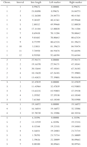
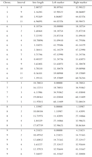
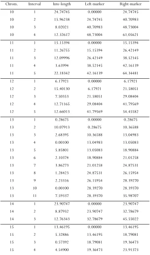
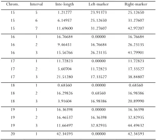
In this supporting information, we provide the genetic map used in the simulation studies of the paper. It is the genetic map of a mouse genome extracted from the Listeria data of BOYARTCHUK et al. (2001). The map contains 132 markers on 20 chromosomes. On each
Li and Chen 3 SI
TABLE S1
The genetic map of the mouse genome in the Listeria data
Chrom. Interval Inte-length Left-marker Right-marker 1 1 0.99675 0.00000 0.99675
1 2 23.85098 0.99675 24.84773
1 3 15.56588 24.84773 40.41361
1 4 9.58107 40.41361 49.99468
1 5 2.80552 49.99468 52.80020
1 6 17.31184 52.80020 70.11204
1 7 0.69438 70.11204 70.80642
1 8 9.81682 70.80642 80.62324
1 9 0.77299 80.62324 81.39623
1 10 3.53851 81.39623 84.93474 1 11 7.74920 84.93474 92.68394 1 12 0.95950 92.68394 93.64344
2 1 27.94171 0.00000 27.94171
2 2 19.16370 27.94171 47.10541
2 3 20.15644 47.10541 67.26185
2 4 10.13620 67.26185 77.39805
2 5 13.45825 77.39805 90.85630
3 1 32.47839 0.00000 32.47839
3 2 11.45964 32.47839 43.93803
3 3 13.65535 43.93803 57.59338
3 4 5.59202 57.59338 63.18540
3 5 7.65360 63.18540 70.83900
4 1 19.16072 0.00000 19.16072
4 2 16.16014 19.16072 35.32086
4 3 32.78230 35.32086 68.10316
5 1 6.10396 0.00000 6.10396
5 2 13.11939 6.10396 19.22335
5 3 0.32548 19.22335 19.54883
5 4 4.16831 19.54883 23.71714
5 5 1.78295 23.71714 25.50009
5 6 5.39656 25.50009 30.89665
5 7 0.00100 30.89665 30.89765
Li and Chen 4 SI
TABLE S2
The genetic map of the mouse genome in the Listeria data (Cont.)
Chrom. Interval Inte-length Left-marker Right-marker
5 8 2.00757 30.89765 32.90522
5 9 5.16285 32.90522 38.06807
5 10 5.95569 8.06807 44.02376 5 11 6.96095 44.02376 50.98471
6 1 8.18754 10.00000 18.18754
6 2 5.68464 18.18754 23.87218
6 3 7.22192 23.87218 31.09410
6 4 10.70096 31.09410 41.79506
6 5 3.35073 41.79506 45.14579
6 6 2.38411 45.14579 47.52990
6 7 3.71746 47.52990 51.24736
6 8 0.40337 51.24736 51.65073
6 9 3.65405 51.65073 55.30478
6 10 3.70510 55.30478 59.00988 6 11 0.36101 59.00988 59.37089 6 12 1.39155 59.37089 60.76244
7 1 18.78851 0.00000 18.78851
7 2 16.12211 18.78851 34.91062
7 3 6.11986 34.91062 41.03048
7 4 19.08361 41.03048 60.11409
7 5 11.97015 60.11409 72.08424
8 1 1.33987 0.00000 1.33987
8 2 10.08104 1.33987 11.42091
8 3 15.71975 11.42091 27.14066
8 4 5.84559 27.14066 32.98625
8 5 17.87739 32.98625 50.86364
9 1 4.21823 0.00000 4.21823
9 2 10.49742 4.21823 14.71565
9 3 12.60852 14.71565 27.32417
9 4 5.63227 27.32417 32.95644
9 5 12.37923 32.95644 45.33567
9 6 7.16837 45.33567 52.50404
Li and Chen 5 SI
TABLE S3
The genetic map of the mouse genome in the Listeria data (Cont.)
Chrom. Interval Inte-length Left-marker Right-marker 10 1 24.74745 0.00000 24.74745
10 2 15.96238 24.74745 40.70983
10 3 8.02021 40.70983 48.73004
10 4 12.32617 48.73004 61.05621
11 1 15.15394 0.00000 15.15394
11 2 11.26755 15.15394 26.42149
11 3 12.09996 26.42149 38.52145
11 4 3.63994 38.52145 42.16139
11 5 22.18342 42.16139 64.34481
12 1 6.17921 0.00000 6.17921 12 2 15.40130 6.17921 21.58051 12 3 7.50353 21.58051 29.08404
12 4 12.71165 29.08404 41.79569
12 5 12.66013 41.79569 54.45582
13 1 0.28675 0.00000 0.28675 13 2 10.07913 0.28675 10.36588 13 3 2.68395 10.36588 13.04983 13 4 0.00100 13.04983 13.05083 13 5 5.85801 13.05083 18.90884 13 6 2.10374 18.90884 21.01258 13 7 3.86273 21.01258 24.87531 13 8 1.28423 24.87531 26.15954 13 9 2.23316 26.15954 28.39270 13 10 0.00100 28.39270 28.39370 13 11 7.59337 28.39370 35.98707 14 1 23.90747 0.00000 23.90747 14 2 8.87932 23.90747 32.78679
14 3 12.76343 32.78679 45.55022
15 1 13.46195 0.00000 13.46195 15 2 5.32886 13.46195 18.79081 15 3 0.57392 18.79081 19.36473 15 4 4.54900 19.36473 23.91373
Li and Chen 6 SI
TABLE S4
The genetic map of the mouse genome in the Listeria data (Cont.)
Chrom. Interval Inte-length Left-marker Right-marker 15 5 1.21277 23.91373 25.12650 15 6 6.14957 25.12650 31.27607
15 7 11.69600 31.27607 42.97207
16 1 16.76684 0.00000 16.76684 16 2 9.46451 16.76684 26.23135
16 3 15.56766 26.23135 41.79901
17 1 11.72823 0.00000 11.72823 17 2 5.60704 11.72823 17.33527
17 3 21.51280 17.33527 38.84807
18 1 0.68560 0.00000 0.68560 18 2 16.29826 0.68560 16.98386 18 3 3.91604 16.98386 20.89990 19 1 16.36398 0.00000 16.36398
19 2 16.46537 16.36398 32.82935
19 3 11.66497 32.82935 44.49432